Stability of Periodic Soliton Equations under Short Range Perturbations

Abstract

We consider the stability of (quasi-)periodic solutions of soliton equations under short range perturbations and give a complete description of the related long time asymptotics.

So far, it is generally believed that a perturbed periodic integrable system splits asymptotically into a number of solitons plus a decaying radiation part, a situation similar to that observed for perturbations of the constant solution. We show here that this is not the case; instead the radiation part does not decay, but manifests itself asymptotically as a modulation of the periodic solution which undergoes a continuous phase transition in the isospectral class of the periodic background solution.

We provide an explicit formula for this modulated solution in terms of Abelian integrals on the underlying hyperelliptic Riemann surface and provide numerical evidence for its validity. We use the Toda lattice as a model but the same methods and ideas are applicable to all soliton equations in one space dimension (e.g. the Korteweg-de Vries equation).

I Introduction

One of the most important defining properties of solitons is their stability under perturbations. The classical result going back to Zabusky and Kruskal zakr states that a ”short range” perturbation of the constant solution of a soliton equation eventually splits into a number of stable solitons and a decaying background radiation component km . So the solitons constitute the stable part of arbitrary short range initial conditions. It is generally believed, and is claimed in kumi , that this remains valid when the constant background solution is replaced by a quasi-periodic one. Our aim here is to show this is not the case, and that a thus far undiscovered phenomenon appears in the description of the long time asymptotics.

Solitons on a (quasi-)periodic background have a long tradition and are used to model localized excitements on a phonon, lattice, or magnetic field background. Consequently, periodic solutions, as well as solitons travelling on a periodic background, are well understood. The first results were given over thirty years ago in the pioneering work by Kuznetsov and Mikhaĭlov kumi , where the stability of solitons of the Korteweg-de Vries equation on the background of the two-gap Weierstrass solution is investigated. There the $N$-soliton solution on this background is computed and it is shown that each soliton produces a phase shift. In addition, it is claimed that the asymptotic state of any short range initial condition is a set of solitons.

However, we will show that the asymptotic state is more complicated. The reason for this is related to the fact that the phase shifts of the solitons do not necessarily add up to zero. Hence there must be an additional feature making up for the overall phase shift. One might conjecture that solitons alone suffice to describe the asymptotic state at least in the case where the phase shifts add up to zero — which is the situation assumed in kumi . However, we will show that even if no solitons are present, the asymptotic state is not just the periodic background.

Due to the lack of powerful asymptotic analysis tools and computer power at the time of kumi it was impossible to identify this contribution then. However, it seems that this omission was neither pointed out in the literature nor was a complete description of the asymptotic state known.

To illustrate these facts, let us consider the doubly infinite Toda lattice in Flaschka’s variables (see e.g. tjac or ta )

$$\dot{b}(n,t) =2(a(n,t)^{2}-a(n-1,t)^{2}),$$

$$\dot{a}(n,t) =a(n,t)(b(n+1,t)-b(n,t)),$$

$(n,t)\in{\mathbb{Z}}\times{\mathbb{R}}$, where the dot denotes differentiation with respect to time. We will consider a quasi-periodic algebro-geometric background solution $(a_{q},b_{q})$ (e.g., any periodic solution) plus a short range (in the sense of emt2 ) perturbation $(a,b)$. The perturbed solution can be computed via the inverse scattering transform. The case where $(a_{q},b_{q})$ is constant is classical (see again tjac or ta ), but the more general case applicable here has only recently been analyzed in emt2 (see also emt ).

In Figures 1 the numerically computed solution corresponding to the initial condition $a(n,0)=1$, $b(n,0)=(-1)^{n}+2\delta_{0,n}$ is shown.

Figure 1: Numerically computed solution of the Toda lattice, with initial condition a period two solution perturbed at one point in the middle.

In each of these two pictures the two observed lines express the variables $a(n,t)$ at two frozen times $t=90$ and $t=165$. In areas where the lines seem to be continuous this is due to the fact that we have plotted a huge number of particles (around $1000$) and also due to the $2$-periodicity in space. So one can think of the two lines as the even- and odd-numbered particles of the lattice. We first note the single perturbation which separates two regions of apparent periodicity on the left. Comparing the two pictures we note that this is a solitary wave travelling to the left. Our computations show that it is indeed a soliton. To the right of the soliton, we observe three different areas of apparent periodicity (with period two). Between these areas there are transitional regions which interpolate between the different period two regions.

It is the purpose of this paper to give a complete explanation of this picture. We provide the details in case of the Toda lattice though it is clear that our arguments apply to other soliton equations as well.

II Quasiperiodic solutions in terms of Riemann theta functions

We begin by recalling that quasi-periodic solutions are most conveniently written in terms of Riemann theta functions (dub ). Such explicit formulae were first derived in the mid-70s thanks to the pioneering work of the Soviet school (Novikov, Its, Matveev, etc.). In the particular case of the Toda lattice the underlying Riemann surface is associated with the square root

$$R_{2g+2}^{1/2}(z)=-\prod_{j=0}^{2g+1}\sqrt{z-E_{j}},$$

where the numbers $E_{j}\in{\mathbb{R}}$ are the band edges of the spectrum $\Sigma=\bigcup_{j=0}^{g}[E_{2j},E_{2j+1}]$ of the corresponding Jacobi operator (see tjac ). We can picture this surface as the end result of cutting and pasting; we consider two ”sheets” (copies of the complex plane), we cut them along the segments $[E_{0},E_{1}]$, $[E_{2},E_{3}]$, … and paste the top side of the upper sheet to the bottom side of the lower sheet and the bottom side of the upper sheet to the top side of the lower sheet across every such segment.

On this Riemann surface we have a standard basis of normalized holomorphic differentials

$$\zeta_{j}=\frac{\sum_{k}c_{j}(k)z^{k}}{R_{2g+2}^{1/2}(z)}dz,\quad 1\leq j\leq g$$

(the constants $c_{j}(k)$ have to be determined from the usual normalization with respect to a canonical homology basis).

Introduce the vector

$$z_{j}(n,t) =\int_{E_{0}}^{\infty_{+}}\zeta_{j}-\sum_{k=1}^{g}\int_{E_{0}}^{\mu_{k}}\zeta_{j}$$

$$-n\int_{\infty_{-}}^{\infty_{+}}\zeta_{j}+t2c_{j}(g)-\underline{\Xi}_{E_{0}}\in{\mathbb{C}}^{g}.$$

Here $\infty_{\pm}$ are the points above $\infty$ on the upper/lower sheet and $\underline{\Xi}_{E_{0}}$ is the vector of Riemann constants. The numbers $\mu_{j}$ are some arbitrary points whose images in the complex plane lie in the $j$-th interior spectral gap. All possible choices form the isospectral class of quasi-periodic Jacobi operators with the given spectral bands. This isospectral class is just a $g$ dimensional torus, since the preimage of each gap with respect to the map that maps the surface to the complex plane (seen as one of the two sheets) consists of two parts, one on the upper and one the lower sheet, which form a circle.

Then the well-known formulas for the solutions read

$$a(n,t)^{2} =\tilde{a}^{2}\frac{\theta(\underline{z}(n+1,t))\theta(\underline{z}(n-1,t))}{\theta(\underline{z}(n,t))^{2}},$$

$$b(n,t) =\tilde{b}+\frac{1}{2}\frac{d}{dt}\ln\left(\frac{\theta(\underline{z}(n,t))}{\theta(\underline{z}(n-1,t))}\right),$$

where $\tilde{a}$, $\tilde{b}$ are the averages and

$$\theta(\underline{z})=\sum_{\underline{m}\in{\mathbb{Z}}^{g}}\exp 2\pi\mathrm{i}\left(\langle\underline{m},\underline{z}\rangle+\frac{\langle\underline{m},\underline{\tau}\,\underline{m}\rangle}{2}\right),\quad\underline{z}\in{\mathbb{C}}^{g},$$

is the Riemann theta function of our surface. The matrix $\tau$ is the matrix of $b$-periods of the normalized basis of holomorphic differentials $\zeta_{j}$.

III The main result

We will assume for simplicity that no solitons are present. In other words, we assume that the Jacobi operator above has no eigenvalues. The assumption is not crucial, since the solitons can be easily incorporated using a Darboux transform.

To obtain the long time asymptotics one reformulates the problem as a Riemann-Hilbert problem (RHP) on the underlying Riemann surface. This shows that the solution can be read off from the two by two matrix valued function $m$ that is meromorphic off the preimage of the spectrum $\Sigma$, with divisor satisfying

$$(m_{j1})\geq-\sum_{k}\mathcal{D}_{\mu_{k}^{*}(n,t)},\quad(m_{j2})\geq-\sum_{k}\mathcal{D}_{\mu_{k}(n,t)},$$

$j=1,2$, jump matrix given by

$$J(p,n,t)=\begin{pmatrix}1-|R(p,n,t)|^{2}&-\overline{R(p,n,t)}\\ R(p,n,t)&1\end{pmatrix},$$

$p\in\Sigma$, and normalization

$$m(p,n,t)\to\mathbb{I},\quad\text{as }p\to\infty_{+}.$$

This is similar to the RHP applicable to the constant background case, with the main difference being that we allow poles at the points $\mu_{j}(n,t)$, and their flip images $\mu_{j}^{*}(n,t)$ on the other sheet. The $g$ points $\mu_{j}(n,t)$ are uniquely defined by the Jacobi inversion problem

$$\sum_{k=1}^{g}\int_{E_{0}}^{\mu_{k}(n,t)}\zeta_{j}=\sum_{k=1}^{g}\int_{E_{0}}^{\mu_{k}}\zeta_{j}\\ +n\int_{\infty_{-}}^{\infty_{+}}\zeta_{j}-t2c_{j}(g).$$

This is a crucial point and related to the fact that our RHP is no longer formulated in the complex plane. While a holomorphic RHP with jump of index zero has a solution in the complex plane, this is no longer true on a surface of genus $g$ unless we admit at least $g$ poles (ro ). In particular, the above RHP has no holomorphic solutions except in special cases (e.g. if there is no jump). In fact, a main issue in the mathematical analysis of the RHP (katept ) is to define an appropriate space of solutions which makes the problem well-posed.

The matrix elements of the jump are of the form

$$R(p,n,t)=R(p)\Theta(p,n,t)\exp(t\phi(p)),$$

where $R(p)$ is the reflection coefficient at $t=0$, $\Theta$ is a ratio of four theta functions

$$\Theta(p,n,t)=\frac{\theta(\underline{z}(p,n,t))}{\theta(\underline{z}(p,0,0))}\frac{\theta(\underline{z}(p^{*},0,0))}{\theta(\underline{z}(p^{*},n,t))}$$

(of modulus one), and the phase $\phi$ is given by

$$\phi(p)=2\int_{E_{0}}^{p}\Omega_{0}+2\frac{n}{t}\int_{E_{0}}^{p}\omega_{\infty_{+}\infty_{-}}.$$

Here

$$\omega_{\infty_{+}\infty_{-}}=\frac{\prod_{j=1}^{g}(z-\lambda_{j})}{R_{2g+2}^{1/2}(z)}dz$$

is the normalized Abelian differential of the third kind with poles at $\infty_{+}$ respectively $\infty_{-}$ and

$$\Omega_{0}=\frac{\prod_{j=0}^{g}(z-\tilde{\lambda}_{j})}{R_{2g+2}^{1/2}(z)}dz,\quad\sum_{j=0}^{g}\tilde{\lambda}_{j}=\frac{1}{2}\sum_{j=0}^{2g+1}E_{j},$$

is the normalized Abelian differential of the second kind with second order poles at $\infty_{+}$ respectively $\infty_{-}$. The constants $\lambda_{j}$ respectively $\tilde{\lambda}_{j}$ again have to be determined from the normalization.

There are $g+1$ stationary phase points $z_{j}(n/t)$ (roots of $\phi^{\prime}$) which behave as follows: As $\eta=\frac{n}{t}$ runs from $-\infty$ to $+\infty$ we start with $z_{g}(\eta)$ moving from $\infty$ towards $E_{2g+1}$ while the others stay in their spectral gaps until $z_{g}(\eta)$ has passed the first spectral band. After this has happened, $z_{g-1}$ can leave its gap, while $z_{g}(\eta)$ remains there, traverses the next spectral band and so on. Until finally $z_{0}(\eta)$ traverses the last spectral band and escapes to $-\infty$.

Factorizing the jump matrix and using the asymptotic analysis of oscillatory Riemann-Hilbert problems introduced in (dz ), but generalized accordingly in katept , we have shown that for long times the perturbed Toda lattice is asymptotically close to the following limiting lattice defined by

$$\prod_{j=n}^{\infty}(\frac{a_{l}(j,t)}{a_{q}(j,t)})^{2}= \frac{\theta(\underline{z}(n,t))}{\theta(\underline{z}(n+1,t))}\frac{\theta(\underline{z}(n+1,t)+\underline{\delta}(n,t))}{\theta(\underline{z}(n,t)+\underline{\delta}(n,t))}\times$$

$$\times\exp\left(\frac{1}{2\pi\mathrm{i}}\int_{C(n/t)}\log(1-|R|^{2})\omega_{\infty_{-}\infty_{+}}\right),$$

$$\delta_{\ell}(n,t)= \frac{1}{2\pi\mathrm{i}}\int_{C(n/t)}\log(1-|R|^{2})\zeta_{\ell},$$

where $R$ is the associated reflection coefficient, $C(n/t)=\Sigma\cap(-\infty,z_{j}(n/t))$, and $z_{j}(n/t)$ is the single stationary phase point lying in the spectrum, if there is such a point, or otherwise, one of the two stationary phase points lying in the same spectral gap.

In other words, as in dz and km one has to factorize the jump matrix and deform the contour according to the stationary phase points. The deformed RHP is asymptotically close to the unperturbed one by the oscillatory nature of the jump. However, due to the poles at $\mu_{j}(n,t)$ there is an additional contribution which gives raise to the modulated limiting lattice. We thus have here an extension of the so called nonlinear stationary phase method to problems defined on a Riemann surface.

In summary, for any short range perturbation $a(n,t)$ of a quasi-periodic solution of the Toda lattice one has that $\prod_{j=n}^{\infty}\frac{a(j,t)}{a_{l}(j,t)}\to 1$ uniformly in $n$, as $t\to\infty$. From this one recovers the $a(n,t)$ and by differentiating one recovers the $b(n,t)$. It thus follows that

$$|a(n,t)-a_{l}(n,t)|+|b(n,t)-b_{l}(n,t)|\to 0$$

uniformly in $n$, as $t\to\infty$.

If solitons are present we can apply appropriate Darboux transformations to add the effect of such solitons. What we then see asymptotically is additional travelling solitons on a periodic background (emt3 or km2 ).

We are not presenting here our detailed computations leading to the asymptotic identification of the perturbed problem described in the introduction and the modulated lattice described above. A complete mathematical proof will be given in katept . Instead, we are here providing a numerical confirmation of the above result. Indeed the limiting lattice can be easily computed numerically. For the initial data defined in the introduction a and at time $t=90$ the result is shown in Figure 2.

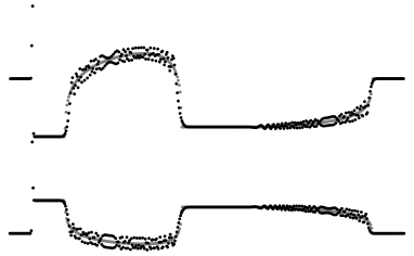
Figure 2: Solution of the Toda lattice (black) plus corresponding limiting lattice (gray). No gray points visible implies that black points overlap gray points.

The soliton was added using a Darboux transformation.

IV Conclusion

Let $g$ be the genus of the hyperelliptic Riemann surface associated with the unperturbed solution. We have shown that the $n/t$-plane contains $g+2$ areas where the perturbed solution is close to a quasi-periodic solution in the same isospectral torus. In between there are $g+1$ regions where the perturbed solution is asymptotically close to a modulated lattice which undergoes a continuous phase transition (in the Jacobian variety) and which interpolates between these isospectral solutions. In the special case of the free solution ($g=0$) the isospectral torus consists of just one point and we recover the classical result.

To conclude, we believe that, apart from the interesting mathematical problem of the analysis of Riemann-Hilbert problems on Riemann surfaces, the limiting lattice is interesting on its own. We even speculate that there may even be a physical or technological interest in such a modulated lattice and that the asymptotic problem described here might provide a feasible way of producing such modulated solutions.

- (1) P. Deift, X. Zhou, Ann. of Math. 137, 295–368 (1993).
- (2) B.A. Dubrovin, Russian Math. Surv. 36:2, 11–92 (1981).
- (3) I. Egorova, J. Michor, and G. Teschl, Comm. Math. Phys. 264, no. 3, 811–842 (2006).
- (4) I. Egorova, J. Michor, and G. Teschl, Inverse scattering transform for the Toda hierarchy with quasi-periodic background, Proc. Amer. Math. Soc. (to appear).
- (5) I. Egorova, J. Michor, and G. Teschl, Soliton solutions of the Toda hierarchy on quasi-periodic background revisited, in preparation.
- (6) S. Kamvissis, Comm. Math. Phys., 153, no. 3, 479–519 (1993).
- (7) S. Kamvissis, Physica D, 65, no. 3, 242–266 (1993).
- (8) S. Kamvissis and G. Teschl, Stability of the periodic Toda lattice under short range perturbations, in preparation.
- (9) E.A. Kuznetsov and A.V. Mikhaĭlov, Soviet Phys. JETP 40, no. 5, 855–859 (1975).
- (10) Yu. Rodin, The Riemann Boundary Problem on Riemann Surfaces, Mathematics and its Applications (Soviet Series), 16, D. Reidel Publishing Co., Dordrecht, 1988.
- (11) G. Teschl, Jacobi Operators and Completely Integrable Nonlinear Lattices, Math. Surv. and Mon. 72, Amer. Math. Soc., Rhode Island, 2000.
- (12) M. Toda, Theory of Nonlinear Lattices, 2nd enl. ed., Springer, Berlin, 1989.
- (13) N. J. Zabusky and M. D. Kruskal, Phys. Rev. Lett. 15, 240–243 (1963).