Spatial Distribution of Initial Interactions in High Energy Collisions of Heavy Nuclei

Abstract

The spatial distribution of interactions in high energy collisions of heavy nuclei is discussed using the wounded nucleon, binary collision, hard sphere, and colliding disk parameterizations of interaction densities. The mean radius, its dispersion, and the eccentricity of the interaction region are calculated as a function of impact parameter. The eccentricity is of special interest for comparison to measurements of anisotropic flow. The number of participants and binary collisions is also tabulated as a function of impact parameter.

1 Introduction

In this note we discuss the spatial distribution of initial interactions in the high energy collisions of heavy nuclei, in order to gain some insight into geometrical effects in such collisions. We apply a simple, widely used formalism (e.g. [1, 2]) that is often attributed to Glauber [3], to calculate the density of interactions projected onto the plane transverse to the beam axis for four commonly used weighting functions: number of wounded nucleons, number of binary collisions, colliding hard spheres, and colliding disks. The wounded nucleon and binary collision calculations incorporate the usual Woods-Saxon parametrization of nuclear density. We compute the mean and dispersion of the radius and the eccentricity of the interaction zone as a function of impact parameter for symmetric collisions of heavy nuclei. Using the same calculation we tabulate the number of participants for the wounded nucleon and hard sphere paramterizations, together with the number of binary collisions, as a function of impact parameter.

The distributions calculated are implicit in all model calculations of low or high sophistication that incorporate similar parameterizations of nuclear geometry, and in that sense nothing new is presented here. However, we have not found these distributions collected and discussed explicitly in the literature, and that is the the purpose of this note. A more detailed discussion of these and related results was presented previously in [4].

The formalism is described briefly in section 2. Section 3 discusses the transverse profile of the interaction volume as a function of impact parameter. Section 4 presents a parametrization of the eccentricity of the interaction region for non-central collisions. Section 5 tabulates the number of participants for the wounded nucleon and hard sphere paramterizations, together with the number of binary collisons, as a function of impact parameter.

2 Formalism

The coordinate system is defined in Figure 1. We utilize the standard nuclear thickness function $\mathrm{T}_{\mathrm{A}}$ [2],

$$\mbox{$\mathrm{T}_{\mathrm{A}}$}(|\vec{s}|)=\int{dz}\rho_{\mathrm{A}}(z,\vec{s}).$$ (1)

For the nuclear density we use a Woods-Saxon distribution,

$$\rho_{\mathrm{A}}(r)=\rho_{0}\cdot\frac{1}{1+e^{(r-\mbox{$\mathrm{R}_{\mathrm{A}}$})/\mathrm{a}}},$$ (2)

where $r=\sqrt{s^{2}+z^{2}}$, $\mbox{$\mathrm{R}_{\mathrm{A}}$}=1.12\cdot\mathrm{A}^{1/3}$, and $\rho_{0}=0.159$ GeV/$\mathrm{fm}^{3}$ and a=0.535 fm for $\ {}^{197}\mathrm{Au}$. $\rho_{\mathrm{A}}$ is normalized so that $\int{d^{2}s}\mbox{$\mathrm{T}_{\mathrm{A}}$}(|\vec{s}|)=\mathrm{A}$.

Figure 1: Transverse coordinate system. A and B are the masses of the colliding nuclei. The incoming beams are (anti-)parallel to the z axis. The x-z plane is commonly called the reaction plane.

In Fig. 1, the nuclear impact parameter is denoted b, and the distance to a point in the transverse plane from the center of either nucleus is denoted $\mathrm{b}_{\mathrm{A}}$ and $\mathrm{b}_{\mathrm{B}}$. The vector from the origin to this point is written

$$\vec{s}=\vec{\mbox{$\mathrm{b}_{\mathrm{A}}$}}-\frac{b}{2}\hat{x}=\vec{\mbox{$\mathrm{b}_{\mathrm{B}}$}}+\frac{b}{2}\hat{x}.$$ (3)

where $\hat{x}$ is the unit vector in the $x$ direction.

To calculate the density of interactions as a function of impact parameter for a given process, we utilize the limiting cases of high and low nucleon-nucleon cross section for that process:

• Wounded Nucleon Scaling: We consider the number of nucleons at $\vec{s}$ that are struck at least once by the nucleons in the oncoming nucleus, where “struck” means inelastically excited with nucleon-nucleon collision cross section $\sigma_{\mathrm{NN}}$. In the transverse projection, the density of wounded nucleons per nuclear collision is given in units $1/\mathrm{fm}^{2}$ by:

  $$\frac{\mathrm{d^{2}N}_{\mathrm{WN}}}{\mathrm{d}\mathrm{s}^{2}}=\mbox{$\mathrm{T}_{\mathrm{A}}$}(\mbox{$\mathrm{b}_{\mathrm{A}}$})\cdot(1-e^{-\mbox{$\mathrm{T}_{\mathrm{B}}$}(\mbox{$\mathrm{b}_{\mathrm{B}}$})\mbox{$\sigma_{\mathrm{NN}}$}})+\mbox{$\mathrm{T}_{\mathrm{B}}$}(\mbox{$\mathrm{b}_{\mathrm{B}}$})\cdot(1-e^{-\mbox{$\mathrm{T}_{\mathrm{A}}$}(\mbox{$\mathrm{b}_{\mathrm{A}}$})\mbox{$\sigma_{\mathrm{NN}}$}}),$$ (4)

  where the dependence on nuclear impact parameter is via Eq. 3.

• Binary Collision Scaling: More generally, we mean those processes with sufficiently small nucleon-nucleon cross section $\sigma_{\mathrm{NN}}^{\mathrm{hard}}$ that $(\mbox{$\mathrm{T}_{\mathrm{A}}$}\cdot\mbox{$\sigma_{\mathrm{NN}}^{\mathrm{hard}}$}){\ll}1$ (we apply the label “hard” because we are usually refering to high momentum transfer processes, or hard scattering). Nucleon-nucleon interaction probabilities can then be summed for the total interaction probability, and the number of hard scatterings per nuclear collision goes as the number of binary nucleon-nucleon collisions. The density in the transverse projection of hard processes per nuclear collision, in units $1/\mathrm{fm}^{2}$, is then

  $$\frac{\mathrm{d^{2}N}_{\mathrm{hard}}}{\mathrm{d}\mathrm{s}^{2}}=\mbox{$\sigma_{\mathrm{NN}}^{\mathrm{hard}}$}\cdot\mbox{$\mathrm{T}_{\mathrm{A}}$}(\mbox{$\mathrm{b}_{\mathrm{A}}$})\cdot\mbox{$\mathrm{T}_{\mathrm{B}}$}(\mbox{$\mathrm{b}_{\mathrm{B}}$}).$$ (5)

  Integrating over the transverse plane (and changing integration variables), the total number of hard processes per nuclear collision is given as a function of nuclear impact parameter b by[1, 2]:

  $$\mathrm{N}_{\mathrm{hard}}(b)=\mbox{$\sigma_{\mathrm{NN}}^{\mathrm{hard}}$}\cdot\int{d^{2}s}\mbox{$\mathrm{T}_{\mathrm{A}}$}(|\vec{s}|)\mbox{$\mathrm{T}_{\mathrm{B}}$}(|\vec{b}-\vec{s}|)\equiv\mbox{$\sigma_{\mathrm{NN}}^{\mathrm{hard}}$}\cdot\mbox{$\mathrm{T}_{\mathrm{AB}}$}(b)$$ (6)

3 Transverse Profile of the Interaction Volume for Non-central Collisions

The azimuthal anisotropy of momentum distributions in nuclear collisions can be related to the orientation of the event plane (the x-z plane in Figure 1) for noncentral collisions over a wide range of energies [5], and has been quantitatively studied up to the highest energy nuclear collisions at the SPS [6] and RHIC [7]. The lowest order harmonics are referred to as directed and elliptic flow, and are characterized by coefficients $\mathrm{v}_{1}$ and $\mathrm{v}_{2}$ respectively in a Fourier expansion of the azimuthal angle or momentum distributions [5].

Elliptic flow at midrapidity has received particular attention recently because of a possible connection to the Equation of State (see discussion and references in [5]). To help distinguish dynamics from purely geometrical effects, it has been suggested [8, 9] that the measured $\mathrm{v}_{2}$, the elliptic anisotropy, be scaled by the eccentricity of the reaction volume. This is defined to be [8, 9]

$$\epsilon\equiv\frac{<y^{2}>-<x^{2}>}{<y^{2}>+<x^{2}>}\approx\frac{b}{2\mbox{$\mathrm{R}_{\mathrm{A}}$}}$$ (7)

where $<\ldots>$ indicates the spatial average over the transverse plane weighted by a density such as that of wounded nucleons (equation 4). The approximation is the ratio of the lengths of the axes of the overlap region in Figure 1, $(y\mid_{x=0})/(x\mid_{y=0})$, not weighted by nuclear density [9].

We calculate the transverse density distribution of the reaction volume as a function of impact parameter, utilizing four different weighting functions:

• Wounded Nucleons: The transverse density profile is calculated using a Woods-Saxon density distribution and Eq. 4, appropriate for the bulk of particle production. We use $\sigma_{\mathrm{NN}}$=30 mb, but also investigate the sensitivity of the computed quantities to this parameter.

• Binary Collisions: The transverse density profile is calculated using a Woods-Saxon density distribution and Eq. 5, appropriate for hard processes such as jet and $\mathrm{J/}\Psi$ production.

• Hard Sphere: The transverse density profile is calculated for colliding sharp-edged spheres, with the density defined as $\mathrm{T}_{\mathrm{A}}$+$\mathrm{T}_{\mathrm{B}}$. This corresponds to the limit of the Wounded Nucleon density in which the Woods-Saxon parameter $a$ in Eq. 2 is small and $\sigma_{\mathrm{NN}}$ in Eq. 4 is large. The radius of the hard sphere corresponding to an Au nucleus is 7.24 fm, increased from the Woods-Saxon value of 6.52 fm in order to obtain the same total interaction cross section.

• Two Dimensional: The transverse density profile is simply the area of overlap region in Fig. 1, with uniform weighting (i.e. without taking into account the nuclear thickness in the z-direction and corresponding variation in density when projected onto the plane). The radius corresponding to a Au nucleus is 7.24 fm, as in the Hard Sphere calculation.

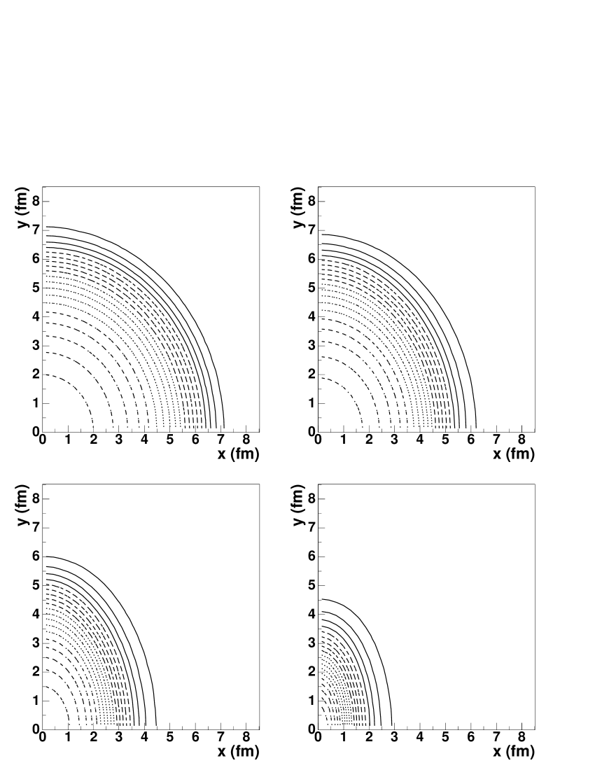
Figure 2: Transverse density of Wounded Nucleons as a function of (x,y) (see Fig 1), for collisions of Au+Au at impact parameters b=0, 4, 8 and 12 fm.

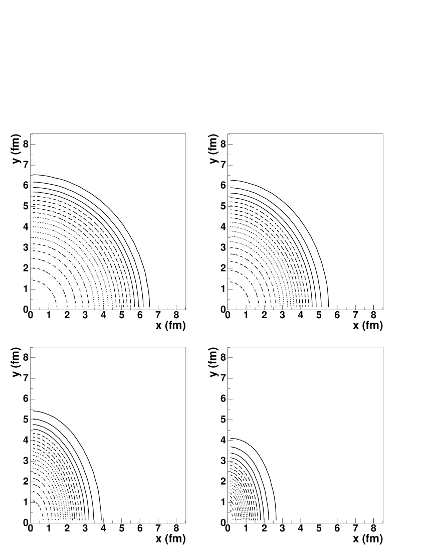
Figure 3: Transverse density of Binary Collisions as a function of (x,y) (see Fig 1), for collisions of Au+Au at impact parameters b=0, 4, 8 and 12 fm.

Figure 4: Transverse density profile of interacting hard spheres as a function of (x,y) (see Fig 1), corresponding to Au+Au at impact parameters b=0, 4, 8 and 12 fm.

Figure 5: Two dimensional transverse density profile as a function of (x,y) (see Fig 1) corresponding to the region of overlap in Fig 1, for Au+Au collisions at impact parameters b=0, 4, 8 and 12 fm.

We first present the transverse density profiles graphically, and then calculate moments to compare the distributions quantitatively. Figures 2 to 5 show the transverse density profiles for Au+Au collisions as linear contour plots in one quandrant of the coordinate system defined in Fig. 1, for the four weighting functions at different impact parameters. The Wounded Nucleon and Binary Collision profiles have very similar shape, with the Binary Collision distribution falling off slightly faster from the origin. The less realistic Hard Sphere and Two Dimensional calculations exhibit larger aspect ratios for noncentral collisions and unphysical sharp declines in the density at the boundaries of the overlap region.

Figure 6 shows the mean transverse radius ($<\!\mbox{$|\vec{\mathrm{s}}|$}\!>$ for Fig. 1) and its dispersion ($\sqrt{<\!\mbox{$|\vec{\mathrm{s}}|$}^{2}\!>-\mbox{$<\!\mbox{$|\vec{\mathrm{s}}|$}\!>$}^{2}}$) for the four weighting functions, as a function of impact parameter for Au+Au collisions. As is seen in the density profiles themselves, the Two Dimensional and Hard Sphere functions give larger mean radii than the Wounded Nucleon and Binary Collision functions. The dispersion in the radius is similar for all four functions, and is a weak function of impact parameter. The values at large impact parameter are dominated by the treatment of the nuclear surface.

Note that in the case of Binary Collision weighting, the mean (and median) radius is about 3.5 fm for the most central collisions. In other words, about one half of all produced e.g. $\mathrm{J/}\Psi$ or jets are generated farther than 3.5 fm. in the transverse plane from the center of the reaction zone in central collisions, with a distribution in radius which has a half-width of about 1.5 fm. Rather few of the $\mathrm{J/}\Psi$ or jets are produced near the center of the reaction, due simply to the geometry of nucleus-nucleus collisions.

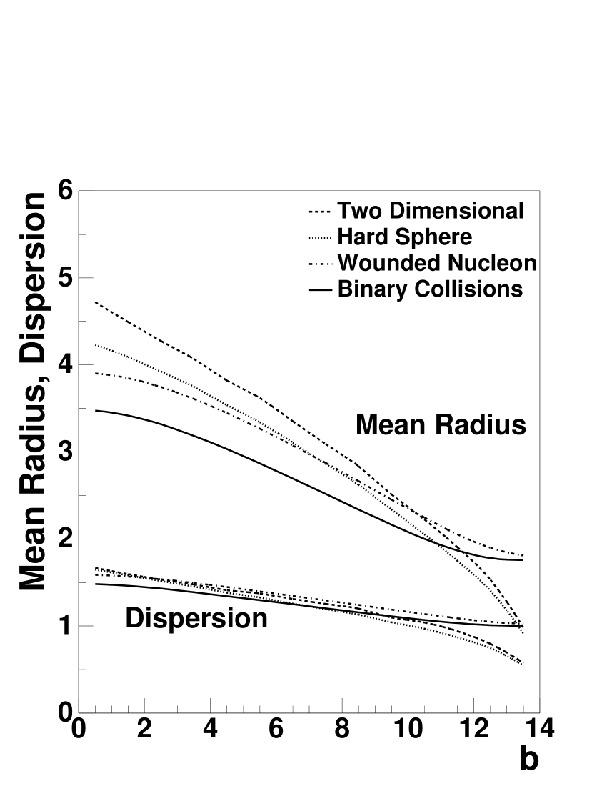
Figure 6: Mean and dispersion of radius of the interaction region as a function of impact parameter for Au+Au collisions, for the four weighting functions. The units of both axes are fm.

Figure 7 shows the eccentricity (Eq. 7) of the interaction region as a function of impact parameter for Au+Au collisions, for the four weighting functions. Also shown is the approximation b/(2$\mathrm{R}_{\mathrm{A}}$) from Eq. 7. The eccentricity of the Wounded Nucleon and Binary Collision models are similar and significantly smaller than those of the other models. Parametrization of $\epsilon$ in the Wounded Nucleon Model and its dependence upon $\sigma_{\mathrm{NN}}$ is given in the next section.

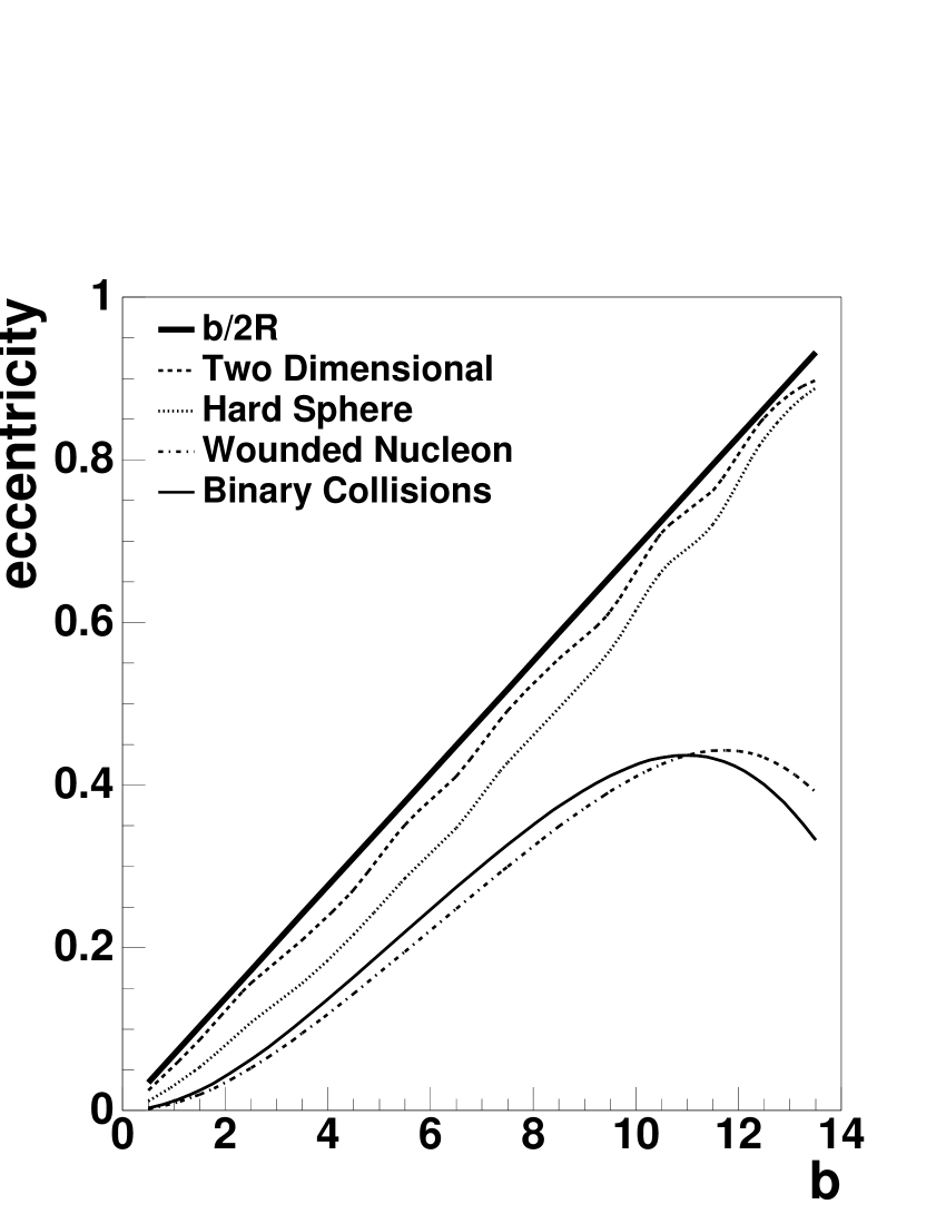
Figure 7: Eccentricity (Eq. 7) of the interaction region as a function of impact parameter for Au+Au collisions, for the four weighting functions.

4 Parametrization of $\epsilon$ and $S$ in the Wounded Nucleon Model

In this section we give a more detailed discussion of the characterization of the geometry of the interaction region in the Wounded Nucleon Model. The elliptic anisotropy of the overlap region $\epsilon$, defined in Eq. 7, is shown as a function of impact parameter in Fig. 7 for all four models for Au+Au collisions. $\epsilon$ is parametrized for the Wounded Nucleon Model ($\sigma_{\mathrm{NN}}$=30 mb) as

$$\epsilon(\mathrm{b})=-0.0469x+2.754x^{2}-4.797x^{3}+4.852x^{4}-2.492x^{5}$$ (8)

where $x=\mathrm{b}/(2\mathrm{R})$ and $2\mathrm{R}=15$ fm. for Pb+Pb collisions and $2\mathrm{R}=14.7$ fm. for Au+Au collisions.

Increase of $\sigma_{\mathrm{NN}}$ to 40 mb decreases $\epsilon$ by 13% at b=2.5 fm and 4% at b=10.5 fm, with the change monotonic in b. The decrease of $\epsilon$ with increasing $\sigma_{\mathrm{NN}}$ can be understood by noting that the value of $\epsilon$ is dominated by surface effects. Increasing $\sigma_{\mathrm{NN}}$ effectively extends the surface to larger radii, with the consequence that the shape of the interaction region in the transverse projection is less eccentric than for $\sigma_{\mathrm{NN}}$=30 mb at the same impact parameter.

For reference, we also include a parametrization in the same model of the impact parameter dependence of the quantity $S=\pi{R_{x}}{R_{y}}$ [9]. Here, $R_{x}=\sqrt{<\!x^{2}\!>}$, $R_{y}=\sqrt{<\!y^{2}\!>}$, and $<\!\ldots\!>$ denotes the spatial average used in Equation 7. In [9], $S$ is used to calculate the particle density in the overlap region. The parametrization is

$$S(\mathrm{b})/(\pi\mathrm{R}^{2})=0.164+0.0141x-0.684x^{2}+1.026x^{3}-0.763x^{4}+0.284x^{5}$$ (9)

where, again, $x=\mathrm{b}/(2\mathrm{R})$ and $2\mathrm{R}=15$ fm. for Pb+Pb collisions and $2\mathrm{R}=14.7$ fm. for Au+Au collisions.

b (fm)	# part	# part	# part (HS)	# BC ($\mu\mathrm{barn}^{-1}$)
	(WN, $\sigma_{\mathrm{NN}}$=30 mb)	(WN, $\sigma_{\mathrm{NN}}$=40 mb)
0.5	368	376	389	$2.8\cdot 10^{-2}$
1.5	355	364	366	$2.7\cdot 10^{-2}$
2.5	331	341	335	$2.5\cdot 10^{-2}$
3.5	298	310	302	$2.2\cdot 10^{-2}$
4.5	262	274	263	$1.8\cdot 10^{-2}$
5.5	223	234	226	$1.5\cdot 10^{-2}$
6.5	183	193	187	$1.2\cdot 10^{-2}$
7.5	144	155	148	$8.5\cdot 10^{-3}$
8.5	108	117	115	$5.8\cdot 10^{-3}$
9.5	77	84	82	$3.7\cdot 10^{-3}$
10.5	49	55	54	$2.1\cdot 10^{-3}$
11.5	28	32	32	$1.0\cdot 10^{-3}$
12.5	13	16	15	$4.0\cdot 10^{-4}$
13.5	5	6	4	$1.3\cdot 10^{-4}$

Table 1: Impact parameter dependence for Au+Au collisions of the number per nuclear collision of nucleon participants in the Wounded Nucleon model (columns 2 and 3) and colliding Hard Spheres (column 4), and the number of binary scatterings with cross section 1 $\mu$barn (column 5).

b (fm)	# part	# part	# part (HS)	# BC ($\mu\mathrm{barn}^{-1}$)
	(WN, $\sigma_{\mathrm{NN}}$=30 mb)	(WN, $\sigma_{\mathrm{NN}}$=40 mb)
0.5	388	397	410	$3.0\cdot 10^{-2}$
1.5	375	385	388	$2.9\cdot 10^{-2}$
2.5	351	362	358	$2.6\cdot 10^{-2}$
3.5	318	330	322	$2.3\cdot 10^{-2}$
4.5	281	293	286	$2.0\cdot 10^{-2}$
5.5	241	252	246	$1.6\cdot 10^{-2}$
6.5	199	211	206	$1.3\cdot 10^{-2}$
7.5	159	170	169	$9.5\cdot 10^{-3}$
8.5	121	131	132	$6.7\cdot 10^{-3}$
9.5	87	95	99	$4.3\cdot 10^{-3}$
10.5	58	64	69	$2.5\cdot 10^{-3}$
11.5	34	39	44	$1.3\cdot 10^{-3}$
12.5	17	20	23	$5.5\cdot 10^{-4}$
13.5	7	9	8	$1.9\cdot 10^{-4}$

Table 2: Impact parameter dependence for Pb+Pb collisions of the number per nuclear collision of nucleon participants in the Wounded Nucleon model (columns 2 and 3) and colliding Hard Spheres (column 4), and the number of binary scatterings with cross section 1 $\mu$barn (column 5).

5 Number of Participants and Binary Collisions

We conclude with a tabulation of the number of participants and binary collisions as a function of impact parameter. The distributions in Figures 2 to 4 can be integrated to calculate the total number of nucleon participants or binary collisions per nuclear collision. These are presented in Tables 1 and 2 for Au+Au and Pb+Pb collisions. Columns 2 and 3 give the number of Wounded Nucleons (Equation 4) with $\sigma_{\mathrm{NN}}$=30 and 40 mb. Column 4 gives the fraction of volume of the Hard Spheres that interact, normalized to the total number of incoming nucleons. Column 5 gives the number of binary collisions for an interaction cross section of 1 $\mu\mathrm{barn}$ (the rate for other small cross sections is obtained by linear scaling of this number).

Tables 1 and 2 show only a weak dependence of the number of participants on $\sigma_{\mathrm{NN}}$, and good agreement between the number of participants calculated with the Hard Sphere and Wounded Nucleon models. The latter point is in sharp contrast to the strong difference seen between the models for $\epsilon$ (Figure 7), and is due to the fact that the number of participants is dominated by the bulk volume, whereas $\epsilon$ is dominated by the surface overlap.

6 Acknowledgements

We thank Art Poskanzer, Raimond Snellings, and Sergei Voloshin for valuable discussions.

References

- [1] K. J. Eskola, K. Kajante and J. Lindfors, Nucl. Phys. B323, 37 (1989).
- [2] R. Vogt, nucl-th/9903051.
- [3] R.J. Glauber and G. Matthiae, Nucl. Phys. B21, 135 (1970); J. Hüfner and J. Knoll, Nucl. Phys. A290, 460 (1977); R. W. Hasse and W. D Meyers, “Geometrical Relationships of Macroscopic Nuclear Physics”, Springer Series in Nuclear and Particle Physics, Springer-Verlag, 1988.
- [4] P. Jacobs and G. Cooper, STAR Collaboration Internal Note SN0402.
- [5] R.J.M. Snellings, A.M. Poskanzer, and S.A. Voloshin, STAR Collaboration Internal Note SN0388, nucl-ex/9904003.
- [6] H. Appelshäuser et al. (NA49 Collaboration), Phys. Rev. Lett. 80, 4136 (1998).
- [7] STAR Collaboration, to be published.
- [8] H. Sorge, Phys. Rev. Lett. 82, 2048 (1999).
- [9] H. Heiselberg and A.-M. Levy, Phys. Rev. C59, 2716 (1999).