Charged Hadron Spectra in Au+Au Collisions at $\mbox{$\sqrt{s_{{}_{\mathrm{NN}}}}$}=130\ \mbox{$\mathrm{GeV}$}$

Abstract

The collision of high energy heavy ions is the most promising laboratory for the study of nuclear matter at high energy density and for creation of the Quark-Gluon Plasma. A new era in this field began with the operation and first collisions of Au nuclei in the Relativistic Heavy Ion Collider (RHIC) at Brookhaven National Laboratory during 2000. This work concentrates on measurement of global hadronic observables in Au+Au interactions at a centre-of-mass energy of $\mbox{$\sqrt{s_{{}_{\mathrm{NN}}}}$}=130\ \mbox{$\mathrm{GeV}$}$, which mainly address conditions in the final state of the collision. The minimum bias multiplicity distribution, the transverse momentum ($p_{\perp}$), and pseudorapidity ($\eta$) distributions for charged hadrons ($h^{-}$, $h^{+}$) are presented. Results on identified $\pi^{-}$ transverse mass ($m_{\perp}$) and rapidity ($y$) distributions are also discussed. The data were taken with the STAR detector with emphasis on particles near mid-rapidity.

We find that the multiplicity density at mid-rapidity for the 5% most central interactions is $dN_{h^{-}}/d\eta|_{\eta=0}=280\pm 1_{\textrm{stat}}\pm 20_{\textrm{syst}}$, an increase per participant of 38% relative to $p\bar{p}$ collisions at similar energy. The mean transverse momentum is $0.508\pm 0.012$ GeV/c and is larger than in $\mathrm{Pb}+\mathrm{Pb}$ collisions at lower energies. The scaling of the $h^{-}$ yield per participant nucleon pair, obtained via a ratio of $\mathrm{Au}+\mathrm{Au}$ to $p\bar{p}$ $p_{\perp}$ distributions, is a strong function of $p_{\perp}$. The pseudorapidity distribution is almost constant within $|\eta|<1$. The $\pi^{-}$ rapidity distribution is also flat around mid-rapidity in the region $|y|<0.8$, with a yield of pions for central collisions of $dN_{\pi^{-}}/dy|_{y=0}=287\pm 1_{\textrm{stat}}\pm 21_{\textrm{syst}}$. However, the slope of the $m_{\perp}$ distributions is not the same for different rapidity bins, suggesting that boost-invariance is not fully achieved in the collisions.

Charged Hadron Spectra in Au+Au Collisions at $\mbox{$\sqrt{s_{{}_{\mathrm{NN}}}}$}=130\ \mbox{$\mathrm{GeV}$}$

© Copyright 2024
by
Manuel Calderón de la Barca Sánchez
All Rights Reserved

Chapter 1 Introduction

Based on statistical Quantum Chromodynamics, our current expectation is that strongly interacting matter at extreme energy density ($\epsilon\gtrsim 1\ \mbox{$\mathrm{GeV}$}/\mbox{$\mathrm{fm}$}^{3}$) and temperature ($T\gtrsim 170\ \mbox{$\mathrm{MeV}$}$) is found in a state where hadrons no longer exist as discrete entities [1, 2]. The relevant degrees of freedom for such a system are those of the underlying partons, and we label this state the Quark-Gluon Plasma (QGP).[3, 4, 5, 6]

Such a state of matter is believed to be the one in which the early universe existed in a time scale $\sim 10^{-6}$ s after the Big Bang [7, 8] and is also predicted to exist in the interior of neutron stars [9, 10].

Ultra-relativistic heavy ion collisions are the most promising tool for the creation of a QGP in the laboratory. The appearance and study of predicted signatures in such collisions has been the subject of intense theoretical and experimental work for more than two decades (for recent reviews one can refer to the proceedings of the ‘Quark Matter’ conferences [11, 12, 13, 14, 15, 16, 17, 18, 19, 20, 21, 22, 23, 24, 25]). In the Alternating Gradient Synchrotron (AGS) at the Brookhaven National Laboratory (BNL) collisions have been produced using beams from Si to Au with energies of 11-14 $\mathrm{GeV}$ per nucleon. The corresponding centre-of-mass energy for $\mathrm{Au}+\mathrm{Au}$ collisions at the AGS is $\mbox{$\sqrt{s_{{}_{\mathrm{NN}}}}$}=5\ \mbox{$\mathrm{GeV}$}$. We use $\sqrt{s_{{}_{\mathrm{NN}}}}$ to denote the centre-of-mass energy per nucleon pair. The Super Proton Synchrotron (SPS) at the Conseil Européen de la Recherche Nucléaire (CERN) has yielded results from O, S and Pb beams with energies of 60-200 $\mathrm{GeV}$ per nucleon, this is a centre-of-mass energy of $\mbox{$\sqrt{s_{{}_{\mathrm{NN}}}}$}=17.2\ \mbox{$\mathrm{GeV}$}$ for $\mathrm{Pb}+\mathrm{Pb}$ collisions.

There has been considerable excitement in the field during the last year with the commissioning of the Relativistic Heavy Ion Collider (RHIC) at BNL [26]. Dedicated experiments began taking data in the summer of 2000 with the highest colliding energy heavy ion beams available. RHIC ran during this period with Au beams at a center of mass energy of $\mbox{$\sqrt{s_{{}_{\mathrm{NN}}}}$}=130\ \mbox{$\mathrm{GeV}$}$. Studying collisions at different energies helps to map the phase diagram of nuclear matter, where RHIC is expected to probe the region of high temperature and near-zero net-baryon density, a regime accessible by QCD lattice simulations.

For all heavy ion experiments, global event observables have played an important role. It remains true that to understand specific plasma signatures one must first understand the global character of the reaction dynamics. The momentum distribution of the bulk of the particles measured in the detectors provide evidence mainly of the final phase of the system formed in the collision, also called the freeze-out phase. In order to obtain information about the early stages where plasma formation is expected to occur, one must use indirect methods such as hard probes which must be gauged to reference observables related to the global character of the reaction. The information obtained in the final state in the form of particle spectra is one of the main sources of global event information. In addition, global final state observables help provide limits on the possible evolution of the system at earlier times. All experiments at RHIC and elsewhere have some capability to measure global observables in order to characterize and classify events, compare results with other experiments, and perform systematic studies. Measuring the final state particle spectra is therefore a basic requirement for the study of the collision dynamics.

The measurements of global observables for the first year of RHIC collisions are an exciting first topic of study in an energy regime where perturbative phenomena are expected to dominate. The contribution to the total charged particle multiplicity coming from hard processes (jets and mini-jets) at RHIC is estimated to be between $30-50\%$ [27, 28, 29, 30]. Since particle production is a dominant feature of the collision, one of the first observables to study is the multiplicity of charged particles for each event. This quantity and related global observables such as the transverse energy ($E_{\perp}$) and the energy deposition in the very forward region as measured typically by zero degree calorimeters (ZDCs) is related to the impact parameter of the collision. The more central the collision is, the more nucleons from both projectile nuclei will participate in the interaction, and hence the more secondary hadrons will be produced (large multiplicity and total $E_{\perp}$). A geometrical correlation between the impact parameter $b$, $E_{\perp}$ and the energy reaching the zero degree calorimeter can be given in terms of the number of “wounded” nucleons [31]. Central (high multiplicity) events have a special interest as it is for these events that the largest fraction of the incoming energy will be redistributed to new degrees of freedom. The next key observable is the distribution of the particles in momentum space. Rapidity and transverse momentum distributions allow one to address properties of the reaction dynamics such as the extent to which the nucleons are slowed down in the collision (stopping), the approach of the system to thermal equilibrium, and the shape of the emitting source of particles.

The Solenoidal Tracker At RHIC (STAR) is one of the 4 experiments that partake in the RHIC program. The analyses presented here are based on data taken by STAR during the 2000 summer run. The pith of the experiment is a large acceptance cylindrical Time Projection Chamber (TPC) placed in a uniform solenoidal magnetic field for momentum determination. The TPC provides charged particle tracking in the mid-rapidity region with full azimuthal coverage and particle identification for low momentum particles. The STAR detector is thus ideally suited for the study of hadronic observables and will therefore focus on such measurements early on, although the STAR physics program includes other topics in addition to QGP physics. Since hadrons are the most copiously produced particles in the collision and $\pi$ mesons comprise $\sim 80\%$ of the total hadron population, this work concentrates on the study of charged hadron ($h^{-}$ and $h^{+}$) and identified $\pi^{-}$ meson production and momentum spectra for $\mathrm{Au}+\mathrm{Au}$ collisions at $\mbox{$\sqrt{s_{{}_{\mathrm{NN}}}}$}=130\ \mbox{$\mathrm{GeV}$}$. The minimum bias $h^{-}$ multiplicity distribution is presented. For different selections of event centralities, we present the pseudorapidity ($\eta$) and transverse momentum ($p_{\perp}$) distributions for $h^{-}$. We compare the $p_{\perp}$ distributions to those expected in similar energy $p\bar{p}$ collisions as reference. We also discuss rapidity ($y$) and transverse mass ($m_{\perp}$) distributions for identified $\pi^{-}$.

This work is organized in the following manner. It starts with a discussion on general aspects of Quark-Gluon Plasma physics and a review of hadronic particle production at the AGS and SPS (chapters 2, 3 and 4), followed by a description of the STAR detector (chapter 5). An overview of the tracking strategy and detector calibration procedures is then given (chapter 6). After a discussion of the detector simulation (chapter 7) and a layout of the analysis technique and corrections (chapter 8), we present the results on hadron production and identified pion spectra and discuss their implications regarding the dynamics of the collision features at RHIC (chapters 9 and 10). Finally, we present our conclusions (chapter 11).

Chapter 2 The Physics of the Quark-Gluon Plasma

We give now an overview of the high temperature phase of QCD and the Quark-Gluon Plasma. For recent reviews on the subject, see e.g. [32, 33, 34], review articles in the proceedings of the ‘Quark Matter’ conferences  [35, 36] and the growing collection of books  [3, 5, 6, 37, 38].

2.1 Deconfinement in QCD

At the fundamental level, strongly interacting matter is described by interactions of quarks through the exchange of gluons. The theory that describes these interactions, quantum chromodynamics (QCD), has the remarkable properties that at large distances or small momenta $q$, the effective coupling constant $\alpha_{s}(q^{2})$ is large, and it decreases logarithmically at short distances or large momenta. This behaviour can be seen from perturbative QCD.

The QCD Lagrangian is given by

$$\mathcal{L}_{QCD}=i\bar{\psi}\gamma^{\mu}(\partial_{\mu}-ig\hat{A}_{\mu})\psi-m\bar{\psi}\psi-\frac{1}{4}F^{a}_{\mu\nu}F_{a}^{\mu\nu}$$ (2.1)

where the colour potential $\hat{A}_{\mu}$ is a $3\times 3$ matrix (indicated by the circumflex symbol) and can be represented by a linear combination of the 8 Gell-Mann matrices:

$$\hat{A}_{\mu}=\frac{1}{2}\sum_{a=1}^{8}A^{a}_{\mu}(x)\lambda_{a}\ .$$ (2.2)

This potential is introduced to make the Lagrangian invariant under local (space-dependent) rotations of the 3 colour components of the quark wavefunction $\psi$. The eight-component field strength tensor expressed as

$$F^{a}_{\mu\nu}=\partial_{\mu}A_{\nu}^{a}-\partial_{\nu}A_{\mu}^{a}+gf_{abc}A_{\mu}^{b}A_{\nu}^{c}\ ,$$ (2.3)

where $f_{abc}$ are the antisymmetric structure constants for the Lie group SU(3). The product $F^{a}_{\mu\nu}F_{a}^{\mu\nu}$ also remains invariant under a local colour gauge transformation.

The perturbative quantization proceeds in QCD in a similar manner as in Quantum Electrodynamics. The quadratic terms in the lagrangian define free quark and gluon fields, described by propagators with the same form as those in QED for electrons and photons. The free propagators $D_{0}(q^{2})$ are proportional to $1/q^{2}$, and if this were the only ingredient would lead to a colour force which would fall off like $1/r$. The main difference comes from the coupling of the gluon field to itself. This modifies the true gluon propagator, because one has to evaluate contributions arising from terms in the perturbation series corresponding to the virtual creation of a pair of coloured particles from the vacuum. We call this the ‘vacuum polarization’ function $\Pi(q^{2})$, and it turns out to be proportional to $-1/q^{2}\ln(-q^{2})$.

The higher order diagrams, in which the gluon interacts consecutively once, twice, three times with the vacuum polarization, etc. can be summed into a geometric series yielding the full propagator

$$D(q^{2}) = D_{0}(q^{2})+i^{2}D_{0}(q^{2})\Pi(q^{2})D_{0}(q^{2})+i^{4}D_{0}\Pi D_{0}\Pi D_{0}+\ldots$$ (2.4)

$$= \frac{D_{0}(q^{2})}{1-\Pi(q^{2})D_{0}(q^{2})}$$

$$= \left(1/q^{2}\right)\frac{1}{1+\frac{(33-2N_{F})\alpha_{s}}{12\pi\ln(-q^{2}/\mu^{2})}}$$

where $\mu$ is a reference point introduced by renormalization, and $N_{F}$ counts the number of flavours with mass below $|q^{2}|^{\frac{1}{2}}$. So after renormalization, the second factor in Eq. 2.4 acts as a momentum-dependent modification of the strong coupling constant. Combining it with $\alpha_{s}$ we obtain the “running” coupling constant

$$\alpha_{s}(q^{2})=\frac{4\pi}{(11-2N_{F}/3)\ln(-q^{2}/\Lambda^{2})}\propto\frac{1}{\ln(q^{2}/\Lambda^{2})}$$ (2.5)

where $\Lambda$ is a (dimensional) parameter introduced also by the renormalization process. We see that the running coupling exhibits a pole; in this approximation it is at $q^{2}=-\Lambda^{2}$. More sophisticated expressions for the gluon propagator indicate that the pole is really at $q^{2}=0$, and that $\alpha_{s}(q^{2})$ should behave as $1/q^{2}$ in the limit $q^{2}\rightarrow 0$.

Converted into coordinate space, this means that $\alpha_{s}(r)$ grows like $r^{2}$ for large distances, corresponding to a linearly rising potential. The logarithm in Eq. 2.5 causes a gradual decrease of the coupling strength between colour charges at large momenta or small distances. It is this property that is known as ‘asymptotic freedom’. This behaviour of the running coupling at large distances results in the confinement of quarks (i.e. isolated quarks are not observed in nature).

It is important to note that the behaviour of the strong coupling constant outlined above is derived for interactions in vacuo. The usual point of comparison for measurements and calculations of the strong coupling constant is at the mass of the $Z^{0}$ boson, $M_{Z}=91\ \mbox{$\mathrm{GeV/}c^{2}$}$, where the world average is $\alpha_{s}(M_{Z})=0.1172\pm 0.0045$ [39]. The typical initial momentum transfers at even the highest RHIC energies are significantly lower than $M_{Z}$, so we are really talking about a running of the coupling with temperature. One must instead focus on obtaining an expression for the coupling constant using expressions for the propagators which have corrections due to the presence of a coloured medium [3]. Using this modified propagator we again sum all diagrams with successive medium polarization functions $\Pi(q,T)$ to obtain an effective running coupling constant. Leaving aside the contribution of quark loop diagrams, this yields [3]

$$\alpha_{s}(q,T)=\frac{g^{2}}{4\pi(1-\Pi(q,T)/q^{2})}=\frac{4\pi}{11\ln(-q^{2}/\Lambda^{2})-48G(q/T)}$$ (2.6)

where

$$G(\zeta) = \int_{0}^{\infty}zdz\frac{f(z)}{e^{\zeta z}-1}\ \ \mathrm{and}$$

$$f(z) = (z-1/2z+1/8z^{3})\ln\left(\frac{|1-2z|}{|1+2z|}\right)-1+1/2z^{2}.$$ (2.7)

In the $q\rightarrow 0$ limit, the polarization function remains finite, which means that the propagator effectively contains a mass term, $D(q,T)=1/(q^{2}-\Pi(q,T))$, in a manner analogous to Debye screening in an electrolytic medium. This leads to the property that a test colour charge will cause a polarization of the charges in the coloured medium in the same way as electric charges in an electrolyte. In addition, an important property that follows from the temperature dependence of Eq. 2.6 is that as the temperature increases in QCD, the coupling becomes weak, falling logarithmically with increasing temperature. As a consequence, nuclear matter at very high temperature should not exhibit confinement.

Another important property that arises from the study of the QCD Lagrangian is that of chiral symmetry breaking (i.e. the quarks confined in hadrons do not appear as nearly massless constituents, but instead possess a mass of a few hundred $\mathrm{MeV}$ that is generated dynamically). The expectation value $\langle\bar{\psi}\psi\rangle\approx-(235\ \mbox{$\mathrm{MeV}$})^{3}$, usually called the quark condensate, describes the density of $q\bar{q}$ pairs found in the QCD vacuum, and the fact that it is non-vanishing is directly related to chiral-symmetry breaking. In the limit of zero current quark mass, the quark condensate vanishes at high temperature, i.e. chiral symmetry is restored. It is this phase of QCD which exhibits neither confinement nor chiral-symmetry breaking that we entitle the Quark-Gluon Plasma.

Since the quark condensate is zero in the high temperature phase and non-zero at low temperature, it therefore acts as an order parameter. This behaviour leads to the expectation that the change between the low-temperature and high-temperature phases should exhibit a discontinuity. For 2 (3) massless quark flavours, universality arguments predict a second- (first-) order phase transition [40, 41]. The question of the order of the transition, or if there is a phase transition as opposed to a rapid cross-over, for QCD with the real values for the $u$, $d$ and $s$ quark masses is still the subject of current investigations [42, 43].

2.1.1 Phase Diagram

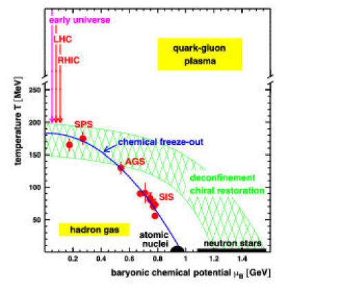
Figure 2.1: Phase diagram of hadronic matter, showing hadron gas and quark-gluon plasma regions. The temperature $T$ and the baryochemical potential $\mu_{B}$ data are derived from particle yield ratios. The solid curve through the data points represents the chemical freeze-out of hadronic-matter.

One of the first pictures that can serve as a guide to the behaviour of QCD can be obtained from the simplified ‘MIT bag model’ [44]. We can identify two regions where we expect deconfinement to occur: when compression causes the hadrons to overlap significantly, reaching densities 3 to 5 times higher than those of ordinary nuclear matter (0.17 $\mbox{$\mathrm{fm}$}^{-3}$), or when the temperature of the medium exceeds some critical threshold. Figure 2.1 shows the usual representation of the ‘$T-\mu_{B}$’ phase diagram, where $\mu_{B}$ is the Baryon chemical potential. It is normally represented with a continuous curve connecting the high temperature transition region at $\mu_{B}=0$ with the high baryon density region at $T=0$. The figure shows the regions probed by the different beam energies from the SIS to RHIC. At high densities and near-zero temperature we expect a deconfined phase. This deconfined high-density phase is predicted to exist for example in the interior of neutron stars. The near-zero Baryon chemical potential and high temperature region is the one probed by the highest energy RHIC collisions. The region where $\mu_{B}=0$ is believed to be the one in which the early universe existed, and is also accessible to numerical simulations of QCD on a lattice. The data points in the figure are from an analysis of particle ratios which is customarily employed to evaluate the degree of chemical equilibration observed in the final state. To roughly illustrate the region that is probed by RHIC in the diagram, preliminary analysis from mid-rapidity particle ratios at RHIC [45] indicate a value of $\mu_{B}\simeq 0.050\ \mbox{$\mathrm{GeV}$}$ and of the chemical freeze-out temperature of $T_{\mathrm{ch}}\simeq 170\ \mbox{$\mathrm{MeV}$}$. We discuss chemical and kinetic freeze-out in Chapter 3. It should be noted however, that we do not really know where the transition curve really lies, or even if there is a transition as opposed to a rapid cross-over at finite baryon number density. First principle numerical calculations of QCD, discussed in the next section, have provided us with guidance, but most results so far pertain to the $\mu_{B}=0$ region.

2.2 Lattice QCD Results

From sophisticated numerical simulations of QCD on the lattice, we have gained much insight into the structure of the QCD at high temperature.

The approach is based on the Feynman path integral: the aim is to calculate the action on the lattice and use it to evaluate expectation values of different observables. The first results used pure SU(3) gauge theory, sometimes called pure glue theory. A problem arises when one introduces the (discrete) fermion fields in a straightforward way, one obtains a ‘doubling’ of the flavour spectrum in the quark sector. We get $2^{d}=16$ copies of each quark species (in $d=4$ dimensions). Different approaches were then introduced to incorporate the fermion degrees of freedom in a way that reduces the doubling problem. The approach proposed by Wilson [46] solves the flavour doubling essentially by giving the doublers a mass proportional to 1/$a$, where $a$ is the lattice spacing, so they go away in the continuum limit. The disadvantage is that the mass introduces a chiral-symmetry breaking piece into the action. Another action known as the Kogut-Susskind[47], or also as the ‘staggered’ fermion action[48, 49], has the advantage of preserving a part of chiral symmetry. However, it does not completely eliminate the flavour problem. The number of doublers is reduced to 4. This leads for example to having $4^{2}-1=15$ pions instead of the usual $2^{2}-1=3$. In addition, the Wilson action yields results that in general need corrections of $\mathcal{O}(a)$, where $a$ is the lattice spacing, whereas the staggered fermion action is fine up to $\mathcal{O}(a^{2})$.

In the last decade, there have been significant developments that provide a solution to the doubling problem. The “domain wall” [50] approach relies on introducing a fifth (fictitious) dimension such that the chiral zero modes live on 4D surfaces. If $N_{5}$ is the number of lattice spacings along the fifth dimension, in the limit $N_{5}\rightarrow\infty$ the left- and right-handed fields live in surfaces in opposite ends of the 5D lattice and do not mix, so we have exact chiral symmetry with no doublers. An alternative approach has been presented where chiral symmetry is preserved in the lattice if the lattice Dirac operator is of a certain form (see e.g. Ref. [51]). Although several constructions for the Dirac “overlap” operator exist, they all satisfy an identity, originally due to Ginsparg and Wilson [52], which guarantees having exact global chiral symmetries directly on the lattice. For a recent review of the overlap approach, see e.g. Refs. [53, 54].

2.2.1 Critical Temperature and Energy Density

Over recent years, thermodynamic calculations on the lattice have steadily been improved. This is partly due to the much improved computer resources, however equally important has been (and will continue to be) the development of improved discretization schemes, i.e. improved actions.

Early calculations of the QCD transition temperature performed with standard Wilson fermions [46, 55] and staggered fermion actions [49] led to significant discrepancies of the results. These differences were greatly reduced based on improved Wilson fermions (Clover action) [56, 49, 57], as well as improved staggered fermions [58, 42], and domain wall [50] approaches. We shall not discuss these here, but only take the current results from improved staggered fermion actions for the following discussion.

Typically, one can look at the dependence of the energy density $\epsilon$ and pressure versus temperature where one expects a change due to the increase in the number of degrees of freedom (d.o.f.). In order to illustrate this point, we can obtain some semi-quantitative insight into the number of degrees of freedom and the energy density using the following simplified scenario. A massless non-interacting hadron gas is made up basically of pions, of which we have 3 types ($\pi^{+}$, $\pi^{-}$, $\pi^{0}$) neglecting the resonances. From an ideal relativistic Bose gas at Temperature $T$ we obtain the energy density

$$\epsilon_{g}=\int\frac{d^{3}p}{(2\pi)^{3}}\frac{p}{e^{p/T}-1}=\frac{4\pi T^{4}}{(2\pi)^{3}}\int_{0}^{\infty}\frac{x^{3}\ dx}{e^{x}-1}dx=\frac{\pi^{2}}{30}T^{4}\ ,$$ (2.8)

where we have rescaled the momentum as $x=p/T$. This is the usual Stefan-Boltzmann relation ($\epsilon=aT^{4}$). The energy density for the hadron gas is therefore simply

$$\epsilon_{HG}=3\ \epsilon_{g}=3\ \frac{\pi^{2}}{30}T^{4}\ .$$ (2.9)

For a QGP consisting of 2 massless quark flavours ($u$ and $d$) at vanishing net baryon density ($\mu=0$) we must sum the quark and the gluon contributions to the energy density. The gluon contribution is given by Eq. 2.8 times the 16 gluonic d.o.f. ($2_{\mathrm{spin}}\times(3^{2}-1)_{\mathrm{colour}}$). The quark contribution is obtained from a similar integral for a Fermi gas

$$\epsilon_{q}=\int\frac{d^{3}p}{(2\pi)^{3}}\frac{p}{e^{p/T}+1}=\frac{4\pi T^{4}}{(2\pi)^{3}}\int_{0}^{\infty}\frac{x^{3}\ dx}{e^{x}+1}dx=\frac{7}{8}\frac{\pi^{2}}{30}T^{4}\ .$$ (2.10)

Multiplying by the number of (anti)quark d.o.f. ($2_{\mathrm{spin}}\times 3_{\mathrm{colour}}\times N_{F}$) we obtain the energy density

$$\epsilon_{QGP}=16\epsilon_{g}+6N_{F}(\epsilon_{q}+\epsilon_{\bar{q}})=16\frac{\pi^{2}}{30}T^{4}+12N_{F}\frac{7}{8}\frac{\pi^{2}}{30}T^{4}=(16+\frac{21}{2}N_{F})\frac{\pi^{2}}{30}T^{4}\ .$$ (2.11)

Figure 2.2 shows recent results for the energy density $\epsilon$ as a function of temperature in lattice QCD simulations with $N_{F}$ = 0, 2 and 3 light quarks as well as two light and a heavier (strange) quark (2+1 flavour QCD). The pressure $p$ is shown in Figure 2.3a for QCD with different number of flavours as well as for the pure SU(3) gauge theory. The curves clearly reflect the strong change in the number of degrees of freedom when going through the transition. In the high temperature limit ($T\gtrsim 1.5\ \mbox{$T_{c}$}$), we expect both $\epsilon$ and $p$ to asymptotically approach the Stefan-Boltzmann free gas limit Eq. 2.11, indicated by the arrows in the figures. From the figure, it is evident that even at $4\mbox{$T_{c}$}$ the Stefan-Boltzmann limit is not reached. This has been taken as indication of a significant amount of interactions among partons in the high temperature phase, with only a logarithmic approach to the free-gas behaviour.

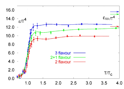
Figure 2.2: Energy density $\epsilon$ obtained from a numerical evaluation of QCD on the lattice [42]. $\epsilon$ is divided by $T^{4}$ to exhibit the sudden rise of the number of thermally excited degrees of freedom near the critical temperature $T_{c}$. Arrows show the ideal gas values as given by Eq. 2.11.

In addition, the dependence of $T_{c}$ on the number of partonic degrees of freedom is clearly visible in Figure 2.3a. It is therefore striking that $p/p_{SB}$ is almost flavour independent when plotted in units of $T/\mbox{$T_{c}$}$ as shown in Figure 2.3b.

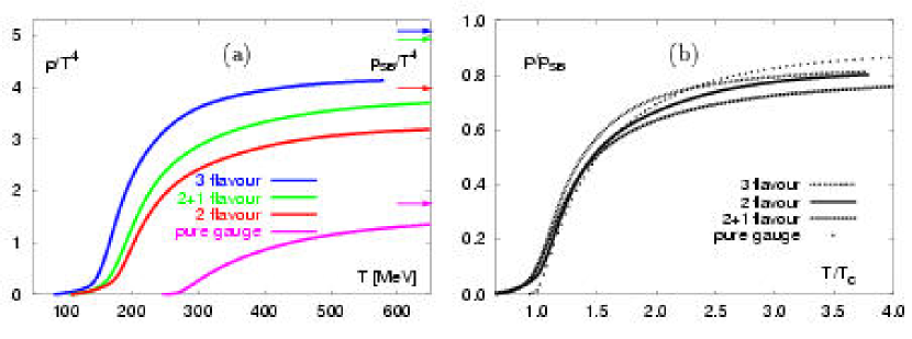
Figure 2.3: The Pressure $p$ in lattice QCD [42]. Left panel: Curves with $N_{F}=0,2\ \mathrm{and}\ 3$ light quarks as well as the “(2+1)” case. Right panel: $T$ axis scaled by the value of $T_{c}$ for each curve.

The most recently reported results on the value of $T_{c}$ from lattice calculations are found to be, for one particular choice of actions (improved staggered fermion action) [43]

$$N_{F}=2 : \mbox{$T_{c}$}=173\pm 8\mbox{$\mathrm{MeV}$}\$$

$$N_{F}=3 : \mbox{$T_{c}$}=154\pm 8\mbox{$\mathrm{MeV}$}\ .$$ (2.12)

The results also suggest that the transition temperature in (2+1)-flavour QCD is close to that of 2-flavour QCD.

The behaviour of the different actions (improved staggered, Wilson, Clover, etc.) currently studied in lattice QCD should show agreement in the vicinity of the phase transition. In this regime, the correlation lengths become large and cut-off effects in the calculations become less important. One can therefore compare calculations made with different actions. In particular, the recent results for the energy density at $T_{c}$ yield

$$\epsilon_{c}\simeq(6\pm 2)\mbox{$T_{c}$}^{4}=0.70\pm 0.23\ \mbox{$\mathrm{GeV}$}/\mbox{$\mathrm{fm}$}^{3}.$$ (2.13)

as shown in Figure 2.2 by the vertical line at $T=\mbox{$T_{c}$}$. It is important to stress that these values refer to initial energy densities, when the medium exists at the early stages of QGP evolution, and must be translated into a final energy density that can be measured in an experiment using detected particles. Bjorken [59] introduced a relation to address this question. One can experimentally estimate the energy density achieved in a nucleus-nucleus collision via the energy measured in the central rapidity region, $d\mbox{$E_{\perp}$}/dy$, divided by the effective interaction volume, ($A_{T}\cdot\tau$). In this case, we estimate the energy by a product of the particle multiplicity $(\mbox{$dN/dy$}|_{y=0})$, times the mean transverse mass of the particles, ($\langle m_{\perp}\rangle$).

$$\epsilon=\frac{\frac{dN}{dy}\arrowvert_{y=0}\cdot\mbox{$\langle m_{\perp}\rangle$}}{A_{T}\cdot\tau}\ .$$ (2.14)

In this expression, the factor $A_{T}$ is the transverse area of overlap in the collision. The quantity $\tau$ is less accurately defined. It is normally interpreted as the parton formation time, i.e. the time needed to pass from the initial hadronic environment to the partonic degrees of freedom. Usually, this time is taken as 1 $\mbox{$\mathrm{fm}$}/c$ at SPS in order to compare different experiments. However, there is currently no real consensus as to what is the appropriate formation time $\tau$ to use at RHIC, although if anything there are arguments that it should be smaller than 1 $\mbox{$\mathrm{fm}$}/c$ at high energies  [60] because it should take less time to equilibrate the system. An estimate of the energy density using this relation should then be at best considered a lower limit (with respect to this formation time).

For reference, in the case of STAR, this relation can be calculated for a given centrality selection, we choose the 5% most central collisions, using the total charged multiplicity and the transverse momentum distribution for charged particles (Sec. 9.3, and  9.2 respectively). The transverse area $A_{T}$ can be computed in a geometrical model that reproduces the measured multiplicity distribution (Sec.  4.1.1). Equation 2.14 is a very accessible experimental observable, but there are additional caveats associated with its interpretation of which the formation time is but one example. We discuss the applicability and additional uncertainties associated with equation 2.14 in Section 9.3.

2.2.2 Heavy Quark Effective Potential

In the lattice approach, an interesting quantity one can calculate is the effective potential between two heavy quarks, for it is the example which most cleanly illustrates the modification of the behaviour of the coloured fields at high temperature. From the previous section, we delineated the behaviour of the strong coupling constant: at large momenta or small distances it should be small and at small momenta or large distances the coupling rises as $1/q^{2}$ (asymptotic freedom). This leads to an effective potential that rises linearly with $r$, the distance between the coloured constituents, and can be calculated in the lattice.

Figure  2.4 shows the results of a lattice calculation for the heavy quark potential as a function of distance.

 

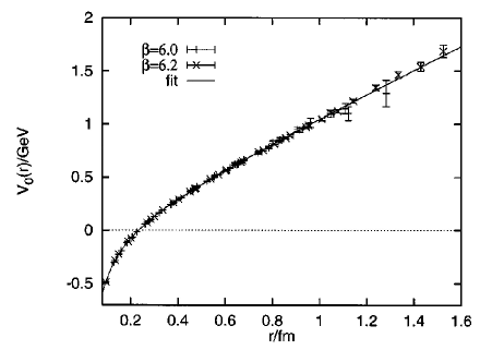
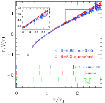
Figure 2.4: The heavy quark effective potential as a function of distance $r$ in lattice QCD. The left panel shows a quenched ($N_{f}=0$) calculation using Wilson loops, in physical units. The right panel shows a comparison between a quenched calculation (red) and one including quark loop effects (blue) showing nice agreement. Vertical bars near the horizontal axis show the scale of the lattice spacing $a$, and intervals in physical units 0.1 $\mathrm{fm}$ wide for reference. Figures are from Refs. [61] (a) and [62](b).

We see the potential is very weak at small distances and the expected linear rise at large distances. The slope of the linear rise is usually called the string constant, since it can be thought of as the tension of a spring.

One can test the idea of deconfinement at high temperature in lattice calculations in a straightforward way. As we raise the temperature, one can study the behaviour of the effective potential. We expect that near the critical temperature, the linear piece of the potential should be modified and weakened. At high temperature, the energy cost to create light $q\bar{q}$ pairs from the vacuum is reduced (this is related to the vanishing of the quark condensate and the restoration of chiral symmetry in the $T>T_{c}$ phase of QCD). These light $q\bar{q}$ pairs then act as screening colour charges around the heavy quark pair, thus weakening the potential.

Figure  2.5 shows the heavy quark potential for different temperatures in the region near $T_{c}$.

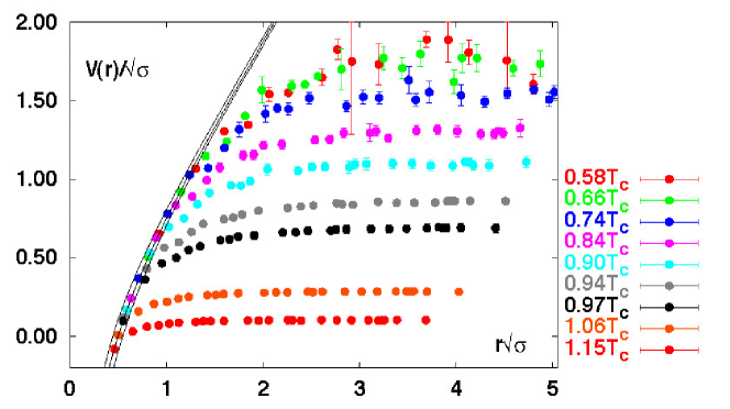
Figure 2.5: The heavy quark effective potential for different temperatures, taken from Ref. [42]. The linear rise of the potential is weakened as one approaches the critical temperature. The solid curves show the Cornell potential $V(r)=-\alpha/r+\sigma r$ with $\alpha=0.25\pm 0.05$, which is used to normalize the finite temperature free energies at the shortest distance available, $r=1/(4T)$.

It is clear that there are important modifications to the strength of the potential at high temperatures. We see that as the temperature increases, the strength systematically decreases. The potentials in Figure  2.5 also do not show the steep rise as in the quenched case. This is an expected phenomenon that had proved elusive in lattice calculations. As the quark-antiquark pair separate, we expect the formation of a tube of flux, or string, which should break in the presence of light quark-antiquark pairs. The results in the figure show that the string does in fact break in the confining phase at non-zero temperature. The weakening of the potential at high temperature has important consequences for heavy quark bound states. In particular, it is this behaviour that is the basis for the concept of J/$\psi$ suppression in a deconfined medium  [63].

We next need to address how we can measure the properties of excited hadronic and partonic matter in the laboratory and how can we hope to see a signal of QGP formation. We therefore proceed to discuss the experimental side of QGP physics.

Chapter 3 Experimental Search for the QGP

The use of beams of heavy elements allows us to distribute the incoming energy over an extended region of space, large compared to the size of one nucleon, with the hope of creating conditions that are suitable for the formation of a QGP. One can identify the following phases, shown schematically in Fig. 3.1:

 

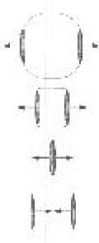
Figure 3.1: 1-D Space-time picture of the evolution of an ultra-relativistic nuclear collision, distinguishing 3 regions: (a) Pre-equilibrium state, (b) thermalized QGP, (c) hadronization stage. (see text). The $z$ axis denotes the beam direction, and the dashed lines indicate the colliding nuclei near the light-cone region.

i) The interpenetration of the nuclei with partonic interactions at high energy. This stage features the creation of e.g. high-$p_{\perp}$ jets, $c\bar{c}$ pairs or other products of high momentum transfer scattering processes on the parton level. In addition, large cross-section soft nucleon nucleon scattering between the two highly Lorentz-contracted nuclei help redistribute a fraction of the incoming kinetic energy into other degrees of freedom. The small cross-section hard processes are used as experimental probes for the hot and dense zone.

ii) The interaction of the particles of the system, driving it towards chemical and thermal equilibrium. Partons materialize out of the highly excited QCD field. If QGP forms, the quark mean free path at energy densities $\epsilon=2\ \mbox{$\mathrm{GeV}$}/\mbox{$\mathrm{fm}$}^{3}$ is $\lambda\approx 0.5\ \mbox{$\mathrm{fm}$}$, and individual parton-parton scattering is expected to play a role in thermalizing the system during this early stage as the nuclear dimensions are larger than $\lambda$. The interactions also originate the development of collective flow. Rapid expansion, mainly along the longitudinal direction, lower the temperature of the system eventually reaching the cross over temperature $T_{c}$. Direct photon signals from the QGP are generated from collisions of charged particles during the expansion stage, although there are also photon signals from the hot hadron gas stage. Final formation of charmonium states (J/$\psi$, $\psi\prime$) from the initial $c\bar{c}$ pairs happens also during this stage.

iii) The hadronization stage and the ‘freeze-out’ of the final state particles is then reached at $T<\mbox{$T_{c}$}$, as the system cools down so that there is not enough energy in each collision to further change the different species’ populations or ratios (chemical freeze-out, $T\sim 160-170\ \mbox{$\mathrm{MeV}$}$). Eventually, the energy is small enough and the system dilute enough such that the interactions cease and the momentum spectra do not change further (kinetic freeze-out, $T\sim 120\ \mbox{$\mathrm{MeV}$}$). To obtain information of the different stages, experimentally one must start from the measurement of final state particles. Global observables are useful to determine the initial conditions such as centrality, initial volume, and possibly energy density.

There are some observables that also provide information from the early stages. Signals such as direct photons and dilepton pairs that originate during early times are interesting since they are little disturbed by the hadronic final state. The caveat in studying such signals is that they typically have a much smaller cross section compared to hadronic observables.

There are also a class of hadronic observables that are thought to be sensitive to early times. In particular, the measurement of an azimuthal anisotropy in the emission of particles (with respect to the reaction plane, i.e. the plane formed by the beam direction and the direction of a vector connecting the center of the two colliding nuclei) is one example. In non-central collisions, an initial spatial anisotropy would result in pressure gradients which drive the emission of particles, producing a modulation in the azimuthal distribution of particles with respect to the reaction plane. This effect is typically measured by a Fourier analysis of the azimuthal particle distribution, where the 2nd Fourier component is called elliptic flow (in reference to the picture of particles in a fluid moving under the influence of the initial pressure gradient) and is denoted as $v_{2}$. The STAR experiment [64] already measured the charged particle elliptic flow signal at low $p_{\perp}$, and from these results we already see evidence of significant collective behaviour during the early stages of collisions at RHIC energies.

3.1 QGP Signatures

Many different effects have been proposed as possible ways to detect experimentally the formation of the QGP state of matter. These range from the earliest and most naïve studies which involved plotting mean $p_{\perp}$ ($\langle p_{\perp}\rangle$) as a function of particle multiplicity as a quick way to look into the structure of the $T-\epsilon$ phase diagram [65], to the more current searches for modification of particle properties (enhancement, suppression or medium-induced changes in mass or width), and the statistical studies of charge (or other observable) fluctuations event-by-event. While some probes give information primarily about ‘surface’ effects, like the hadrons’ $p_{\perp}$ distributions discussed here, strangeness production and particle interferometry which reveal final state information; some others deal with deeper ‘volume’ effects which are sensitive to early times after the collision. These include most ‘hard’ processes, i.e. those which involve large momentum transfers, for example charm and beauty production ($J/\psi$, D mesons, $\Upsilon$), jets and high-$p_{\perp}$ particle production. Usually, the attention is on ‘volume’ probes that address the features of the QGP itself, i.e. those probes which provide more direct information from the hot and dense phase of the reaction and are not influenced much by the high number of hadrons produced in the collision (e.g. by hadronic rescattering). This is the ideal case, but the experience has been that one must carefully study the modification of the proposed signals by conventional nuclear means (i.e. non-QGP). It is also important to emphasize that all of the different clues must be investigated as a function of the associated particle multiplicity or equivalent probe giving information on global characteristics. One would like to understand the onset of all of the observed signals in terms of the different handles at our disposal. Experimentally we can vary the collision centrality (selecting on multiplicity or transverse energy), we can collide different nuclear species (a more controlled variation of system size) and we can vary the centre-of-mass energy. The experimental data will in turn help to constrain the theoretical model parameters and input (e.g. equation of state, expansion dynamics and collective flow, size and lifetime of the system for hydrodynamical models; and initial parton densities, parton mean-free path and cross section, nuclear shadowing of initial parton distributions, and amount of parton energy loss in the plasma for perturbative approaches). For example, using hadron and electromagnetic spectra from several SPS experiments, attempts have been made to constrain the equation of state and initial conditions in a hydrodynamical approach [66].

In the following we will briefly mention some of the experimental signals that have been proposed to probe the system created in heavy ion collisions. For a recent review on QGP signatures, see Ref. [34].

3.1.1 Charmonium Suppression

The arguments for charmonium suppression were laid out in Section 2.2.2. Essentially, the weakening of the heavy quark effective potential with increasing temperature, or alternately viewed as the Debye screening of free colour charges in a QGP, is responsible for the breakup of charmonium states [63]. Excited states of the $c\bar{c}$ system, such as $\psi\prime$ and $\chi_{c}$, are easier to dissociate due to their larger radii, and are expected to dissolve just above $T_{c}$. The smaller J/$\psi$ becomes unbound at a higher temperature, $T\gtrsim 1.2\mbox{$T_{c}$}$. Similar arguments apply to the dissociation of the heavier $b\bar{b}$ bound states, but they require much shorter screening lengths to dissolve, i.e. greater temperature and energy densities [67]. The $\Upsilon$ state may dissolve above a temperature of $\sim 2.5\mbox{$T_{c}$}$, while the $\Upsilon^{\prime}$ could also dissolve near $T_{c}$.

“Anomalous” J/$\psi$ suppression has been reported by the NA50 collaboration for central $\mathrm{Pb}+\mathrm{Pb}$ collisions at SPS which has been heralded as evidence for QGP formation [68, 69, 70]. There are nuclear effects, such as the breakup of the J/$\psi$ by hadronic comovers, which also suppress the measured cross section in nucleus-nucleus collisions [71]. This issue is still one of intense debate, with many journal publications devoted to the topic. There are already some model predictions on J/$\psi$ suppression at RHIC and LHC energies based on normal nuclear effects, such as $p_{\perp}$ broadening and nuclear shadowing of the parton distribution functions [72]. Such an analysis lead for example to anti-shadowing at RHIC energies, i.e. the modifications introduced by cold nuclear matter enhance quarkonium production at RHIC (at LHC the opposite occurs). It has become clear that several mechanisms need to be considered in order to fully comprehend quarkonium production and suppression: the underlying physics description at different energies (hadronic at AGS and SPS, partonic at collider energies), nuclear effects such as shadowing, interaction with comovers, J/$\psi$ production due to the decay of higher mass resonances, and the signals from $pA$ data. For the most recent developments, one can see for example the talks in the dedicated J/$\psi$ session at Quark Matter ’01 [25], where suppression from the comover mechanism [71], a model based on $E_{\perp}$ fluctuations for the most central events to explain the NA50 $\mathrm{Pb}+\mathrm{Pb}$ data [73], and even enhancement of J/$\psi$ production in deconfined matter at RHIC energies [74] were discussed.

3.1.2 Jet Quenching

The colour structure of QCD matter can be probed by its effect on the propagation of a fast parton. The mechanisms are similar to those responsible for the electromagnetic energy loss of a fast charged particle in matter: energy may be lost either by the excitation of the penetrated medium or by radiation . The QCD analog of this effect indicates that the stopping power of the Quark-Gluon Plasma should be higher than that of ordinary matter [75]. This effect is called jet quenching [76, 77] and has several consequences that could be observable in experiments. Of more direct relevance to particle spectra, a comparison of the transverse momentum spectrum of hadrons compared to appropriately scaled distributions from $pp$ or $p\bar{p}$ collisions should show a suppression at high-$p_{\perp}$ ($\gtrsim 4$ $\mathrm{GeV/}c$). In addition, a quark or gluon jet propagating through a dense medium will not only lose energy, it will also be deflected. This will destroy the coplanarity of the two jets with respect to the beam axis. The angular deflection in addition leads to an azimuthal asymmetry. One can then perform angular correlations among high $p_{\perp}$ particles to study the energy loss effects of the partons in the medium.

3.1.3 Medium Effects on Hadron Properties

The widths and masses of the $\rho$, $\omega$ and $\phi$ resonances in the dilepton pair invariant mass spectrum are sensitive to medium-induced changes, especially to possible drop of vector meson masses preceding the chiral symmetry restoration transition. The CERES data from S+Au and Pb+Au collisions at SPS showed an excess of dileptons in the low-mass region 0.2 < $M$ < 1.5 $\mathrm{GeV/}c^{2}$, relative to $pp$ and $pA$ collisions [78, 79], which has been the subject of active discussion. Although the CERES data can be explained by a hydrodynamic approach assuming the creation of a QGP [80], alternative scenarios have also provided explanations. These have included for example microscopic hadronic transport models incorporating mass shifts of vector mesons, and calculations involving in-medium spectral functions (coupling the $\rho$ with nucleon resonances) without requiring a shift in the $\rho$ mass [81]. With the addition of a TPC to the CERES experiment [82], the resulting increase in resolution (and statistics) should help verify or falsify some of the conflicting hypotheses on the origin of the low-mass enhancement in the dilepton spectrum.

3.1.4 Direct Photons and Thermal Dileptons

The detection of radiation from a high temperature QGP would be an ideal signal to detect, as black body radiation is one of the most directly accessible probes of the temperature of a given system. In the quark-gluon phase, the gluon-photon Compton process $gq\rightarrow\gamma q$ is the most prominent process for the creation of direct (thermal) photons (with additional contributions from the $q\bar{q}\rightarrow\gamma g$ annihilation process). Unfortunately, a thermal hadron gas with the Compton scattering reaction $\pi\rho\rightarrow\gamma\rho$ (and pion annihilation $\pi\pi\rightarrow\gamma\rho$) has been shown to ‘shine’ as brightly as a QGP (or even brighter still) [83]. However, a clear signal of photons from a very hot QGP possibly formed at RHIC could be visible at transverse momenta in the range 2–5 $\mathrm{GeV/}c$[84, 85, 86]. However, it is also possible that flow effects can prevent a direct identification of the temperature and the slope of the $p_{\perp}$ distribution. WA98 has observed a direct photon signal $\mathrm{Pb}+\mathrm{Pb}$ collisions at SPS [87]. Comparing the results to $pA$ data, they observe an enhancement for central collisions, suggesting a modification of the photon production mechanism.

In addition, dileptons can also carry similar information as photons on the thermodynamic state of the medium (thermal dileptons). Since dileptons interact only electromagnetically, they can also leave the hot and dense reaction zone basically unperturbed. The difficulty of this type of signal is that one does not have a significant feature, such as a mass peak. One has to analyze a spectrum which is a convolution of several complicated backgrounds on top of the (small cross-section) signal. At CERN-SPS, the expectation is that the contribution of hadronic backgrounds to the dilepton spectrum will dominate over the QGP radiation. The main backgrounds are, at low masses: pion annihilation, resonance decays, $\pi-\rho$ interactions. At high masses, the Drell-Yan process dominates at SPS. At RHIC energies there is an additional charm contribution above 2 $\mathrm{GeV/}c^{2}$. There is only a small window, 1 < $M$ < 1.5 where the rates for a plasma (at very high temperatures, $T\approx 500$ $\mathrm{MeV}$) may be dominant. This signature has proved to be a difficult experimental observable, but there is a continued effort to improve the sensitivity of the measurements: a study of the $p_{\perp}$ dependence of various mass windows might perhaps help to disentangle the different contributions to the spectrum.

3.1.5 Strangeness Enhancement

In hadronic reactions, the production of particles containing strange quarks is normally suppressed due to the high mass of the $s$-quark ($m_{s}\simeq 60-170$ $\mathrm{MeV/}c^{2}$) compared to $u$ and $d$ masses. In the presence of a QGP, the temperature of the order of the $s$-quark mass and the rapid filling of the phase space available for $u$ and $d$ quarks should favor the production of $s\bar{s}$ pairs in interactions of two gluons [88, 89]. This should be reflected in an enhancement of the production of multi-strange baryons and strange antibaryons if a QGP is formed compared as compared to a purely hadronic scenario at the same temperature. Important observables in this respect are the yields and ratios of strange hadrons (mesons, strange and multi-strange baryons and their antiparticles) which allow the determination of the relative strangeness equilibrium. To account for incomplete chemical equilibration, a strangeness fugacity $\gamma_{s}$ is introduced in a thermochemical approach. The particle ratios can be calculated assuming either a hadron gas scenario or a QGP and a comparison can be made of the values thus extracted in conjunction with other model parameters such as $T$ and $\mu_{B}$.

Because strange hadrons interact strongly, their final-state interactions must be modelled in detail before predictions and comparisons of strange particle yields can be done. It is also important to stress that an understanding of the enhancement mechanism present in $pA$ collisions is crucial in order to interpret the signals in $AA$ collisions.

STAR is currently addressing several of these topics. The large acceptance of the detector coupled with precise tracking allows for the reconstruction of the decays of strange particles [90]. Studies of high-$p_{\perp}$ hadron spectra [91] and angular correlations [64] are well suited for STAR as the detector has full azimuthal coverage. Additional detector components for future runs, specifically the completion of a barrel electro-magnetic calorimeter, will permit studies of dilepton production and J/$\psi$ suppression.

In all cases, the specific observables that are expected to be sensitive to deconfinement have to be correlated with the global characteristics of the collision in order to better understand their systematics. For example, critical in the debate of the $J/\psi$ results has been the dependence of the effect on the measured transverse energy ($E_{\perp}$) of the collision, an observable similar to multiplicity in that it is correlated with the collision geometry, and the determination of the number of participants (see Sec. 4.1.1) from the measured $E_{\perp}$. It is therefore essential to understand the global observables involved in the systematics of any QGP signature. In the following chapter, we therefore turn our attention to these global hadronic observables, and their relationship to the collision geometry.

Chapter 4 Global Observables and Charged Hadron Spectra

The search for the new state of matter has not been an easy one. There appears to be no simple and unambiguous experimental signature of plasma formation, and one of the main lessons we have learned in this field is that an understanding of QGP formation and an elucidation of its properties will only come about through systematic studies. It is necessary to measure nucleus-nucleus ($AA$) collisions at various centre-of-mass energies, to use different beam species, and to make comparisons with reference data. These comparisons are especially important since from proton-proton ($pp$) collisions one can measure basic processes in a cleaner environment, and from proton-nucleus ($pA$) collisions one gains insight into the modification of the basic processes by the presence of normal nuclear matter. These are required to understand any signal in $AA$ collisions. For a recent review on hadronic particle production in nucleus-nucleus collisions from SIS to SPS energies, see [92].

Through global distributions one gains insight into the ‘kinetic freeze-out’ stage of the system produced in the collision when hadrons no longer interact and their momenta no longer change. These final-state measures supply information that constrain the possible evolutionary paths of the system and can help establish conditions in the early, hot and dense phase of the collision.

Typically, the first information studied in heavy ion collisions comes from the observed particle distributions, both the transverse momentum ($p_{\perp}$) and rapidity ($y$) distributions. The spectral shapes are intimately related to the underlying collision dynamics. The expected behaviour of these distributions from scenarios consistent with a phase transition can be tested. While these may not be sufficient to completely answer the question as to whether a quark-gluon plasma is found, they are most certainly a necessary first step to provide consistency with any given scenario, be it QGP or other. The studies of the proposed QGP signatures so far, however, have not provided unambiguous evidence for quark-gluon plasma formation. It is the general belief that the proposed experimental programme of high energy heavy-ion collisions at the Relativistic Heavy Ion Collider (RHIC) at Brookhaven National Lab will yield key pieces of the puzzle. In the analysis presented here, we focus on charged particle distributions from the first collisions measured by the Solenoidal Tracker at RHIC (STAR) experiment. These measurements will serve as a baseline for studies of QGP signatures and as a guidance for theoretical models. We now give some background for the distributions that we will present here.

4.1 Particle Multiplicity

The negatively charged hadron ($h^{-}$) particle multiplicity distribution ($N_{h^{-}}$) yields information on both the impact parameter and energy density of the collision. It is not possible to directly measure the impact parameter of the collision, so one must use an indirect measure. The event multiplicity is one of the observables that is correlated to the impact parameter. The idea is simple. Each of the nucleons in the nuclei that participate in the collision produces (on average) a certain number of particles. We can calculate in a geometrical model the average number of nucleons that participate in the collision ($N_{\mathrm{part}}$) at a given impact parameter $b$. We can thus obtain a statistical mapping of $\langle\mbox{$N_{h^{-}}$}\rangle\rightarrow\langle\mbox{$N_{\mathrm{part}}$}\rangle\rightarrow\langle b\rangle$. The number of participants ($N_{\mathrm{part}}$) is also called number of wounded nucleons [31], and we will use them interchangeably here. The scaling of the multiplicity with the number of participants is typically thought of as a reflection of the particle production due to low momentum transfer (soft) processes. There are refinements to this model. At high energy, it is expected that there will be an increased particle production from large momentum transfer (hard) processes. Hard process cross sections in $pA$ collisions, e.g. the $p_{\perp}$ distributions at very high $p_{\perp}$, are found to be proportional to the number of elementary nucleon-nucleon collisions, which we call the number of binary collisions ($N_{\mathrm{coll}}$). Some recent models [93] include for example the assumption that the particle production is derived from a linear combination of the soft and the hard processes, i.e. a linear combination of $N_{\mathrm{part}}$ and $N_{\mathrm{coll}}$.

To make the distinction between the two quantities $N_{\mathrm{part}}$ and $N_{\mathrm{coll}}$ clear, since the two are related and sometimes lead to confusion, we describe the concepts in more detail. $N_{\mathrm{part}}$ refers to the number of nucleons that were hit, or that interacted in some sense, which is why they are also sometimes called wounded nucleons. For a head-on ($b=0$) $\mathrm{Au}+\mathrm{Au}$ collision assuming the nucleus to be a hard sphere, or rather, to be a bag filled with hard spheres, we then find simply $\mbox{$N_{\mathrm{part}}$}=197+197=394$. There will be deviations from this, as one introduces a more realistic density profile for the Au nucleus. In addition, the distribution of nucleons in the nucleus is not always the same, there are volume fluctuations and the nuclei have Fermi motion. This is typically introduced in the models by adding a parameter to represent the size of the fluctuations. It is also common to find in the literature references to the number of participant pairs and comparisons made this way. If one normalizes the particle production “per participant pair”, it is straightforward to compare to $pp$ or $p\bar{p}$ data which can be thought of as the limit of 1 participant pair. Again, for a head-on $\mathrm{Au}+\mathrm{Au}$ collision assuming hard spheres, the number of participant pairs is just $\mbox{$N_{\mathrm{part}}$}/2=197$.

$N_{\mathrm{coll}}$ refers to the number of elementary nucleon-nucleon collisions. It includes all participating nucleons (i.e. $\mbox{$N_{\mathrm{coll}}$}\geq\mbox{$N_{\mathrm{part}}$}$). The difference can be thought of in the following simple picture. Let us follow one particular nucleon through the collision as if it were a billiard ball and do its accounting. If it does not interact at all, it does not count for either $N_{\mathrm{part}}$ or $N_{\mathrm{coll}}$ purposes, and we call it a spectator nucleon. If it interacts, then we count it once for $N_{\mathrm{part}}$ purposes and that is the end of our $N_{\mathrm{part}}$ accounting using this nucleon. We of course also count it for the purposes of $N_{\mathrm{coll}}$ at this point. The difference is that there are can still be other nucleons in its path, and if it interacts again, we increase our $N_{\mathrm{coll}}$ counter. We do this for every time our original nucleon collides, whereas our $N_{\mathrm{part}}$ counter remains at 1. Since each nucleon in a nucleus can interact many times as it “punches through” the other nucleus, it is evident that $\mbox{$N_{\mathrm{coll}}$}\geq\mbox{$N_{\mathrm{part}}$}$. The corresponding simple limit for $N_{\mathrm{coll}}$ for the hard sphere case is $\mbox{$N_{\mathrm{coll}}$}\propto\mbox{$N_{\mathrm{part}}$}^{4/3}$. This can be seen from the following argument. It is easy to see that $N_{\mathrm{part}}$ is proportional to A (e.g. $\mbox{$N_{\mathrm{part}}$}\ =2A$ for central collisions). Every nucleon that counts for $N_{\mathrm{part}}$ must also count for $N_{\mathrm{coll}}$. The number of additional collisions that count for $N_{\mathrm{coll}}$ have to do with the number of additional nucleons (from the target nucleus) that lie in the path of our original nucleon (from the projectile nucleus). As seen from the target nucleus, the path of the projectile nucleon is a straight line parallel to the beam axis. A nucleon that punches through the center of the target nucleus will cross a length $2R$ of the target nucleus, where $R$ is the nuclear radius. If the nucleus is not in the center, the length will still be proportional to $R$. For the hard sphere, the nucleon density is constant and therefore the additional collisions that sum up to $N_{\mathrm{coll}}$ are then proportional to $R$. Since the nuclear radius is proportional to $A^{1/3}$, we arrive at $\mbox{$N_{\mathrm{coll}}$}\propto A\cdot A^{1/3}=A^{4/3}\propto\mbox{$N_{\mathrm{part}}$}^{4/3}$.

It is important to stress the limitations of our mapping from $N_{h^{-}}$ to impact parameter. First of all, it relies on the accuracy of the simplified model relationship between the number of participants and particle production. In addition, the relationship is statistical only, i.e. we cannot experimentally measure the impact parameter of a given event. We can only measure the multiplicity of each event, and for a given ensemble of events compute the mean multiplicity. Then we can relate this to an average number of participants, since for every event, even if we keep the number of participants fixed, there will still be multiplicity fluctuations. Furthermore, even keeping the impact parameter fixed does not fix the number of participants either, since we expect fluctuations in the initial configuration of the nucleons in the nucleus for every event due to Fermi motion as well as small variations in the size of the nucleus. We therefore expect that such a statistical map will probably work best for the central collisions (i.e. we know that the highest-multiplicity events must come from central collisions) and be less reliable for peripheral collisions where fluctuations will dominate.

The multiplicity distribution $N_{h^{-}}$ belongs to the most global class of observables (or rather, of the most integral sort of observables, as we measure the cross section integrated over azimuth, over $p_{\perp}$ and for a wide pseudorapidity slice). The information that can be derived from the multiplicity distribution is basically related to whether there are significant deviations from the simple geometrical picture of the collision, commonly referred to as the Glauber model (see e.g. [38]). We now discuss the relationship between the nuclear geometry and the final multiplicity in this model in more detail.

4.1.1 Glauber Model

To clarify the meaning of the geometrical model, which can have different a priori assumptions in different implementations in the literature, we discuss here the characteristics we consider. The starting point is to assume that the nuclei are composed of discreet and point-like nucleons. We distribute the nucleons according to the Woods-Saxon spherically symmetric density profile

$$\rho(r)=\frac{\rho_{0}}{1+e^{\frac{r-r_{0}}{c}}}\ .$$ (4.1)

For the case of Au, the parameters are $r_{0}=6.38\ \mbox{$\mathrm{fm}$}$, $\rho_{0}=0.169\ 1/\mbox{$\mathrm{fm}$}^{3}$ and $c=0.535\ \mbox{$\mathrm{fm}$}$, obtained from $eA$ scattering [94]. The density is shown in Fig. 4.1.

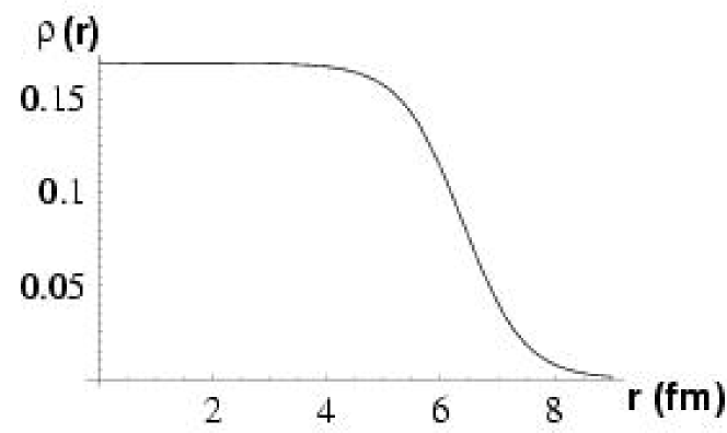
Figure 4.1: The Woods-Saxon Density profile for the Au nucleus.

With these parameters, we get a total number of nucleons in the Au nucleus of

$$\int_{0}^{\infty}\rho(r)\ 4\pi r^{2}\ dr=196.6\ \ .$$ (4.2)

It is also common in the literature to take a different value of $\rho_{0}$ such that the integral over the density is normalized to unity. We can then interpret $\rho(r)$ as the probability of finding a baryon in the volume element $d^{3}x=d^{2}bdz$ at the position $(\vec{b},z)$. With this convention, when calculating quantities such as the number of binary collisions, we see that there will be factors of $A$ every time this integral appears.

The next assumption is that the interaction probability is just given by the $pp$ cross section, neglecting effects like excitations and energy loss. At these energies, the $pp$ and the $p\bar{p}$ cross sections are very similar in value, and can therefore be used interchangeably. Unfortunately, there are no measurements of either cross section, $\sigma_{\mathrm{pp}}$ or $\sigma_{\mathrm{p\bar{p}}}$, at $\mbox{$\sqrt{s}$}=130\ \mbox{$\mathrm{GeV}$}$. The experiments UA5 [95] and UA1[96] at CERN-SPS have reported the $p\bar{p}$ cross section at $\mbox{$\sqrt{s}$}=900\ \mbox{$\mathrm{GeV}$}$. Although UA5 took data at $\mbox{$\sqrt{s}$}=200\ \mbox{$\mathrm{GeV}$}$, in Ref. [95] they only measure the ratio of the cross sections at the two different energies and use a parameterization given in  [97] (Eq. 4.3) to get a value for the total cross section. Then, based on the ratio $\sigma_{el}/\sigma_{tot}$ of elastic to total cross section, they obtain a value for $\sigma_{\mathrm{inel}}$.

$$\mbox{$\sigma_{\mathrm{p\bar{p}}}$}(\mbox{$\sqrt{s}$}) = C_{1}E^{-\nu_{1}}+C_{2}E^{-\nu_{2}}+C_{3}+C_{4}\ln^{2}(s)\$$ (4.3)

$$\mbox{$\sigma_{\mathrm{p\bar{p}}}$}(p) = A+Bp^{-n}+C\ln^{2}(p)+D\ln(p)\ .$$ (4.4)

For Eq. 4.3, the important part at energies above $\sim 100\ \mbox{$\mathrm{GeV}$}$ is the $\ln^{2}(s)$ term. The first two terms are used to describe the data at lower energies and the difference between $pp$ and $p\bar{p}$ collisions, $E$ is the beam energy. At $\sqrt{s}=130$ $\mathrm{GeV}$ and above, the $pp$ and $p\bar{p}$ cross sections are very similar. The parameterization found in the Particle Data Book  [39] is given in Eq. 4.4 in terms of the laboratory momentum $p$. They quote parameters for the total and for the inelastic cross section. The relevant numbers are found in Table  4.1. At the energy of the RHIC 2000 run, we obtain a value of $\mbox{$\sigma_{\mathrm{p\bar{p}}}$}(130\ \mbox{$\mathrm{GeV}$})\cong 40.35\ \mathrm{mb}$.

	$\sqrt{s}$ = 200 $\mathrm{GeV}$	$\sqrt{s}$ = 130 $\mathrm{GeV}$
$\sigma_{\mathrm{tot}}$	52.40 mb	49.26 mb
$\sigma_{\mathrm{el}}$	10.66 mb	8.91 mb
$\sigma_{\mathrm{inel}}$	41.74 mb	40.35 mb

Table 4.1: The $p\bar{p}$ total, elastic and inelastic cross sections obtained from the parameterization from the Particle Data Book  [39]. The errors on the values are on the order of 1%.

For head on collisions $b=0$, as we said before, in the hard sphere limit the number of participants will just be $2A$ where $A$ is the mass number of the nucleus. We need a prescription to calculate the overlap at any given impact parameter. This is given by the nuclear overlap integral, $\mathrm{T}_{\mathrm{AA}}$, which is a calculation of the overlap of the density profiles (in cylindrical coordinates, where the $z$ direction is the beam direction) of two specific nuclei at a given impact parameter $b$:

$$\mbox{$\mathrm{T}_{\mathrm{AA}}$}(b)=\int d^{2}s\ dz_{1}\ dz_{2}\ \rho_{1}(\vec{s},z_{1})\cdot\rho_{2}(\vec{s}-\vec{b},z_{2})$$ (4.5)

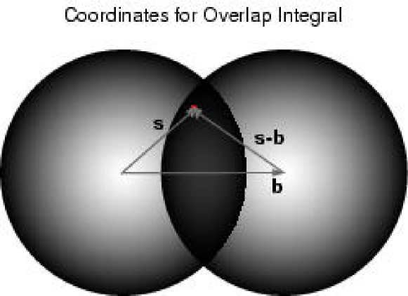
Figure 4.2: Schematic of the collision geometry for the calculation of the overlap integral $\mathrm{T}_{\mathrm{AA}}$, Eq. 4.5. The area of overlap is the “football” shaped region in the middle of the two spheres. The $z_{1}$ and $z_{2}$ coordinates are perpendicular to the plane of the paper.

We limit ourselves to the case of symmetric $AA$ collisions. The coordinate system is shown schematically in Fig. 4.2. For a given impact parameter, we calculate the product of the densities of each nucleus at a given point $\vec{s}$ and integrate over all space. We normalize the integral such that

$$\int\mbox{$\mathrm{T}_{\mathrm{AA}}$}(\vec{b})d^{2}b=1\ .$$ (4.6)

Since $d^{2}b$ is an element of area, $\mathrm{T}_{\mathrm{AA}}$ then has units of inverse area. With this definition, we can obtain the probability of having $n$ interactions at a given impact parameter

$$P(n,b)=\left(\begin{array}[]{c}A^{2}\\ n\end{array}\right)\left(\mbox{$\mathrm{T}_{\mathrm{AA}}$}(b)\mbox{$\sigma_{\mathrm{pp}}$}\right)^{n}\left(1-\mbox{$\mathrm{T}_{\mathrm{AA}}$}(b)\mbox{$\sigma_{\mathrm{pp}}$}\right)^{A^{2}-n}\ .$$ (4.7)

The first terms takes care of the combinations of choosing $n$ nucleons out of $A^{2}$, the second term is the probability of having exactly $n$ collisions and the third term is the probability of having exactly $A^{2}-n$ misses. The total hadronic cross section for $\mathrm{Au}+\mathrm{Au}$ collisions is then found to be:

$$\sigma_{\mathrm{AuAu}}=\int d^{2}b\ \left[1-(1-\mbox{$\mathrm{T}_{\mathrm{AA}}$}(b)\mbox{$\sigma_{\mathrm{pp}}$})^{A^{2}}\right]=7.2\ \mathrm{barn}$$ (4.8)

which can be read as 1 minus the probability of not having any collision ($n=0$) at a given impact parameter (i.e. the probability of having at least one interaction at each $b$) integrated over all impact parameters.

The mean number of binary collisions $\langle\mbox{$N_{\mathrm{coll}}$}\rangle$ and the mean number of participants $\langle\mbox{$N_{\mathrm{part}}$}\rangle$ are obtained from $\mathrm{T}_{\mathrm{AA}}$ at a given impact parameter as

$$\langle\mbox{$N_{\mathrm{coll}}$}\rangle(b) = \mbox{$\sigma_{\mathrm{pp}}$}\cdot A\cdot A\cdot\mbox{$\mathrm{T}_{\mathrm{AA}}$}(b)\$$

$$\langle\mbox{$N_{\mathrm{part}}$}\rangle(b) = 2A\int d^{2}s\ \mbox{$\mathrm{T}_{\mathrm{AA}}$}(\vec{s})\ \left\{1-\left(1-\mbox{$\mathrm{T}_{\mathrm{AA}}$}(\vec{s}-\vec{b})\mbox{$\sigma_{\mathrm{pp}}$}\right)^{A^{2}}\right\}\ .$$ (4.9)

Since the definition of the overlap integral takes care of counting interactions, it is not surprising that the number of binary collisions is simply proportional to $\mathrm{T}_{\mathrm{AA}}$. In the above definition of $N_{\mathrm{coll}}$, the factor $A^{2}$ comes from our choice of normalization.

 

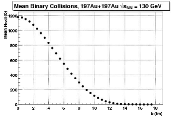
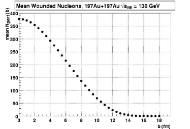
Figure 4.3: $\langle\mbox{$N_{\mathrm{part}}$}\ \rangle$ and $\langle\mbox{$N_{\mathrm{coll}}$}\ \rangle$ as a function of impact parameter.

Fig. 4.3 shows the resulting statistical relation between the impact parameter and $N_{\mathrm{coll}}$ ($N_{\mathrm{part}}$) in the left (right) panel. For large impact parameter, both $N_{\mathrm{part}}$ and $N_{\mathrm{coll}}$ are close to zero. For the most central collisions, $N_{\mathrm{part}}$ is found to be $\sim 394$ as expected. We see that the shapes are similar, although the overall scale is the different.

Indeed, Fig. 4.4 shows the statistical relation between $N_{\mathrm{part}}$ and $N_{\mathrm{coll}}$ as a function of impact parameter. The dotted curve corresponds to $\mbox{$N_{\mathrm{coll}}$}=(\mbox{$N_{\mathrm{part}}$}/2)^{4/3}$.

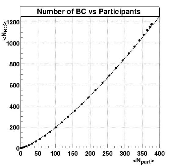
Figure 4.4: $\langle\mbox{$N_{\mathrm{coll}}$}\ \rangle$ correlated to $\langle\mbox{$N_{\mathrm{part}}$}\ \rangle$. The curve is the limit $\mbox{$N_{\mathrm{coll}}$}=(\mbox{$N_{\mathrm{part}}$}/2)^{4/3}$ .

The above definitions and relations are the basis of the geometrical model. We obtain a relationship between the $N_{\mathrm{part}}$ and $N_{\mathrm{coll}}$ as a function of impact parameter. These are still not directly measurable quantities in experiments. In a fixed target environment, one can try to estimate $N_{\mathrm{part}}$ by placing a hadron calorimeter to measure the forward-going energy, and thus approximately determine the spectator nucleons. In the RHIC environment, the closest we can get to such a scheme is to place calorimeters in the forward-backward regions, called zero degree calorimeters (ZDC’s) at RHIC, which detect the spectator neutrons (see Section  5.3). So there has to be another indirect step to model the particle production based on $N_{\mathrm{part}}$, $N_{\mathrm{coll}}$, and $\mathrm{T}_{\mathrm{AA}}$. There is not a unique way to do this. We will describe the “eikonal” approach to particle production given in Ref. [98] which was used already in the analysis of PHOBOS data [93].

We assume that each participant contributes to particle production, i.e. $\langle\mbox{$N_{h^{-}}$}(b)\rangle=q\langle\mbox{$N_{\mathrm{part}}$}(b)\rangle$ where $q$ is a scale factor. This approach has worked well at low energies, but at higher energies the hard processes contribute to particle production as well. Therefore, in [93], the assumption is that particle production scales as a linear combination of $N_{\mathrm{part}}$ and $N_{\mathrm{coll}}$. This model also attempts to incorporate the multiplicity measured in $pp$ collisions. The particle production is then given by:

$$\langle\mbox{$N_{h^{-}}$}(b)\rangle=q\cdot n_{\mathrm{pp}}\left(\sqrt{s}\right)\left((1-x)\cdot\frac{\left\langle\mbox{$N_{\mathrm{part}}$}(b)\right\rangle}{2}+x\cdot\left\langle\mbox{$N_{\mathrm{coll}}$}(b)\right\rangle\right)$$ (4.10)

The idea is that $x$ is a number between $0-1$ which gives the fraction of particle production that scales as $\sim\mbox{$N_{\mathrm{coll}}$}$. We also need the expected particle production per participant from $pp$ collisions. It is measured at 200 $\mathrm{GeV}$ [99, 96]. The number of charged particles in the collision per unit of pseudorapidity at mid-rapidity is reported in Ref. [96] to scale as

$$d\mathrm{N_{ch}}/d\eta(\mbox{$\sqrt{s}$})=-0.32+0.55\ln(\mbox{$\sqrt{s}$}/\mbox{$\mathrm{GeV}$})\ \ ,$$ (4.11)

which at 130 $\mathrm{GeV}$ yields $n_{\mathrm{pp}}=d\mbox{$N_{h^{-}}$}/d\eta|_{\eta=0}=2.36/2=1.18$ .

The next assumption is to pick the statistical distribution to model the fluctuations about the mean value. One can choose e.g. a Poisson distribution [100, 101] or a Gaussian distribution [93, 31]. We follow the Gaussian prescription here, we then require an additional parameter to get the variance for the Gaussian, which is taken as simply

$$\sigma_{g}^{2}=a\cdot q^{2}\cdot\langle\mbox{$N_{h^{-}}$}(b)\rangle\ .$$ (4.12)

The parameters of the model are thus $a$, $x$ and $q$.

We are finally in the position to calculate the multiplicity distribution, which is the actual experimental observable. This is done by convoluting the various Gaussian distributions obtained for each impact parameter, weighted by the appropriate interaction probability and integrating over all impact parameters:

$$\frac{d\sigma_{\mathrm{AuAu}}}{d\mbox{$N_{h^{-}}$}}(\mbox{$N_{h^{-}}$})=\int d^{2}b\ (1-P(0,b))\ \frac{1}{\sqrt{2\pi}\sigma_{g}}\ e^{\frac{N_{h^{-}}-\langle N_{h^{-}}(b)\rangle}{2\sigma_{g}^{2}}}$$ (4.13)

From such a picture, we expect roughly the following behaviour as a function of impact parameter. The cross section is largest for very peripheral collisions ($b\sim 12\ \mbox{$\mathrm{fm}$}$), dropping rapidly at first ($b\sim 12-10\ \mbox{$\mathrm{fm}$}$) and then falling more slowly in the region of mid-central collisions ($b\sim 8-4\ \mbox{$\mathrm{fm}$}$), eventually reaching a limit for the most central collisions ($b\lesssim 3\ \mbox{$\mathrm{fm}$}$). A schematic curve of the cross section as a function of multiplicity obtained from the hijing model [102, 103] is given in Figure 4.5. The multiplicity is the lowest ordinate axis. A related experimental observable is the transverse energy $E_{\perp}$ in the next axis. The percentage of the hadronic cross section is then given. The ordinate axes at the top of the figure are the non-measurable quantities which one can relate in the geometrical model to the multiplicity: $N_{\mathrm{part}}$ and the impact parameter $b$.

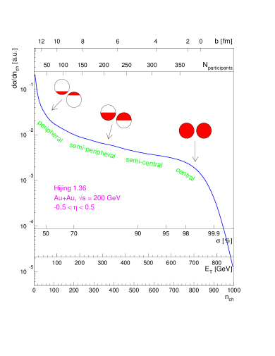
Figure 4.5: Schematic of a multiplicity distribution from the hijing model, showing the relationship between the shape of the distribution and the underlying collision geometry (see text). Figure prepared by T. Ullrich.

In this model, we obtain for the 5% most central $\mathrm{Au}+\mathrm{Au}$ events $\langle\mbox{$N_{\mathrm{part}}$}\rangle/2=$ 172 participant pairs [93] and $\langle\mbox{$N_{\mathrm{coll}}$}\rangle=$ 1050 using $\mbox{$\sigma_{\mathrm{inel}}$}\ =40.35$ mb.

4.2 Kinematic Variables: $p_{\perp}$, $m_{\perp}$, $y$ and $\eta$

The next observable after a simple measurement of the charged multiplicity is to look at the momentum distribution of particles. Particle spectra are often treated separately in the longitudinal and transverse directions.

For the transverse direction one normally employs the transverse momentum ($p_{\perp}$) or for identified particles the transverse mass

$$\mbox{$m_{\perp}$}=\sqrt{\mbox{$p_{\perp}$}^{2}+m^{2}}$$ (4.14)

where $m$ is the mass of the particle.

It is convenient to treat longitudinal momenta using the rapidity

$$y=\frac{1}{2}\ln\left(\frac{E+p_{z}}{E-p_{z}}\right)$$ (4.15)

where $E$ and $p_{z}$ are the energy and longitudinal momentum of the particle. The use of rapidity guarantees that the shape of the corresponding distribution is independent of the Lorentz frame. Under a Lorentz transformation from a reference system $R$ to a system $R^{\prime}$ moving with velocity $\beta_{z}$ with respect to $R$ in the longitudinal direction, the rapidity $y^{\prime}$ in the $R^{\prime}$ frame is related to $y$ in the $R$ frame only by an additive constant: $y^{\prime}=y-y_{\beta}$, where $y_{\beta}$ is the rapidity of the moving frame

$$y_{\beta}=\frac{1}{2}\ln\left(\frac{1+\beta_{z}}{1-\beta_{z}}\right)$$ (4.16)

For the incident energy of the Au beams at RHIC ($\gamma=70$), the initial rapidity of each Au beam is $y_{\mathrm{beam}}=\pm 4.94$, since the beams are symmetric. The rapidity of the centre-of-mass system, called mid-rapidity, is $y=0$; i.e. the centre-of-mass reference frame is the same as the laboratory frame for the collider geometry.

In the limit of a particle whose mass is much smaller than its momentum, the pseudorapidity variable $\eta$ is often used. It is defined as

$$y=\frac{1}{2}\ln\left(\frac{E+p_{z}}{E-p_{z}}\right)\approx\frac{1}{2}\ln\left(\frac{|\vec{p}|+p_{z}}{|\vec{p}|-p_{z}}\right)=\ln\left(\sqrt{\frac{1+\cos\theta}{1-\cos\theta}}\right)=-\ln\left(\tan\theta/2\right)\equiv\eta$$ (4.17)

For the case of negative hadron distributions, since no particle identification is performed, this is the variable of choice since one only needs to measure the angle $\theta$ of the detected particle relative to the beam axis (polar angle in spherical coordinates, also called dip angle in the helix parameterization commonly used in tracking). Sometimes in the literature $h^{-}$ distributions are also presented under the assumption that all particles are pions, e.g. [104, 105]. For the present work, the $h^{-}$ distributions are given in pseudorapidity since this is the actual measured observable, the identified $\pi$ distributions are given in rapidity.

The momentum distributions are usually presented in terms of the invariant cross-section

$$E\frac{d^{3}\sigma}{d^{3}p}=\frac{d^{3}\sigma}{d\phi dy\mbox{$p_{\perp}$}d\mbox{$p_{\perp}$}}=\frac{d^{2}\sigma}{2\pi dy\mbox{$p_{\perp}$}d\mbox{$p_{\perp}$}}=\frac{d^{2}\sigma}{2\pi dy\mbox{$m_{\perp}$}d\mbox{$m_{\perp}$}}$$ (4.18)

The double differential in Eq. 4.18 is obtained from integration over $\phi$, and the last equality follows from the definition of transverse mass, Eq. 4.14.

It is important to understand the difference in shape of the $y$ and $\eta$ distributions that arises simply from the change of variables. In particular, the Jacobian $\partial y/\partial\eta$ characterizes the difference between a distribution given as $d^{2}N/d\mbox{$p_{\perp}$}d\eta$ and one given as $d^{2}N/d\mbox{$p_{\perp}$}dy$. From the relation $p_{z}=\mbox{$m_{\perp}$}\sinh y=\mbox{$p_{\perp}$}\sinh\eta$, the Jacobian at fixed $p_{\perp}$ is

$$\frac{\partial y}{\partial\eta}=\frac{\mbox{$p_{\perp}$}\cosh\eta}{\mbox{$m_{\perp}$}\cosh y}=\frac{|\vec{p}|}{E}=\beta\ .$$ (4.19)

From this relation we again see that $\eta$ approaches $y$ for highly relativistic particles. The Jacobian in terms of the variables ($p_{\perp}$, $\eta$) and ($m_{\perp}$, y) is

$$\frac{\partial y}{\partial\eta}(\mbox{$m_{\perp}$},y) = \sqrt{1-\frac{m^{2}}{\mbox{$m_{\perp}$}^{2}\cosh^{2}y}}$$ (4.20)

$$\frac{\partial y}{\partial\eta}(\mbox{$p_{\perp}$},\eta) = \frac{(\mbox{$p_{\perp}$}/m)^{2}\cosh\eta}{\sqrt{(\mbox{$p_{\perp}$}/m)^{2}\cosh^{2}\eta+1}}\ .$$ (4.21)

We can then infer from Eq. 4.20 that in the region $y\approx 0$, there is a small depression in the pseudorapidity distribution $dN/d\eta$ relative to $dN/dy$. At high energy, where $dN/dy$ has a plateau shape, this leads to a small dip at mid-rapidity for $dN/d\eta$, with the $dN/d\eta$ yield being smaller by a factor of approximately $\sqrt{1-m^{2}/\langle\mbox{$m_{\perp}$}\rangle^{2}}$ relative to $dN/dy$.

4.3 Dynamics from the Kinematics

To understand the dynamics of relativistic heavy-ion collisions, it is essential to have information on certain basic aspects of the collision dynamics. The basic idea is that particle spectra act as kinematic probes. By analyzing the rapidity and transverse momentum distributions of the particles produced in the collision, one can study the energy density $\epsilon$, pressure $P$, and entropy density $s$ of the hadronic matter formed in the collision, as a function of temperature $T$ and baryochemical potential $\mu_{B}$ [106]. From Lattice QCD, the expectation is to observe a rapid rise in the effective number of degrees of freedom, expressed by the ratios $\epsilon/T^{4}$ or $s/T^{3}$ over a small range of temperatures [107]. Experimental observables which are thought to be related (e.g. in hydrodynamics) to $T$, $s$, and $\epsilon$ are the average transverse momentum $\langle p_{\perp}\rangle$, the hadron rapidity distribution $dN/dy$ [108, 109], and the transverse energy $d\mbox{$E_{\perp}$}/dy$, respectively [65]. (The average transverse momentum, or the related slope of the transverse momentum distributions, actually reflect not just the temperature in such models but also the transverse expansion of the system.) If there is a rapid change in the effective number of degrees of freedom due to deconfinement in the medium, the first hope was that one might see vestiges of this effect in a plot of $\langle p_{\perp}\rangle$ as a function of $dN/dy$, which would be expected to show a rise, then a characteristic saturation of $\langle p_{\perp}\rangle$ while the mixed phase persists and then a second rise when the underlying matter undergoes a structural change to its coloured constituents[65]. This simple picture however has several caveats. We discuss here a few of them. We already stated that it is much too naïve to identify $\langle p_{\perp}\rangle$ or the inverse slope parameter of a transverse momentum spectrum directly with the temperature of the system. It is also simplistic to assume that the exponential shape arises in an identical manner as that of a Boltzmann gas that reaches thermal equilibrium through a series of internal collisions of the particles in the system. Statistical thermal models [110] have even been applied to $\mathrm{e}^{+}\mathrm{e}^{-}$ collisions in fits to hadronic particle spectra [111]. The observed spectra for $\mathrm{e}^{+}\mathrm{e}^{-}$ collisions certainly do not come about because of a hadronic rescattering of the final state particles, but are a the result of a sampling of the available phase space, i.e. the particles are already born into equilibrium [112]. Furthermore, if the system formed in $AA$ reaction does in fact thermalize through collisions, the final state particles observed in the experiments, and in particular the momentum spectra, will only reflect the coolest phase of the evolution of the system. Stated another way, if thermalization occurs the effective temperature extracted from the spectrum (even if we assume we can take care additional collective effects such as flow which modify the $p_{\perp}$ distributions) will probably not carry information of the hot initial phase, smearing any structure in a $\langle p_{\perp}\rangle$ vs. $dN/dy$ plot. In addition, a visible flat structure in the ‘$T$ vs. $\epsilon$’ diagram necessitates a significant duration of a mixed phase, an effect that probably requires the presence of a strong first-order phase transition. However, lattice simulations currently favour a more smooth cross over, perhaps a second order transition. In this respect, critical phenomena in the form of increased event-by-event fluctuations are possibly a more robust observable with respect to the existence of a phase transition. Even in this case, fluctuation studies would necessitate probing the region near a possible critical point in the $T-\mu_{B}$ phase diagram, and current efforts to shed light as to the presence and location of a critical point indicate it is in the large $\mu_{B}$ region [113].

Rapidity and transverse momentum distribution also allow us to address properties of the particle emitting source. The degree to which the incoming nuclei are stopped by the collision is reflected in the rapidity distributions of produced particles as a shift with respect to beam rapidity. At sufficiently high energies for example, a picture due to Bjorken [59], assumes that the mid-rapidity region should undergo an idealized hydrodynamic longitudinal expansion. The charged particles found at mid-rapidity would be mainly produced particles, the energy of the incoming nuclei would be so great that the collision among the nucleons would be insufficient to stop the nuclei, so the incoming nuclei would essentially go right through each other. The incoming baryons are then found very close to their initial rapidity. More importantly, the rapid longitudinal expansion would have as a result that the rapidity distribution of produced particles should be flat around mid-rapidity.

This contrasts the picture found at AGS energies, where a significant amount of stopping is observed and the mid-rapidity region is net-baryon rich. This is reflected in the rapidity distribution of charged particles which is peaked at mid-rapidity, as are the net-proton distributions ($p-\mbox{$\bar{p}$}$). Full stopping as in the model of Landau [108] is expected then to work at low energies, and the rapidity distribution of produced particles at mid-rapidity is found to more closely follow a Gaussian shape [114, 115, 116]. Since the observed width of the distribution is significantly narrower than that observed for lighter systems, this has been understood as evidence for strong baryon stopping.

From the rapidity distributions, we can therefore obtain information for example, as to whether the source is spherically symmetric or elongated, whether it is static or expanding, and the degree of longitudinal and transverse expansion. The momentum distributions, when paired with elliptic and transverse flow studies, can also test if there is significant collective behaviour in the system and approach the question of whether the system reaches thermal equilibrium. Experimentally, one can test the hypothesis of boost invariance by measuring $\eta$ and $y$ distributions. If the system is boost invariant to a certain extent and $dN/dy$ is flat as a function of rapidity in some phase space range, the $h^{-}$ pseudorapidity distribution should be well approximated by Eq. 4.21. The rapidity distribution of identified particles should simply be constant as a function of $y$. The slope parameter of $\pi$ distributions have also been found to show a significant rapidity dependence at lower energies [114, 115, 116, 117]. We can measure the rapidity dependence of the $\pi$ spectra at RHIC and further test the hypothesis of boost invariance. These are of course not sufficient conditions to establish boost invariance, but they are necessary in case it does hold.

4.4 Overview of Transverse Momentum Spectra

The transverse momentum spectra possess many interesting features in $AA$ collisions. The use of the transverse mass $m_{\perp}$ is sometimes preferred because experimentally the cross-section $(1/\mbox{$p_{\perp}$})(d\sigma/d\mbox{$p_{\perp}$})$ of a given particle species is better described by an exponential in $m_{\perp}$ rather than in $p_{\perp}$ [118]. There are contributions to the spectrum that come from the various physics processes of interest. In order to extract correct information about the collision, it is necessary to take these into account. Even now, our understanding of all the features of the spectra is incomplete. A brief overview of the main features of the $p_{\perp}$ distributions will be discussed.

A general feature emerging from measurements of transverse momentum distributions in central collisions of heavy nuclei is that the invariant distributions $d^{2}N/\mbox{$m_{\perp}$}d\mbox{$m_{\perp}$}dy$ are approximately exponential, i.e. $d^{2}N/\mbox{$m_{\perp}$}d\mbox{$m_{\perp}$}dy\propto\exp(-\mbox{$m_{\perp}$}/T)$. One approach to analyze the $p_{\perp}$ distributions has been to treating the system as a hadronic gas, and in particular to use the measured $\langle p_{\perp}\rangle$ to estimate the freeze out temperature $T$ of the gas and its transverse flow velocity $\mathrm{\beta_{\perp}^{flow}}$. These also have inverse slope constants $T$ increasing linearly with the mass of the particle under study. This has been interpreted as evidence for collective transverse flow: since $\mbox{$p_{\perp}$}=m\gamma\beta_{\perp}$, if there is a common flow velocity $\mathrm{\beta_{\perp}^{flow}}$ superimposed on the random thermal motion of particles $\beta_{\perp}^{\mathrm{thermal}}$, the slope constant $T$, which is proportional to $\langle p_{\perp}\rangle$ increases linearly with $m$. It is important to note, however, that in these models, $T$ and $\mathrm{\beta_{\perp}^{flow}}$ are coupled: a higher $T$ can compensate for a lower $\mathrm{\beta_{\perp}^{flow}}$ and vice versa. This approach relies only on the analysis of $p_{\perp}$ spectra. It must also be noted that in a plot of $T$ vs. mass, it is difficult to make meaningful comparisons of slope parameters when they are obtained from different phase space regions, and there is the danger of obtaining a very different slope simply by fitting in a different part of the $p_{\perp}$ spectrum. Therefore, rather than concentrating on the slope parameters, more realistic models incorporate additional observables such as two-particle correlation data [119] and attempt to describe both the observed $p_{\perp}$ distributions and the observed correlations to obtain $T$ and $\mathrm{\beta_{\perp}^{flow}}$.

The slope of the $p_{\perp}$ distribution is also seen to increase in going from $pp$ to $AA$. The spectrum of the pion, due to its low mass, is not as affected as the spectra of heavier particles by a given collective flow velocity. Thus, the pions are good probes for studying thermal properties at freeze-out. These features of spectra can be measured at RHIC energies, and the linear scaling of spectra with the mass of the particle checked. The scaling could very well be reduced given that RHIC energies are a significant leap with respect to SPS energies, and the collision process can occur in a short enough time scale such that particles involved might not have time to develop a significant flow velocity. On the other hand, an increase in the radial flow (and also of the elliptic flow $v_{2}$) would signal an significant amount of collective behaviour. Uncertainties remain, and they will only be clarified once we measure spectra and compare them with the various scenarios: from superposition of $pp$ collisions governed by measured hadronic cross sections; to relativistic microscopic models based on string formation and string fragmentation (where a string is represented by the color flux tube from a quark and a diquark. In longitudinal exchange string formation, the excitation of the string originates from a stretching of the original partons in the hadron caused by a large longitudinal momentum exchange from the hadronic collision. hijing, fritiof and rqmd use this scheme.); to hydrodynamics, which can be thought of the limit where the mean free path of the constituents is zero and the system is a fluid.

It is also known that there are significant deviations from a purely exponential spectrum, both at low and high-$p_{\perp}$ [120]. The high-$p_{\perp}$ region (at SPS, $\mbox{$p_{\perp}$}\gtrsim 1.5\ \mbox{$\mathrm{GeV/}c$}$) shows an enhancement present already in $pA$ collisions known as the Cronin effect [121]. This enhancement shows a strong dependence on both target and projectile mass, and a weak rapidity and $\sqrt{s}$ dependence. It is thought to be partly due to multiple low-momentum scattering at the partonic level inside nuclear matter. Perturbative QCD calculations for $pA$ have been done [122] and agree reasonably with data. However, a complete quantitative understanding of this effect has not yet been achieved. The CERES collaboration measured spectra in $pA$ collisions, found a similar effect when comparing to $pp$, and reached similar conclusions. Their S+Au data indicated that the onset of this enhancement occurred at lower $p_{\perp}$ and that the overall enhancement was larger. This was taken as evidence that in $AA$ collisions, there is an increased number of scattering processes per parton compared to $pA$ collisions, leading to increased thermalization of the collision system. In addition, the shape of the high $p_{\perp}$ spectrum was very close to being exponential. These two observations suggested that a large degree of thermalization is reached very early for central S+Au collisions at $\mbox{$\sqrt{s_{{}_{\mathrm{NN}}}}$}\sim 20\ \mbox{$\mathrm{GeV}$}$.

The low-$p_{\perp}$ region shows an enhancement as well. This enhancement, however, shows different systematic behaviour than the high-$p_{\perp}$ excess. The underlying physics that give rise to this enhancement are different than in the high-$p_{\perp}$ region. In fixed target experiments, the low-$p_{\perp}$ enhancement was observed to have a strong target dependence but weak projectile dependence, as well as a strong rapidity dependence. These effects are not yet completely understood. There have been several attempts at explaining the enhancement (at least qualitatively). Resonance decays are thought to contribute significantly in this region [123, 124], and their contribution to the low-$p_{\perp}$ enhancement would also be consitent with the observed strong dependence on target and rapidity. Produced particles can also rescatter in the target nucleus, and the ensuing cascade would yield additional soft pions and resonances. In addition, at the lowest $p_{\perp}$ one should expect that the treatment of a radiating gas based on Boltzmann statistics must break down, and one should really use either Bose-Einstein or Fermi-Dirac distributions to fit the data. For pions, a Bose-Einstein fit will give a natural low-$p_{\perp}$ enhancement compared to a Boltzmann fit to the spectrum. Other processes can also contribute to the low-$p_{\perp}$ region, but our understanding of the enhancement is by no means complete at this point. Studying this region at RHIC energies will certainly help to shed light on the subject.

To fully understand the non-hadronic effects that may arise in an $AA$ collision, studying the particle distributions, in order to obtain basic information about the collision dynamics, is a necessary step. Several approaches have been proposed to describe the observed transverse momentum spectra, and to obtain different types of information from them. In the absence of any collective behaviour, the spectra should be a simple geometrical superposition of nucleon-nucleon scatterings. A deviation of the particle distributions observed in $AA$ collisions from those observed in $pp$ or $p\bar{p}$ collisions is already strong evidence for some form of collective behaviour. We discuss two models that have almost diametrically opposite assumptions.

In hydrodynamic models, the colliding system is treated as a fluid, and can be thought of as the limit of zero mean free path among the constituent partons. The transverse momentum distributions are obtained from a transverse flow velocity profile of the component particles of the fluid. The profile will depend in general on the initial conditions (centrality, initial energy density) as well as the underlying equation of state (including or not a phase transition) as a function of time. This models typically yield the strongest signals for collective effects such as elliptic flow an longitudinal expansion. They should work best at low transverse momentum, and their signals can be tested for example by measuring the centrality dependence of the elliptic flow signal.

In partonic cascade models, the energy deposition in the collision is broken up into scattering of the constituent partons of the colliding nuclei. They rely on the framework of perturbative QCD, following the perturbative interactions among partons until they reach thermal equilibrium. These models predict a very rapid thermalization, mainly due to radiative energy degradation, which yields a transverse momentum distribution that is exponential to a high degree. In all these theoretical models, the shape of the particle distribution yields information to the underlying collision dynamics. Since they rely on perturbative calculations, they should work best for hard processes such as jets and high-$p_{\perp}$ momentum spectra.

There are, of course, other observables that need to be studied to provide further insight into the full picture of the reaction process. These include studies of strangeness production, HBT correlation analyses, and fluctuations of observables on an event-by-event basis. These and other questions are also being addressed in STAR. The particle distributions are, however, a very basic building block of the collision picture, and one of the first that can and has to be addressed in the initial stage of the experiment.

In previous heavy-ion experiments at lower energies, the study of the particle spectra has helped to provide guidance into interesting aspects of the collision dynamics, and has also provided a means to compare results with model calculations [125]. The usefulness of studies with particle spectra is best illustrated with a few examples.

4.5 Previous Studies Using $m_{\perp}$ Spectra

At the BNL-AGS, E877 [114] measured hadron spectra from Au+Au collisions at 10.8 $\mathrm{GeV/}c$ per nucleon. They measured proton and pion $m_{\perp}$ distributions as a function of $y$ and performed exponential fits to extract inverse slope constants from the spectra. For both pions and protons, the spectra showed deviations from the simple exponential, e.g. an excess for pions was observed at $\mbox{$m_{\perp}$}-\mbox{$\mathrm{m_{\pi}}$}<0.2\ \mbox{$\mathrm{GeV/}c^{2}$}$, with the excess increasing systematically as one approached mid-rapidity. They compared the $\mathrm{Au}+\mathrm{Au}$ inverse slope constants extracted from the measured $m_{\perp}$ spectra with a lighter system, Si+Al. The slope parameter in the $\mathrm{Au}+\mathrm{Au}$ case systematically increased when going from the fragmentation region to central rapidities. The data indicated that the maximum the observed slope parameter would be reached around mid-rapidity (e.g. the measured inverse slopes for protons at $y/y_{\mathrm{beam}}=0.7$ were $\mbox{$T_{\mathrm{eff}}$}\sim 150\ \mbox{$\mathrm{MeV}$}$ for Si+Al and $\mbox{$T_{\mathrm{eff}}$}\sim 250\ \mbox{$\mathrm{MeV}$}$ for $\mathrm{Au}+\mathrm{Au}$). This could be interpreted as being due to a larger collective transverse flow component in Au+Au compared to that of Si+Al. The proton rapidity distribution was also measured for both systems, being much narrower in Au+Au. This provided information as to the degree of stopping in the collision. The greater stopping observed in the Au+Au system was interpreted as being a consequence of the smaller surface to volume ratio as well as the increased average number of rescatterings. E877 also measured pion spectra in Au+Au collisions. The rapidity distributions were well matched by calculations from RQMD, an event generator based on hadronic rescattering using a mean field approximation [126]. The $m_{\perp}$ spectra, and specifically the low-$m_{\perp}$ region ($\mbox{$m_{\perp}$}-\mbox{$\mathrm{m_{\pi}}$}<0.2\ \mbox{$\mathrm{GeV/}c^{2}$}$) showed an enhancement above the pure exponential. In addition, the deviations were seen to be systematically larger for $\pi^{-}$ than for $\pi^{+}$. This asymmetry was also observed to systematically decrease as a function of rapidity, an effect seen also by the E866 collaboration[127]. This was interpreted as due to the different Coulomb potentials seen by the different charge types at freeze-out. (Coulomb interactions are also relevant to the interpretation of particle correlation studies.) The study of the influence of the Coulomb effect on the shape of the particle spectra provided E877 with a different approach to determine the spacetime particle distribution at freeze-out.

At the CERN-SPS, several experiments have measured charged hadron spectra. NA49 [119] in central Pb+Pb collisions measured $m_{\perp}$ spectra of charged pions. They also measured two-particle correlation functions to deduce parameters from the collision dynamics. As mentioned earlier, in a typical fit to an $m_{\perp}$ distribution, one can trade lower values of $\mathrm{\beta_{\perp}^{flow}}$ for higher values of $T$. NA49 applied a model including longitudinal and transverse expansion [128, 129] using both the $h^{-}$ and deuteron transverse momentum spectra as well as results from two-particle correlations. They were thus able to constrain the region for the freeze-out temperature $T$ and the transverse flow velocity $\mathrm{\beta_{\perp}^{flow}}$ to $T=120\pm 12\ \mbox{$\mathrm{MeV}$}$ and $\mbox{$\mathrm{\beta_{\perp}^{flow}}$}=0.55\pm 0.12$ [119]. Comparison of the charged hadron spectra to predictions of a simple hydrodynamical model[125], yields similar values for $T$ and $\mathrm{\beta_{\perp}^{flow}}$ assuming a quark-gluon plasma first order phase transition at a temperature $\mbox{$T_{c}$}\sim 160\ \mbox{$\mathrm{MeV}$}\$ (where $T_{c}$ was fixed by the lattice results then available). Under these assumptions, the data favor a relatively low kinetic freeze-out temperature compared to the critical temperature, consistent with the picture from Fig. 3.1.

CERES [104] in Pb+Au collisions measured $m_{\perp}$ spectra of identified pions and negative hadrons as well as ‘net proton’ ($h^{+}-h^{-}$) spectra. Fourier analysis studies of the azimuthal charged particle distribution with respect to the reaction plane were performed. The amplitude of the first harmonic, $v_{1}$, is associated with directed flow. The second harmonic coefficient, $v_{2}$, is called elliptic flow. The pseudorapidity dependence of these two coefficients was studied as a function of centrality, giving strong evidence for collective behaviour in these collisions. In addition, a comparison of the ‘net proton’ spectrum from CERES with random-walk models allowed one to conclude that these models were not suitable to describe the flow-like features observed in the transverse momentum spectra.

For many of these measurements, a large acceptance detector such as STAR is ideal. We now proceed to discuss the STAR experimental setup for the RHIC summer 2000 run.

Chapter 5 The STAR Experiment

The main thrust of the STAR detector is dedicated to the heavy ion collision programme. It must cope with the large event multiplicities associated with central heavy ion collisions, and with the large interaction rates expected at RHIC. The collider was designed to deliver a luminosity of $\mathcal{L}=2\times 10^{26}$ cm^-2 s^-1 for $\mathrm{Au}+\mathrm{Au}$ collisions at $\sqrt{s_{{}_{\mathrm{NN}}}}$ = 200 $\mathrm{GeV}$. STAR is also designed with several other physics programmes in mind. It has the capability to measure the products from ultra-peripheral heavy ion collisions in order to study coherent photon and pomeron interactions from the intense electric fields originated by the Au nuclei [130, 131]. There will also be $pp$ and $pA$ collisions at RHIC to obtain information on nuclear parton distribution functions and for heavy ion reference data. In addition, there is a strong programme of polarized $pp$ collisions starting in 2001 which aims to measure the contributions from the gluon (and from sea-quarks) to the total spin of the proton [132].

This presents a challenge, since STAR has to deal with a wide dynamic range in several areas. For heavy ion collisions, the number of particles to be reconstructed in the detector vary from less than 10 for peripheral $\mathrm{Au}+\mathrm{Au}$ events to as many as $\sim 1000$ for central collisions. The interaction rates are large: RHIC reached its goal for the first year of delivering 10% of the design luminosity. The collider is designed to operate with 60 bunches in each ring. The time between beam crossings assuming all 60 bunches are filled and taking into account the perimeter of the RHIC rings (3.83 Km) is $\simeq 0.21\ \mu$s.

The rates will be even larger for polarized $pp$ collisions ($2\times 10^{32}$ cm^-2 s^-2). Coupled to the large amount of information recorded in the TPC, STAR must handle a large rate to tape (20 Mb/s for the 2000 run, double the number for 2001). As this would be the first year of RHIC operations, this also presented an opportunity: a wide range of available energies would now fall under experimental scrutiny. The excitement of getting the first glimpse at the data taken by the experiments was felt throughout the community, and was well matched with the struggle to understand the systematics of the different detector systems.

The STAR experimental setup for the year 2000 run centered around charged particle tracking using a large acceptance Time Projection Chamber (TPC). The trigger detectors were a pair of hadron calorimeters placed in the very forward/backward direction and a barrel of scintillator slats surrounding the TPC. In addition, a Ring Imaging Čerenkov detector (RICH) placed at mid-rapidity provides particle identification for high momentum particles. The STAR experiment with the main detector subsystems which are in place for year 2001 data is illustrated in Fig. 5.1. In place for the year 2000 were the Central Trigger Barrel, the Zero Degree Calorimeters, the magnet, the TPC and the RICH (the ZDC and the RICH are not shown, as the ZDC is far from the detector center and the RICH is located under the TPC and obstructed from view in the figure).

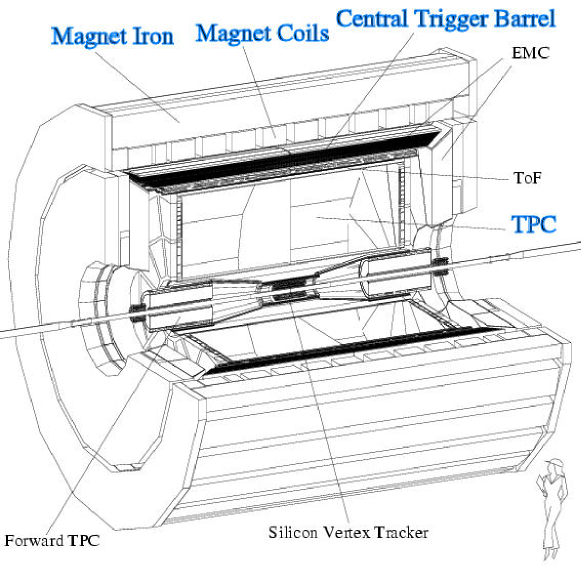
Figure 5.1: The STAR Detector

5.1 Magnet

Of critical importance to the experiment, the STAR magnet is designed to provide a very uniform field parallel to the beam direction. It is constructed as a large solenoid which must house the main subsystems of STAR: the TPC, central trigger barrel, and RICH. The strength of the field can be tuned from 0 up to 0.5 T, the strength used for the 2000 run was set to $B_{z}=0.25$ T. Having a uniform field is desirable for it greatly simplifies the track model used in the pattern recognition in the offline analysis: all charged tracks follow a helical trajectory to first order. The field uniformity at full strength was better than $\pm 40$ Gauss in the radial direction and $\pm 1$ Gauss in the azimuthal direction. The magnetic field was mapped before TPC installation to a precision of 1-2 Gauss for all components of the field. This allows a calculation of the distortion effects on tracks due to field inhomogeneities to a precision of $\sim 200-300\ \mbox{$\mu\mathrm{m}$}$.

5.2 STAR Time Projection Chamber

The main tracking detector for STAR is a large Time Projection Chamber (TPC) with complete azimuthal acceptance. With the magnetic field of 0.25 T, the $p_{\perp}$ acceptance for charged particles starts is $\mbox{$p_{\perp}$}\geq 50\ \mbox{$\mathrm{MeV/}c$}$. Particle identification is achieved by measuring the ionization energy loss $\frac{dE}{dx}$, applying topological cuts, or reconstructing invariant masses of pairs of particles.

The TPC tracking volume is 4 meters in diameter and 4.2 meters long. It is shown schematically in Fig. 5.2.

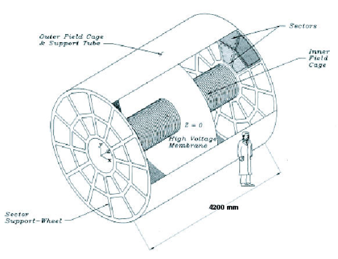
Figure 5.2: Schematic view of the STAR Time Projection Chamber.

The inner radius of the tracking volume starts at 50 cm. The outer radius subtends a pseudorapidity interval of $\pm 1$ unit and the corresponding range for the inner radius is $\pm 2$ units. Thus, the useful tracking volume extends out to $\sim\pm 1.5$ units due to a requirement of having at least 10 padrow hits in order to reasonably reconstruct a track. For the analysis discussed in this work, we focused on the tracks crossing the entire tracking volume to reduce systematic effects from variations in acceptance. The tracking volume is split in two along the beam direction as shown in Fig. 5.2. The two halves are divided by a high voltage cathode located at the center of the TPC (z=0), labelled “high voltage membrane” in the figure, but called simply the central membrane among the collaboration. The TPC gas is a mixture of 90% Ar and 10% methane (P10). Part of the considerations to choose P10 were that the gas should not attenuate the drifting electrons and it must be pure enough to prevent other modes of electron loss due to attachment on oxygen and water molecules. This means that the oxygen concentrations should be kept below a hundred parts per million. These stringent standards have already been met by P10 in the past [133].

The path of a track crossing 150 cm of this mixture is equivalent to 1.17% of a radiation length. The tracking volume is surrounded by an electrostatic field cage which is built with 11.5 mm wide rings to divide the voltage evenly, achieving a uniform decrease from -31 kV at the central membrane to 0 V at the ground wires. Secondary electrons produced by charged tracks ionizing the gas will drift in the $E$ field away from the central membrane to the nearest endcap. The field cages are very thin: 0.62% radiation lengths for the inner field cage and 1.26% radiation lengths for the outer field cage. The drift velocity of the electrons was measured to be 5.44 $\pm$ 0.01 cm/$\mu$s, where the 0.01 here denotes the size of variations over a period of several days. For a given run, the drift velocity was monitored to a precision of $\sim 0.001$ cm/$\mu$s. For such a large TPC, the gas and magnetic field strength are also important to maintain the diffusion of the drifting electrons to acceptable levels. The transverse diffusion in P10 at full field (0.5 T) is $\sigma_{T}\approx$230 $\mu\mathrm{m}$/ $\sqrt{\mathrm{cm}}$ or equal to a width of 3.4 mm after the drift; and this sets the scale for the dimensions of the pads under the anode wires, described below. Similarly, the longitudinal diffusion is $\sigma_{L}\approx 360\ \mbox{$\mu\mathrm{m}$}/\sqrt{\mathrm{cm}}$. For a cluster that drifts the full length of the TPC, this translates into a longitudinal width $\sigma$ = 0.52 cm , corresponding to a drift time of $\sim$95 ns. This determines the electronic sampling rate of 10 MHz, or every 100 ns, in order for a simple three point tracking and clustering algorithms to work well.

The drifting electrons are amplified by a grid of wires on each end of the TPC and the pulses are read out on small pads placed behind the anode wires. Each endcap of the TPC is segmented in the azimuthal direction like the face of a clock into 12 pad arrays, called sectors. This is illustrated Fig. 5.3 which shows the end view of the TPC.

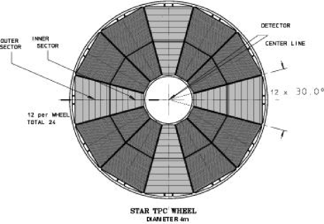
Figure 5.3: End view of the STAR TPC, where we see the 12 sectors covering the full azimuthal range.

The beam ($z$ axis) goes through the center of the TPC, perpendicular to the page in this view.

The geometry of one of the sectors is shown in Fig. 5.4.

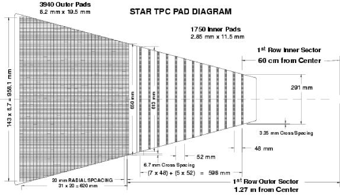
Figure 5.4: Schematic of a full TPC sector with pads. The first 13 rows comprise the inner sector, and rows 14-45 are the outer sector pads.

Each sector is divided into two parts, an inner and an outer sector. The inner sector has 1,750 pads, each pad measures 11.5 mm in the radial direction and 2.85 mm in the tangential direction. The inner sector pads were made as small as practical in order to provide closer space points for an improved two-track resolution. The size is limited by the diffusion limit of the TPC. They are grouped into 13 pad rows located between 60 cm and 116 cm from the beam line, measured from the center of the padrow. The outer sector has 3,940 pads, and the corresponding dimensions are 19.5 mm (radial) and 6.2 mm (tangential). The outer sectors spans 32 pad rows between 127.2 cm and 189.2 cm radius. The large outer sector pads completely cover the area under the anode wires. The gap between adjacent pads in the same row is 0.5 mm for both the inner and the outer sector.

Figure 5.5: Side view of the inner and outer sector of the STAR TPC showing the wire geometry. All distances are shown in mm.

The wire geometry is depicted in Fig. 5.5 where we see a cross-sectional view of the wire layers and of the pad plane. There are 3 layers of wires terminating each side of the chamber. The first layer is the gating grid. The wires of the gating grid are arranged to terminate the field cage voltage and it is therefore used to prevent ionization from reaching the anode wires of the chamber when no trigger is detected. The gating grid also helps minimize the space charge effects due to the presence of positive ions with very low mobility. The second layer is the ground plane, 6 mm below the gating grid, which captures the ions from the amplification region. The third layer is the anode plane, 2 mm (4 mm) below the ground plane in the inner (outer) sector, where gas amplification is achieved. The induced signal is picked up on the pad plane located 2 mm (4 mm) under the anode wires in the inner (outer) sector. In order to keep the signal to noise ratio constant at 20:1 for both pad sizes, the anode voltages were set to achieve a gain of 1100 on the outer sector and 3000 on the inner sector.

Combining the inner and outer sector, there are a total of 5690 pads per sector which corresponds to a total of 136,560 channels for all 24 TPC sectors. The signal measured on the pads is amplified using custom CMOS integrated circuits  [134]. These consist of a pre-amplifier and shaper circuit followed by a Switched Capacitor Array (SCA) and a 10 bit Analog-to-Digital Converter (ADC). These are responsible for sampling the arrival of the electrons into at most 512 time bins and to digitize the signal on the pads. Including the segmentation in the time (drift) direction, the TPC can be thought of as a large 70 megapixel 3D digital camera. The position of the particle along the drift direction is then reconstructed by converting from time bin to position by knowing the drift velocity. The position resolution along the drift direction for the summer 2000 run was on the order of 500 $\mu\mathrm{m}$. The front-end electronics are bundled into groups of 16, with the pre-amp, shaper and buffer in one chip, and the SCA and ADC in another chip. Two groups of 16 channels make up each front-end board, making a total of 32 channels and 4 chips per board. The data are sent to the Data Acquisition system (DAQ) over optical fibers. The full TPC DAQ rate is designed to be read out once per second for central $\mathrm{Au}+\mathrm{Au}$ collisions, which produces a rate to tape of $\sim$20 Mbytes/s.

For a more complete description of the STAR TPC see  [135, 136]. More detail on the TPC operation will be presented in Chapter 7 where we describe the physical processes of the TPC that were simulated for Monte Carlo studies. For more information on drift chambers, the standard reference is [133].

5.3 Trigger Detectors

The trigger detectors are an array of scintillator slats (CTB) arranged in a barrel at the outer diameter of the TPC; and two hadronic calorimeters (ZDCs) at $\pm 18$ m from the detector center and at close to zero degrees relative to the beam axis. The ZDC units subtend an angle of $\sim 2.5$ mrad from the interaction point. The calorimeters are designed to measure neutrons emitted from nuclear fragments of the spectator matter, i.e. matter that did not interact in the collision. In contrast to fixed target experiments, where one can measure all spectator nucleons in the forward direction, at RHIC the proton trajectories will be deviated by the dipole magnets in the beam line. The same dipole magnets that are used to steer the beam head on at each interaction region will bend the charged fragments away from the ZDCs. Protons of the same momentum as the Au ions are actually deviated by a larger angle, since they have a larger charge-to-mass ratio. Ergo the ZDC signal is produced by neutrons. Nevertheless, they still provide possibly the best determination of the collision centrality at RHIC, and are used for triggering (along with some other observable based on multiplicity) in all four experiments. This can serve as a standard for comparisons among the different results.

During the Summer 2000 run, RHIC delivered collisions between Au nuclei at $\mbox{$\sqrt{s_{{}_{\mathrm{NN}}}}$}\ =130\ \mbox{$\mathrm{GeV}$}$. The data presented here are from a minimum-bias sample, triggered by a coincidence of signals above threshold in both ZDCs with the RHIC beam crossing. The ZDC threshold was set to ensure efficient detection of single spectator neutrons. The efficiency of the ZDC coincidence trigger for central events was measured using a high-threshold CTB trigger. The trigger efficiency was found to be above 99% for the entire range of multiplicities reported in this study. The CTB was used to trigger on central events, as the signal is correlated to the multiplicity at mid-rapidity. The threshold for the central trigger using the CTB was set to obtain the events with the 15% highest CTB signals. The maximum luminosity achieved in 2000 was $\sim 10\%$ of the design luminosity. This translates into a hadronic interaction rate of $R=\mbox{$\sigma_{\mathrm{AuAu}}$}\times\mathcal{L}\simeq(7.2\times 10^{3}\ \mathrm{mb})\times(0.02\ \mathrm{mb}^{-1}\mathrm{s}^{-1})=144\ \mathrm{Hz}$. For higher luminosities, the trigger will certainly play an important role.

5.4 RICH

A Ring Imaging Čerenkov detector (RICH) was placed outside the CTB. The RICH covers a smaller area, 1 m $\times$ 1 m and is designed to provide high precision velocity measurements for enhanced particle identification at high momentum. The momentum information is provided by the TPC. One then uses this information to search for Čerenkov photons in 3 different annulus regions. For tracks with a perpendicular trajectory to the RICH, the regions will be circles of different radii depending on the particle’s velocity, which for a known momentum uniquely determines the mass of the particle. In the presence of the magnetic field, the trajectory of the tracks will not be normal to the RICH detector, so the Čerenkov photons will not be found in a circular region, but one can still determine the bounds of the search region analytically. The RICH detector is not used in this analysis, but it is the subject of another STAR thesis [137]. For more information on the RICH detector see [138].

The detector upgrades planned for the upcoming STAR runs include a Silicon Vertex Tracker (SVT), an Electromagnetic Calorimeter to cover the barrel at mid-rapidity around the TPC and one of the endcaps, a Time-of-Flight patch replacing one of the CTB slats, two Forward TPCs ($2.5\leq|\eta|\leq 4$) and additional Beam-Beam Counters for the trigger system. The hermeticity of the STAR detector when all the components are installed is shown in Figure 5.6.

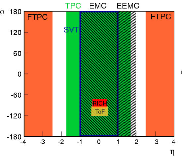
Figure 5.6: Hermeticity of STAR, including all detectors. Note that the RICH occupies real estate that will used for the full barrel EMC when completed, so this plot only illustrates their coverage.

Chapter 6 Reconstruction and Calibration

We discuss here the STAR offline reconstruction and analysis software relevant for the results presented in this work. The offline simulation and reconstruction software is a major component of the experiments, as we rely on it to reconstruct the collision event to a sufficient extent that the physics goals and the physics capabilities of the sub-detectors can be realized, to sufficiently evaluate and visualize the results to determine their adequacy and correctness, and to generate acceptance and reconstruction efficiency tables, among other things. The offline software includes all major sub-detectors. We will focus on the reconstruction done in the TPC, as this was the main detector used in STAR during the first run and is the relevant component of the results discussed here. Then we discuss the STAR global chain, where vertex finding and propagation of tracks to find the primary track candidates is done. The other major detector sub-system in the year 2000 run was the RICH, and it is discussed in another dissertation [137]. The original design for the STAR offline simulation and analysis software is given in Ref. [139].

6.1 Event Reconstruction in the TPC

The task of the TPC reconstruction software is to reduce the raw data taken in an event (nearly 7 million ADC values) to lists of meaningful quantities such as space points, particle tracks, vertices, etc. It must employ the best knowledge of the relevant calibration parameters for each run. These include for example the drift velocity of the electrons in the gas, trigger time offsets, temperature, pressure, magnetic and electric fields.

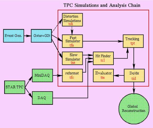
Figure 6.1: Schematic of the STAR TPC Software chain.

The procedure employed here is typical of that employed in many experiments. A flow diagram of the different software modules is depicted in Fig. 6.1. The chain is designed to cope with simulated and real data using the same code. We focus on the real data reconstruction. The details of the detector simulation (labelled “slow simulator” in Fig. 6.1) are discussed in Chapter 7.

One starts by examining the pixel information for every padrow independently in order to find the location where a charged particle has crossed the row, which we call a hit. A tracking algorithm then links together series of hits to find particle trajectories through the TPC volume. Information extracted from the ionization or from the topology of the tracks is then used for identification. We now discuss the reconstruction, emphasizing the two parts that are important for the charged hadron distributions discussed in this work: the determination of the momenta and the identification via $\frac{dE}{dx}$.

6.1.1 Cluster Finding

The hit reconstruction software converts raw pixel data into reconstructed space points. The raw pixel data is arranged into time ordered sequences for each pad in a row, where only pixels above a threshold are taken into account. At this stage, one must be careful to apply gain corrections and remove channels tagged by DAQ or previous offline runs as bad, noisy or dead. Any relative timing corrections between pads are also applied. The cluster finding algorithm then looks for contiguous pixels in a 2D space given by the time direction and the pad-row direction. After the 2D cluster finder stage, a pass is made to find single hits and multiple hits in a cluster. The single-hit finder assumes that the cluster is made by the crossing of a single track and estimates the centroid of the cluster. The multiple-hit finder tries to find the local maxima in a cluster and may deconvolute the cluster into individual hits. Deconvolution of close hits is of critical importance for two-track resolution and $\frac{dE}{dx}$ measurement. The fitted hits are then transformed into TPC space points, taking into account the drift velocity, trigger time offsets, sector geometry, and electronics shaper response. The space points then contain information on the position of the hit in the STAR global coordinate system and on the energy deposited by the track.

6.1.2 Track Finding

The detection of charged particle tracks is, of course, the raison d’être of a Time Projection Chamber. The track finding algorithm performs the critical task of converting the reconstructed space points into particle tracks, and of determining their 3-momentum. Efficient tracking and good momentum resolution are an essential part of the analysis presented here, and especially for analyses such as high-$p_{\perp}$spectra and resonance decay reconstruction.

The tracking algorithm starts with overlapping hits in the outer pad-rows as the track seeds. The first stage of the algorithm consists of a follow-your-nose approach which produces a collection of track segments, i.e. collections of space points associated with a track, either complete or partial. Once we have the segments, we perform an initial segment fitting, which incorporates multiple Coulomb scattering and energy loss in the gas. Outlier space points, i.e. hits that were assigned to the track in the segment finding stage but whose position lies far from the allowed track extrapolation error after the fitting stage, may be removed at this point. A further extrapolation of the tracks for purposes of segment joining is then executed, including also multiple Coulomb scattering and the effects of energy loss. The tracking parameters are updated for the joined segments and a clean-up of fragments is done in the final filtering step.

6.1.3 Particle Identification: $\frac{dE}{dx}$

The TPC allows us to separate pions using their ionization energy loss. The charge collected for each hit on a track is proportional to the energy loss of the particle. We parameterize the particle’s trajectory in order to obtain a path length in the gas which corresponds to each segment, i.e. the deposition that corresponds to a specific TPC hit. For a track crossing the entire TPC we thus obtain 45 $\frac{dE}{dx}$ samples, which are distributed according to the Landau probability distribution. One of the properties of this distribution is that its tail dies off very slowly, and the dispersion of values around the mean is very large (infinite in theory). A typical procedure in order to reduce fluctuations from the long Landau tails is to truncate the distribution. In the case of STAR, we used 70% truncation, i.e. the highest 30% ionization values were discarded. Using the remaining values, a truncated mean is computed, and this becomes the basis for any analysis using identified particles in the TPC. The measured truncated mean for negatively charged primary particles is illustrated in Fig. 6.2, shown as a function of the momentum.

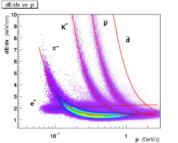
Figure 6.2: Particle identification via $\frac{dE}{dx}$ in the TPC. The plot shows the truncated mean $\frac{dE}{dx}$ value for negative tracks as a function of the reconstructed momentum. The expected ionization energy loss curves for $e^{-}$, $\pi^{-}$, $K^{-}$, anti-protons and anti-deuterons are also shown.

The curves are the Bethe-Bloch parameterization used in the analysis for the different particle hypotheses. We see that at the lowest momentum, the pions have a greater ionization energy loss than the electrons which are already in the saturation region of the curve. The pions cross over the electron band at $\sim 150\ \mbox{$\mathrm{MeV/}c$}$ reaching a minimum at about $300-400\ \mbox{$\mathrm{MeV/}c$}$. The pions in the relativistic rise merge with the Kaons, which are still in the $1/\beta^{2}$ region, at about 1 $\mathrm{GeV/}c$. However, due to the width of the bands, a single $\pi^{-}$ peak is only discernible up to $\sim 750$ $\mathrm{MeV}$.

$\frac{dE}{dx}$ Resolution

The $\frac{dE}{dx}$ resolution for this analysis was found to be $8.8\%$ for tracks with 45 fit points (31 $\frac{dE}{dx}$ samples after truncation). This is illustrated in Fig.6.3.

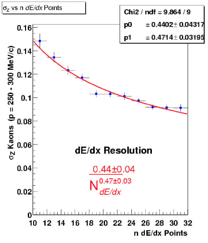
Figure 6.3: The $\frac{dE}{dx}$ resolution as a function of the number of $\frac{dE}{dx}$ samples.

A widely used empirical expression [140] describes the resolution at minimum ionization, for $N$ $\frac{dE}{dx}$ samples of length $h$ cm in argon gas with up to 20% CH₄ at a pressure of $P$ atmospheres:

$$\frac{\sigma_{dE/dx}}{\langle dE/dx\rangle_{\mathrm{trunc}}}=\frac{0.47}{N^{0.46}}(Ph)^{-0.32}=\frac{0.38}{N^{0.46}}$$ (6.1)

For the last equality, typical operation of the STAR TPC is at 1 atm and we assume the same radial pad length of $h=1.95$ cm (outer sector pads) for all ionization samples. Equation 6.1 then yields an estimate of the best achievable resolution of $\sim 7.8\%$ for tracks with 31 $\frac{dE}{dx}$ points. Improvements such as the removal of noisy pads, sector-by-sector calibration, and drift-distance dependence are expected to bring the resolution closer to this expected design value. These refinements are however not critical for the analysis presented here.

This is the first stage of the track finding and fitting pertaining to the TPC only. The information is then passed to the global reconstruction software, discussed next.

6.2 Global Event Reconstruction

There are two additional steps to arrive at the final tracks used in the analysis. The connection of the space point information among different detectors is the next step in tracking, i.e. a global track fit. This step becomes indispensable when including SVT or any additional information from a tracking detector. Finally, after the primary vertex is found, this acts as an additional measured point. If a track’s trajectory goes near the primary vertex, a subsequent primary track fit is then performed. For the analysis presented here, as we focus on production of primary charged hadrons, primary tracks are used.

The global event reconstruction offline software correlates all the tracking, timing and energy deposition information from each detector in STAR and produces the overall event characteristics of the triggered events into a Data Summary Tape format for use in all the physics analyses. We will discuss the major components here in roughly sequential form, although one sometimes performs several iterations among different modules. This is the case for example if one uses PID information in global track propagation, but would also want tracking information when calculating track segment lengths for the calculation of the specific ionization in a PID module. The flow of the global software chain is sketched in Fig. 6.4. The SVT is shown in the figure, although it was not yet installed for the 2000 run; we will therefore not discuss it here. The main objective of the global part of the chain however, is to combine the information from all STAR sub-detectors and was therefore exercised with simulated data to ensure readiness for real data.

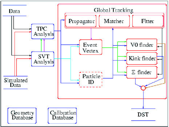
Figure 6.4: Schematic of the STAR Offline Software chain.

6.2.1 Global Tracking

The task of a global tracking module is two-fold. At its core, it is in charge of matching track and hit information from the different detector sub-systems. Once this is done, it must refit the newly matched tracks taking into account all available information. The role of the global tracking software was somewhat special for the 2000 run, since only 1 detector subsystem provided track information. In principle, one could then simply use the same TPC tracking parameters. However, since this would only be the case once, it was decided to actually perform a separate fitting routine at this level in order to work in a mode similar to that of having several sources of space point information.

The global tracking then really performed an independent track fit from the TPC. It used a 3D helix model and incorporated energy loss and multiple scattering in the TPC gas when doing the track propagation. The errors assigned to the space points were given by a parameterization, based on real data, of the hit residuals as a function of the track crossing angle with respect to the pad-row direction. This is also a case where one needs an iteration in order to have information flowing both ways: the tracking needs the errors in order to weigh each space point for a minimization routine to obtain the best track parameters, yet the hit errors depend on the crossing angle which is known once the track parameters are set.

6.2.2 Primary Vertex Finding

The offline reconstruction finds a primary vertex for each event by propagating the global tracks through the field towards some reference point which is close to the estimated vertex. One can choose a start point towards which to propagate the tracks either in the transverse plane or along the beam line. Since the interaction point is much better determined in the transverse plane (RMS $\sim 0.5$ mm) than along the beam axis (RMS $\sim 90$ cm). The method at the heart of the routine is a $\chi^{2}$ minimization of the perpendicular distances from the track vectors to a point. We can see the basis for this method in a simplified scenario where all the tracks are straight. In the transverse plane, the real vertex can only be a few millimeters away from the central axis. After propagating the helices to their point of closest approach to the reference point, we can then approximate them as straight lines around this point as in a Taylor series. This has the advantage of leading to an analytical solution. We consider then an arbitrary vector $V_{i}$, with a unit vector $\hat{e}_{V_{i}}$. The distance from a point $P=(x_{0},y_{0},z_{0})$ (in cartesian coordinates) to the vector $V_{i}$ is the norm of the vector obtained through the cross product of the unit vector $\hat{e}_{V_{i}}$ with any line connecting the point $P$ to any point $Q$ along the line of the vector $V_{i}$, $Q=(x_{i},y_{i},z_{i})$. The line segment $\overrightarrow{PQ}$ is $(x_{0}-x_{i})\hat{x}+(y_{0}-y_{i})\hat{y}+(z_{0}-z_{i})\hat{z}$, and the distance from $P$ to $V_{i}$ is

$$|d_{i}|=|\overrightarrow{PQ}\times V_{i}|\ .$$ (6.2)

A least squares minimization must employ a merit function ($\chi^{2}$) to assess the quality of the fit. We take the partial derivatives of the merit function with respect to the fit variables, and set them equal to zero in order to solve for the optimum values of the fit variables. For the vertex finder, the merit function is the summation of the squares of the perpendicular distances from the vectors $V_{i}$ to a point $(x_{0},y_{0},z_{0})$, with the appropriate weight given by the uncertainty in the propagation of the track,

$$\chi^{2}=\sum_{i=0}^{N}\frac{d_{i}^{2}}{w_{i}^{2}}\ .$$ (6.3)

By taking the partial derivatives with respect to $x_{0}$, $y_{0}$ and $z_{0}$ and equating them to zero, we are left with a system of three equations for three unknowns, the coordinates of the vertex $x_{v}$, $y_{v}$ and $z_{v}$.

The vertex finder then has two main components. One algorithm is used to extrapolate a helix and calculates the coordinates of the point of closest approach from a given point in the bend plane, defined relative to the $\vec{B}$ field which is along the beam axis. The transverse plane is defined perpendicular to the beam axis. The other task is to perform the least square fit to find the common vertex. Additional iterations can be performed such that the linearization is done as close to the actual vertex as possible, and rejecting outlier tracks in the fit. The details of the vertex finding algorithm are found in Ref. [141]

The vertex resolution for high multiplicity events is approximately 150 $\mu\mathrm{m}$, both perpendicular and parallel to the beam axis. The vertex finding efficiency is 100% for events with more than 50 primary tracks in the TPC acceptance, decreasing to 60% for those with fewer than 5 primary tracks. We discuss the vertex finding efficiency in more detail in Section 8.1.3 as it is an important part of the analysis of the multiplicity distribution.

6.2.3 Primary Track Fit

Once the vertex has been found, global tracks whose distance of closest approach to the vertex is less than 3 cm are chosen for a refit using the vertex as an additional space point, yielding as a result different parameters associated with primary tracks. For high multiplicity events, the error associated to the primary vertex is much smaller than the error associated to TPC space points, so even though we are only adding one additional point to the track it can significantly improve the momentum resolution for tracks that actually come from the vertex. This is the reason for choosing the primary track parameters for the analysis presented here. The track model in the STAR geometry and magnetic field can be to first order represented by a helix, which can be parameterized as

$$x = x_{0}+R\left(\cos(\Phi(s))-\cos(\Phi)\right)$$

$$y = y_{0}+R\left(\sin(\Phi(s))-\sin(\Phi)\right)$$ (6.4)

where $R$ is the radius of curvature, $\Phi=\psi+\pi/2$ and $\Phi(s)=\Phi-(s/R)*\cos(\lambda)$, and $s$ is the path length of the helix (see Fig. 6.5). The radius of curvature is related to the transverse momentum through

$$R = q/c$$ (6.5)

$$c = K\frac{qB}{\mbox{$p_{\perp}$}}$$ (6.6)

where $q$ is the charge of the particle, $c$ is the curvature, and $B$ is the magnetic field. With the following units: $B$ in KGauss, $p_{\perp}$ in $\mathrm{GeV/}c$, and $q$ in units of the proton charge; the value of $K$ to yield a curvature $c$ in cm is $K=0.000299$. The parameters that define the helix ($x_{0}$, $y_{0}$, $\psi$, $\lambda$, $q$, $c$) are obtained by two simultaneous 2D fits. We separate the fits in the bend plane and in the transverse plane, shown in Fig.6.5.

 

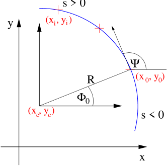
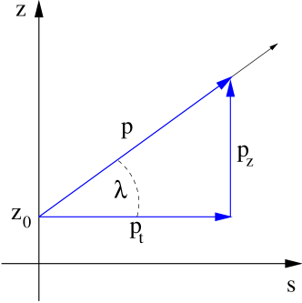
Figure 6.5: Projection of a helix onto the transverse plane (a) and onto the bend plane (b)

In the transverse plane, the space-points of a helix will project onto a circle, so the fit in the transverse plane ($x$ and $y$ coordinates in the STAR global coordinate system) is to a circle. In particular, the curvature of the track is obtained from such a fit, which relates to the transverse momentum as in Eq. 6.6. With the knowledge of the curvature, we can now focus on the fit in the bend plane. We can think of the helix as a string winding around a cylinder. If we cut the cylinder and unfold it into a plane, the helix segments will be mapped into straight lines in this plane. We then perform a straight line fit in the bend plane $z=(\tan\lambda)s+z_{0}$ where the coordinates for the fit are the path length ($s$) of the helix and the beam axis coordinates ($z$). The parameter $\lambda$ is called the dip angle in the helix parameterization, and it is identical to the polar angle $\theta$ in the definition of pseudorapidity, Eq. 4.17.

It is possible that secondary and decay tracks that are fit with the constraint of going through the primary vertex will have worse track parameters than those obtained from the global track fit. This is especially important for high-$p_{\perp}$ tracks, since biasing the tracks towards the primary vertex can artificially increase or decrease the curvature. For the majority of the tracks however, and in particular for true primary tracks, the resolution is improved by the primary track fit. Tracks for which the primary fit fails are flagged and not used in the analysis.

Momentum Resolution

The $p_{\perp}$ momentum resolution for $\pi^{-}$ for various multiplicities is shown in Fig. 6.6.

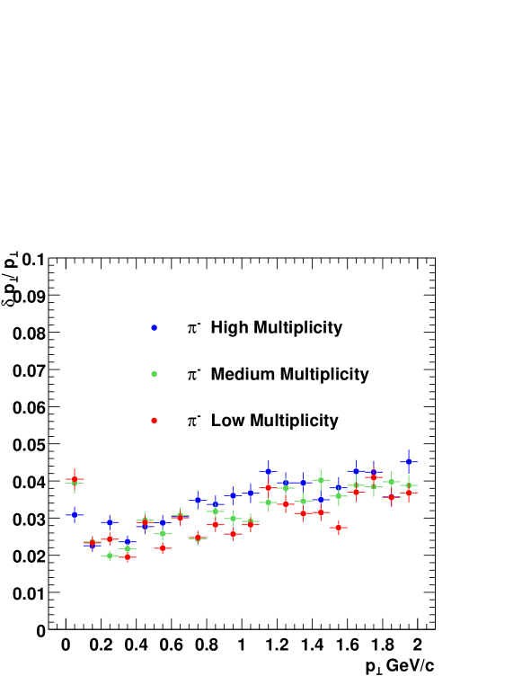
Figure 6.6: $\pi^{-}$ momentum resolution

This is obtained from embedding pions into real events using the TPC simulation discussed in the next section. The effects of the momentum resolution in the measurement of the $p_{\perp}$ spectra is discussed in Section 8.2.5.

6.2.4 $V_{0}$’s, $\Xi$’s, and Kinks

A specific part of the main STAR reconstruction code is dedicated to the topological identification of neutral and charged particle decays. Neutral particles such as the $K^{0}_{S}$ and $\Lambda$ can be reconstructed by identifying the secondary vertex, commonly called $V_{0}$ vertex, of their charged daughter decay modes, $\mbox{$K^{0}_{S}$}\rightarrow\pi^{+}\pi^{-}$ and $\Lambda\rightarrow p+\pi^{-}$. The more complicated “cascade” decay schema of the $\Xi$ and $\Omega$ baryons can also be reconstructed by a series of topological pattern recognitions using the $\Lambda$’s found in the first iteration through the decays: $\Xi^{-}\rightarrow\Lambda+\pi^{-}$ and $\Omega^{-}\rightarrow\Lambda+K^{-}$.

The charged kaon and pion one-prong decays found in the TPC volume are also reconstructed at this level ($K\rightarrow\mu+\nu$). The topology signature of this decay is that of a track which decays in flight while propagating in the gas of the TPC, with the daughter charged track following a slightly different direction, and is called a kink decay.

These steps are important for finding strange hadrons, i.e. $\lambda$ and $\Xi$ candidates using the $V_{0}$-finder algorithm and charged kaons using the kink-finder algorithm. In particular, the identification of charged kaons through the kink decay technique extends the available phase space to high momenta, where the $\frac{dE}{dx}$ measurement no longer has any resolving power. For recent results from the analysis of strange hadrons in STAR, see e.g. [90].

The secondary vertices are then reconstructed using the global tracks, propagating them towards the primary vertex and requiring that the $V_{0}$ vertex of the track pair should not be close to the primary vertex. In addition, when combining the pair momenta to obtain the momentum of the parent, one requires that the parent should point back to the primary vertex. This is the last important part of the global reconstruction. Additional pieces of the code mainly organize the reconstructed information into the STAR Data Summary Tape (DST) to be written to disk for further analysis. Although the main tuning of cuts to find secondary vertices is done at the analysis level, the initial stages of $V_{0}$ finding are done at the reconstruction level since part of the input are the space points, which are not saved to disk to minimize data volume. We turn our attention now to the TPC simulation.

Chapter 7 Detector Simulation

This analysis relies heavily on a realistic simulation of the response of the TPC. An estimation of the backgrounds and tracking efficiency is best done through such a simulation, and it is therefore necessary to include a significant amount of physics details. The primary function of the TPC Response Simulator (TRS) [142, 143] is to reproduce the electronic signals produced by tracks ionizing the gas of the TPC. The physical processes that are implemented are the drift of the ionized electrons in the gas, the amplification of the signal in the sense wires, the induction on the readout pads, and the response of the readout electronics which produce digitized data. While the software was designed to cope with varying levels of detail in each of the different simulation stages, we describe here the implementation that was used for the analysis stage in the past year.

7.1 Detector Response Overview

The algorithmic basis for the response simulations is that developed in detail by the ALEPH TPC group, described in Ref. [133], the standard reference for drift chambers. The TRS package contains parameterizations of the TPC response at various levels of detail.

As part of the requirements, TRS was designed to deal with two sources of ionization of the TPC gas: charged tracks and laser events. The charged tracks create clusters whose distribution of amplitudes (i.e. number of electrons in a cluster) is Landau-like, whereas the laser creates uniformly distributed ionization, resulting in Poisson distributed cluster amplitudes.

For the simulations used in the analysis, the magnetic field was taken to be uniform with a value of 0.25 T in the $z$ direction, and parallel to the electric field. During the analysis of the year 2000 data, several corrections needed to be applied to the raw data to take into account various distortion effects and modifications to the idealized geometry. These modifications were necessary for analyses such as the reconstruction of resonance decays and tracking of high $p_{\perp}$ particles. However, for the analysis of low momentum charged tracks up to 2 $\mathrm{GeV/}c$, these effects were negligible. The analysis was repeated every time new distortion and geometry corrections were added to the reconstruction chain and the results did not vary significantly. For example, a comparison of the measured raw multiplicity in the midrapidity region before and after distortion corrections using different event samples showed that they were consistent to better than 1 %. Therefore, it was sufficient to do the simulations in this idealized scenario.

There are four main processes that are essential for the simulation to reproduce the behaviour of a TPC.

• Ionization Transport – charge transport of the ionization and its deposition in the active region of the readout chambers.

• Charge Collection – electron/ionization collection on the sense wires of the multi-wire proportional chamber (MWPC).

• Analog Signal Generation – charge induction on the pad plane and generation of the time evolution of the analog signals on the pads.

• Digital Signal Generation – conversion of the analog signals into ADC counts.

We now discuss briefly each of the processes.

7.2 Ionization Decomposition and Transport

The input into the simulation of the TPC response is the charge ionization left by tracks in the sensitive volumes of the detector generated by GSTAR [144], the GEANT [145] implementation of the STAR detector. The ionization transport takes the charge deposited in these active areas of the detector and transports it through the field cage structure to the read-out plane. The GEANT simulation provides the amount of energy deposited ($dE$) over a given path-length ($ds$) by a particle with momentum $\vec{p}$. Given the average ionization potential of the gas, one can calculate the total number of electrons such that the transport can be done at the segment level ($dE$) or to break each segment into parts with the limiting case of transporting each ionization electron individually. This provides a mechanism which allows the possibility to distinguish between a detailed microscopic simulation and a macroscopic parameterization. In addition, one can also vary the length of the segment that is transported (and subsequently processed). Thus, the granularity of the simulation can be adjusted to provide different levels of detail.

The ionization is distributed on the pad plane according to distributions which characterize the effects of diffusion. The role of the charge transporter is to alter the $x$ and $y$ positions according to transverse diffusions, to alter the $z$ position to reflect the drift time with longitudinal diffusion folded in, and to alter the amount of charge that reaches the read-out plane.

7.3 Charge Collection and Amplification

Once the electrons arrive at the read-out plane, they must be collected by the individual anode/sense wires of the multi-wire proportional chamber (MWPC). It is here that the avalanche process multiplies the signal of several tens of electrons to several $10^{3}-10^{5}$ electrons, depending on the potential of the wires.

The basic principle of avalanche creation in a proportional wire is as follows. As an electron drifts toward the wire it travels in an increasing electric field. In the vicinity of the wire, the field $\vec{E}$ at radius $r$ is given by the linear charge density $\lambda$ on the wire

$$\vec{E}=\frac{\lambda}{2\pi\epsilon_{0}}\frac{\hat{r}}{r}.$$ (7.1)

The electron’s path is directed towards the wire. The trajectory also terminates in the wire in the presence of a magnetic field if the electric field is sufficiently strong. Once the electric field surrounding the electron is strong enough, the electron will have enough energy to ionize the gas and still pick up sufficient energy between collisions to ionize the gas further, starting an avalanche. The number of electrons continues to grow until all electrons reach the wire. The process develops over as many mean-free paths as there are generations of electrons, typically 50-100 $\mu\mathrm{m}$, and takes less than 1 ns for most gases. Since the signal is proportional to the number of electrons collected, the name “proportional wire” was adopted. For a review see [133] and [146] which also contains a list of texts.

The distribution of avalanches started by single electrons can be modelled as a stochastic process (see [133], p.144). A simple description is given by the Yule-Furry process, after the authors who first used it to describe biological population growth. The idea was applied to proportional avalanches by Snyder and Frisch (see [147] for references), and is briefly described in what follows.

We start from the idea that as the avalanche (or other stochastic process) develops, the variation of the number $n$ of ions (or electrons) is followed as a function of some parameter $t$. This parameter can be thought of as the time, but it is a bit more general in the sense that we need only require that its increase describes the progress of the process in the order given by the causal sequence of events. Therefore, $t$ need only be a monotonic function of time. We are interested in the probability $P(n,t)$ that at some ‘time’ $t$ there are $n$ electrons in the avalanche. The initial condition is that the avalanche starts with a single electron, i.e.

$$P(1,0)=1\ .$$ (7.2)

We suppose that the probability for the birth of one electron in any interval $\Delta t$ is proportional to the number of electrons $n$ with some proportionality constant $\lambda$. The solution to the corresponding differential equation giving the probability distribution at a given $t$ is

$$P(n,t)=e^{-\lambda t}(1-e^{-\lambda t})^{n-1}\ .$$ (7.3)

The mean $\bar{n}$ and the variance $\sigma^{2}$ are

$$\bar{n}=\sum_{n=1}^{\infty}nP(n,t)=e^{\lambda t}$$ (7.4)

$$\sigma^{2}=\sum_{n=1}^{\infty}n^{2}P(n,t)-\bar{n}^{2}=e^{\lambda t}(e^{\lambda t}-1)\ .$$ (7.5)

Rewriting 7.3 with 7.4 the distribution becomes

$$P(n)=\frac{1}{\bar{n}}\left(1-\frac{1}{\bar{n}}\right)^{n-1}\ ,$$ (7.6)

where the ‘time’ variable no longer appears. In the limit $\bar{n}\rightarrow\infty$, which is appropriate for avalanches, we obtain

$$P(n)=\frac{1}{\bar{n}}e^{-n/\bar{n}}\ ,$$ (7.7)

$$\sigma^{2}=\bar{n}^{2}\ .$$ (7.8)

We see that the Yule-Furry process has an exponential signal distribution. Subsequent theoretical refinements to this simple expression which were made in order to take into account effects like the asymmetric growth of the avalanche profile as well as saturation effects. One such refinement is the Byrne process, which introduces the idea that a fluctuation to larger $n$ in the first part of the avalanche reduces the rate of development in the second part (so an additional parameter has to be introduced, whose effect is to suppress the small amplification factors). The Byrne process includes the Yule-Furry process as a special case when the additional parameter approaches zero. The solution to the differential equations for this process is given by the Polya (or negative binomial) distribution function.

Exponential behaviour at low to moderate gas gains (i.e. $<10^{4}$) is observed experimentally. In parallel plate geometry however, slight deformation from exponential shape is observed at gas gains above $10^{5}$. This is probably due to self-saturation effects which become important in the presence of space charge. Since the STAR TPC is generally operated at low gas gains, the simple exponential is found to be acceptable for the simulations.

It is important to note that in any drift chamber operation, the effect of the fluctuations in gas gain is to simply degrade the attainable space-point resolution, and for this purpose it is not critical to use the exact functional form of the avalanche yields. The effect of degradation is the process that the simulation of the gas-gain fluctuation is attempting to reproduce, and the simple exponential should be sufficient in this regard.

Once the charge has been amplified, we can proceed to calculate the amount of charge induced on the cathode pad plane.

7.4 Analog Signal Generation

This simulation step has three main parts:

• Determination of the charge induced on single pads from the charge collected on the anode wires

• Sampling of the induced charge signals in time according to the electronics response (i.e. pre-amplifier and shaper)

• Distribution of the analog charge into time bins

7.4.1 Charge Induction

The charge induced on a grounded pad plane by a point charge $q$ located a distance $d$ above the plane can be calculated by the method of images. The charge density $\sigma$ on the plane is given by:

$$\sigma(x,y)=\frac{1}{2\pi}\frac{qd}{((x-x_{o})^{2}+(y-y_{o})^{2}+d^{2})^{3/2}}$$ (7.9)

where the charge is located at the position $(x_{o},y_{o})$. However, the typical geometry of a MWPC is a bit more elaborate. The proportional wires normally form a plane between two grounded cathode planes. In addition, the charge is not point-like, but in the form of a line of charge with density $\lambda$. We can simplify and locate it in the middle of the parallel plates. In order to calculate the charge density induced on the pad plane we thus have to include all higher-order multi-pole terms. The images are alternately negative and positive, situated at $z_{n}=\pm(2n+1)d$, $(k=1,2,\cdots)$ and $z_{o}=d$. The total charge density is obtained by integrating over $y$ and doing the sum

$$\sigma(x)=-\frac{\lambda}{\pi}\sum_{n=0}^{\infty}(-1)^{n}\frac{(2n+1)d}{(x-x_{o})^{2}+(2n+1)^{2}d^{2}}=-\frac{\lambda}{4d\cosh\left(\frac{\pi(x-x_{o})}{2d}\right)}$$ (7.10)

which is called the Endo function. The derivation was done without taking into account the limited extent of the pads in the y direction, i.e. for the limiting case of zero width to length ratio $w/l$.

The effect of finite geometry of segmented cathodes can be taken into account with the addition of another parameter. We can rewrite Eq.7.10 as

$$\sigma(x)=C_{1}\frac{1-\tanh^{2}\left(\frac{\pi(x-x_{o})}{4d}\right)}{1+\tanh^{2}\left(\frac{\pi(x-x_{o})}{4d}\right)}$$ (7.11)

where $C_{1}$ is a normalization constant. Eq. 7.11 can be used to generalize the Endo function to take into account finite geometry effects due to segmented cathode pads, i.e. $w/l>0$. By introducing the constant $C_{2}$

$$F(x)=C_{1}\frac{1-\tanh^{2}\left(\frac{\pi(x-x_{o})}{4d}\right)}{1+C_{2}\tanh^{2}\left(\frac{\pi(x-x_{o})}{4d}\right)}$$ (7.12)

we arrive at the generalized solution to the distribution of charge induced on a grounded pad plane, and is usually dubbed the Gatti function.

A comparison of the Gatti and Endo functions, along with a Gaussian (for comparison purposes) is given in

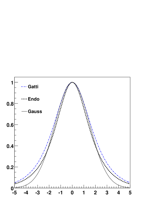
Figure 7.1: Comparison of Gatti, Endo and Gaussian functions as profiles of the pad-response function.

Figure 7.1. For reference, the functions were normalized to 1 at $x=0$ for the plot and the parameters were $\sigma=1.5$ for the Gaussian, $d=2$ for the Endo function and $d=2$, $C_{2}=0.5$ for the Gatti function.

For the case of the TPC, the quantity of interest is the total amount of charge ($Q$) induced per pad, so we have to integrate a given pad-response function, which gives the charge density, over the area of a pad:

$$Q=\frac{1}{2\pi}\int_{y_{l}}^{y_{u}}\int_{x_{l}}^{x_{u}}\sigma(x,y)dxdy$$ (7.13)

The advantage of using such functions is that they allow the production of longer tails which have non-Gaussian characteristics. The tails are an important feature to understand, as they determine the efficiency of the ionization collection which is of relevance in the study of $\frac{dE}{dx}$ resolution. As an additional case, the pad response function was measured for the STAR TPC pads in the directions transverse to and parallel to the anode wires. This allows us to calculate the pad response as a convolution of the transverse diffusion function with a parameterization of the measured pad response function.

7.4.2 Sampling of Signal in Time and Shaper Response

Once the amount and centroid of the charge distribution on each pad is determined, this charge can be sampled in time, thereby emulating the response of the analog electronics. The signals are generated by superimposing each analog signal from each of the avalanches that induce a signal on the pad plane. This permits one to vary the shaping time of the electronics independently of the width of the pad response function. In reality, the time evolution of the signal that develops on the wires is almost entirely due to the motion of positive ions away from the wire. This produces a signal with a long tail. For the STAR geometry, the duration of this signal is on the order of $\sim 62\ \mu$s. In order to make the detector faster, the signal is differentiated after a characteristic time – the shaping time of the pre-amplifier. The trade-off is that only a fraction of the total charge is seen by the downstream electronics, i.e. the ADC. The fraction $F$ of the charge is given by

$$F=\frac{\ln\left(1+\frac{t_{m}}{t_{o}}\right)}{\ln\left(1+\frac{t_{s}}{t_{o}}\right)}$$ (7.14)

where $t_{m}$ is the length of time the long, undifferentiated signal would persist ($\sim 62\ \mu$s), $t_{o}$ is the characteristic time of the development of the signal ($\sim 1\ \mu$s) and $t_{s}$ is the shaping time of the pre-amplifier ($\sim 180$ ns).

For STAR this means that the signal shape is dominated by the shaping properties of the electronics. Therefore, the long time response of the chamber is parameterized in the electronics processing section of the simulator, instead of modelling the motion of the positive ions. The shaper response function for the case of one stage differentiation and two stage integration used in STAR is

$$g(t,\tau)=\Phi(t)\left(\frac{t}{\tau}\right)^{2}e^{-t/\tau}$$ (7.15)

where $\Phi(t)$ is the step function, and the time constant $\tau$ is 55 ns for the STAR electronics. This function is then convoluted with a Gaussian to parameterize the effect of a longitudinally diffused cluster to yield the final response of the shaper.

Once we obtain the functional form of the signals induced on a pad over the read-out period of the TPC electronics, we can distribute the analog signal into discrete time bins. This sampling simulates the behaviour of the Switched Capacitor Array (SCA) in the front end electronics. Essentially, this entails integrating the amount of charge in a time interval $\Delta t$, which is determined by the SCA sampling frequency. Simulated chamber noise and electronic noise are also added at this point.

7.4.3 Digital Signal Generation

Once the analog charge is distributed into time bins on the pads, we can digitize the signal. This step is done via a simple conversion from voltage to ADC counts. This is the final stage in the TPC simulation, and the pixel values are then used as input to the reconstruction chain in exactly the same way as the raw data.

7.5 Embedding

One of the main purposes of the detector simulation response is to obtain estimates of tracking corrections to the raw particle yields. It is of great importance to have a reliable detector simulation as detailed in the previous section. To make the environment as realistic as possible, we use a procedure commonly known as embedding. The idea is to take a real event and embed into the raw data file the signal from a few simulated tracks at the level of ADC counts. The simulated signal is obtained via a GEANT Monte Carlo simulation of the energy deposited by the tracks in the detector volume followed by a simulation of the detector response as detailed in the previous section. The final simulated ADC signal is then convoluted with the raw data from the real event and then fed into the STAR reconstruction software chain. Since we have the information from the GEANT simulation, we can associate the reconstructed tracks to the corresponding Monte Carlo track. The association is done at the hit level, since from the reconstruction side the hits are the “seed” from which the track parameters are built.

The embedding procedure combines the advantages of having a very realistic event environment along with having a controlled track population. From the comparison of reconstruction output to simulated input we can obtain information about many interesting performance diagnostics of the detector.

Figure 7.2 shows the position resolution for hits in the TPC in the drift direction. The RMS width is found to be 180 $\mu\mathrm{m}$, a similar analysis in the padrow direction yields an RMS width on the order of 120 $\mu\mathrm{m}$.

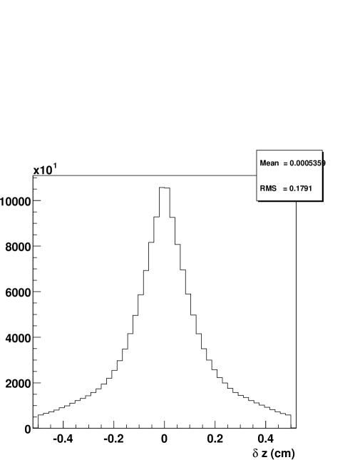
Figure 7.2: TPC hit position resolution in the drift direction.

Once we have a match between the TPC hits, we can use this information to make a matching between tracks. For every reconstructed track, we scan through its reconstructed space points and find their corresponding Monte Carlo hits. These simulated hits have the necessary information of the track that generated them, and so form the basis for the track match. It is this track match information that we use for the determination of the reconstruction efficiency. We discuss the corrections to the raw spectra obtained through the embedding procedure and through background simulations in the next chapter.

Chapter 8 Analysis of Charged Hadron Spectra

8.1 Event-wise Studies

In this section we delineate the relevant parts of the analysis that was performed to obtain the multiplicity distribution. This is also the baseline for any other analysis.

8.1.1 Trigger and event selection

We use the ZDC and the CTB for triggering. All the runs that we used for this analysis were recorded with a minimum bias trigger, with no pre-scale. The minimum bias trigger consisted of a coincidence requirement between the East and West ZDC’s. This trigger proved to be better than 99% efficient. At the beginning of the run, however, this had yet to be established. The main concern was that there might be an inefficiency in this trigger for the most central collisions, where very few spectator nucleons remain to produce a coincidence in the calorimeters. Therefore, a high CTB signal, indicative of a high multiplicity in the mid-rapidity region, was used as an additional trigger condition. The ZDC trigger thresholds were set such that a single nucleon hitting the calorimeter would generate an acceptable signal. The CTB threshold was set to accept the highest $\sim 30\%$ multiplicities.

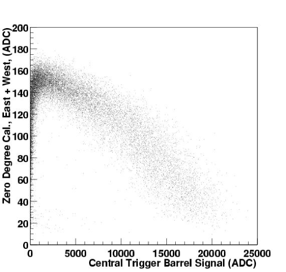
Figure 8.1: The ZDC (sum of East and West calorimeters) signal is plotted vs. the corresponding CTB signal. The most central events have the highest CTB signal (high multiplicity) and a low ZDC signal (very few spectator neutrons).

A plot of the ZDC vs. CTB trigger signals for a subset of the events used in this analysis is shown in Fig. 8.1. The peripheral collisions are in the lower left corner, where both the CTB signal and the sum of the East and West ZDC signals are small. This is indicative of low multiplicity at mid-rapidity and a scarce number of dissociation neutrons. In the collider geometry, neither the excited nucleus nor the dissociation protons reach the calorimeters because their trajectories are bent by the beam optics. As the overlap of the colliding nuclei (i.e. the centrality) increases, more neutrons reach the calorimeters and the ZDC signal increases. Likewise, the multiplicity at mid-rapidity increases. After a certain point, the collision is sufficiently central that few neutrons reach the ZDC while the multiplicity continues to increase. The “boomerang” shape observed in Fig. 8.1 is therefore the result of the correlation between impact parameter $b$ and multiplicity on the CTB side, and of a dual behaviour on the ZDC side: correlation between $b$ and number of neutrons at high impact parameter, and anti-correlation for central collisions.

An important input into this analysis is the hadronic cross section in $\mathrm{Au}+\mathrm{Au}$, $\sigma_{\mathrm{AuAu}}$. This value is necessary to normalize the multiplicity distribution. The calculated value is $\sigma_{\mathrm{AuAu}}$ = 7.2 barn from Eq. 4.8, but it is desirable to have a measurement confirming this expectation. The trigger requirement of a ZDC coincidence is not only sensitive to the hadronic cross section, but also to the mutual Coulomb dissociation of the two Au nuclei. In this process, there will be a pair of correlated forward- and backward-going neutrons, but no measurable tracks in the mid-rapidity region. The ZDC’s therefore are sensitive to the sum of the hadronic + mutual Coulomb dissociation cross sections, which we denote by $\sigma_{xn,xn}$, i.e. the cross section in which at least one neutron is detected in each ZDC detector. Since the same ZDC’s are used in all interaction zones at RHIC, this combined cross section can be measured by all 4 RHIC experiments independently. The STAR preliminary result, measured by the van der Meer scan technique [148] is $\sigma_{xn,xn}=8.9\pm 0.3_{\mathrm{stat}}\pm 0.7_{\mathrm{sys}}$ barn. This value has also been measured in an independent analysis by the RHIC accelerator crew [149]. The value reported in a calculation [150] is $\sigma_{xn,xn}=10.9\pm 0.6$ barn, and seems to be outside of the allowed range of the systematic uncertainty in the measurements. Attempts to resolve this discrepancy are underway. In order to arrive at a measured hadronic cross section, $\sigma_{\mathrm{AuAu}}$, it is also necessary to disentangle the contributions from the hadronic and the Coulomb processes. Since a $p\bar{p}$ inelastic collision at $\sqrt{s}$ = 130 $\mathrm{GeV}$ produces on average $\sim 2.4$ (see Eq. 4.11) charged particles per unit pseudorapidity at mid-rapidity and we expect to identify the vertex for hadronic events, to first order this fraction can be measured as

$$\frac{\mbox{$\sigma_{\mathrm{AuAu}}$}}{\sigma_{xn,xn}}=\frac{\mathrm{Events\ with\ Vertex}}{\mathrm{Total\ Triggered\ Events}}$$ (8.1)

This simple ratio must be corrected for the vertex-finding efficiency and acceptance that reduce the counts in the numerator and for backgrounds such as beam+gas that generate a trigger and are therefore counted in the denominator. The vertex finding efficiency is important in this analysis and for the determination of the shape of the $h^{-}$ multiplicity distribution at low multiplicity.

8.1.2 Vertex Acceptance

The vertex reconstruction for the summer 2000 run was undertaken essentially up to the limits of the TPC acceptance, i.e. $|\mbox{$z_{\mathrm{vertex}}$}|<2$ m where $z_{\mathrm{vertex}}$ denotes the position of the primary vertex along the $z$ direction parallel to the beam. Although it is possible to try to obtain a vertex as long as there are tracks in the TPC, this was not pursued for the following reasons. If an event occurred outside of this region, the TPC sees only the forward- or the backward-going particles. This also has the disadvantage of reducing the accuracy of the vertex determination, since the $z$ position of tracks going perpendicular to the beam axis contribute significantly to the determination of the vertex. In addition, the CTB in this case is not triggered on multiplicity at mid-rapidity, but rather on multiplicity forward or backward of mid-rapidity with all tracks having a large dip angle. To avoid these systematic effects, the vertex finder was set to abort when it determined that the vertex lay outside the TPC limits.

Due to the large size of the beam diamond, the standard deviation of the vertex Z position was $\sim$ 100 cm. This results in valid collision events, even at high multiplicity, without a vertex determination. In addition, in order to keep a flat acceptance for tracks with $|\eta|<0.5$, we restricted the multiplicity analysis to events with a vertex between $\pm 95$ cm, about a $\pm 1\sigma$ cut. To correct for the vertex acceptance, we assume that the distribution is Gaussian and from the fit parameters estimate the fraction of events that lie outside our acceptance cut. As an example, the $z_{\mathrm{vertex}}$ distribution for 10K triggered events from one of the runs taken in September 2000 is shown in Fig. 8.2.

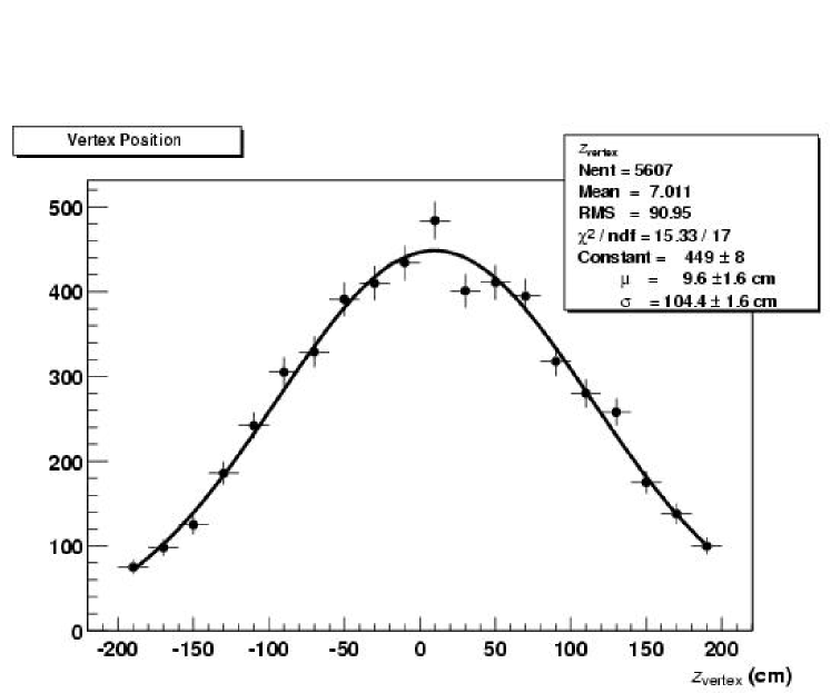
Figure 8.2: Distribution of reconstructed vertex $z$ positions, $z_{\mathrm{vertex}}$, for 10,000 triggered events. The limits of the TPC are at $\pm$2 m from the center. The acceptance for events used in the multiplicity analysis was placed at $\pm 95$ cm.

For the distribution in Fig. 8.2, the acceptance correction factor is 1.57. Analyzing more runs for a total of 166K triggered events, we find an acceptance correction factor of 1.68, (a $\pm 1\sigma$ cut for a Gaussian distribution would yield a correction of 1.46, so our cut is tighter). With the vertex efficiency and acceptance correction, we can then determine the numerator in Eq. 8.1. For the denominator, we must estimate the backgrounds to our minimum-bias trigger.

8.1.3 Vertex Efficiency

We know that our offline vertex reconstruction is not 100% efficient, therefore we need to correct for this effect when measuring the multiplicity distribution. The vertex reconstruction is based on tracing the path of reconstructed tracks back to a common space point. Since tracking is done first, before finding the vertex there is no a priori knowledge of which tracks are primary and which ones are not. The vertex-finding therefore depends on all global tracks (Sec.  6.2.1) found in the event. We will then characterize the efficiency as a function of the number of global tracks ($N_{\mathrm{global}}$) in the event. The vertex-finding efficiency ($\epsilon_{\mathrm{vtx}}$) affects mainly the low multiplicity events. The reason is that these events provide the vertex-finding algorithm with very little information to work with, i.e. very few global tracks. We find that for events with more than $\sim 100$ global tracks, the efficiency is $\sim 100\%$. To confirm the findings based on software, a visual analysis of $\sim 100$ events was performed, with a resulting lower bound on the efficiency for events with $N_{\mathrm{global}}$ = 100 of $\epsilon_{\mathrm{vtx}}$  > 98%.

The more important part is the efficiency at low $N_{\mathrm{global}}$. To get a handle on this number, we used hijing events generated with large impact parameter $b$ = 12 - 20 fm. At these impact parameters, hijing should be a reasonable model, since basically only geometry and the $pp$ cross section play a role and nuclear specific effects are not expected to influence the results. These events were then processed through the STAR reconstruction chain and a record was kept of the number of events generated and whether the vertex was or was not found for each event. In this way, we obtain a plot of the vertex efficiency correction factor (1/$\epsilon_{\mathrm{vtx}}$). The correction depends on $N_{\mathrm{global}}$ and is illustrated in Fig. 8.3.

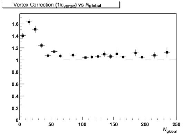
Figure 8.3: Vertex finding efficiency correction factor as a function of the number of global tracks, $N_{\mathrm{global}}$.

To take this correction into account in the $h^{-}$ multiplicity distribution, the correction in Fig. 8.3 was used as a weight for each event depending on the number of global tracks. Since the $h^{-}$ multiplicity distribution refers to negative primary tracks instead of global tracks, this correction affects primarily the region $N_{h^{-}}$ < 5 and is negligible beyond $N_{h^{-}}$ = 10. These are the first two bins of the final distribution. However, most of the cross section is found in these bins, and the shape of the distribution is sensitive to these values at low multiplicity. To figure out what is the fraction of the hadronic cross section that we actually see, we proceed as follows. We choose events within a $\pm 95$ cm range along the $z$ axis of the beam direction. We can then count the the raw number of events with vertex in our multiplicity distribution. We compare this to the number of vertex events corrected for efficiency, i.e. to the number of events in the multiplicity distribution appropriately weighted with the correction from Figure 8.3. From these two numbers, we see that the fraction of the hadronic cross section available to the offline analysis is $94.9\pm 0.5\ \pm 4\ \%$ of $\sigma_{\mathrm{AuAu}}$, where the systematic uncertainty comes from the uncertainty in the estimation of the vertex efficiency at the lowest multiplicities based on the simulations.

8.1.4 Trigger backgrounds

We now focus on estimating the contribution to the events in the denominator in Eq. 8.1 that are not part of the total $\sigma_{xn,xn}$ cross section, e.g. beam-gas events. However, knowing which events are background so that we can take them out of our total trigger sample, is not trivial.

To investigate this issue, we focus on events for which the vertex was not found. To study systematic effects and variations, from the September data, we used specific minimum bias runs with good statistics, and stable detector operation. The run with the most statistics in this period has $\sim$ 77K events (the events in Fig. 8.2 is from this sample). This was used along with a few other runs to compare backgrounds and other systematic effects.

For these background studies, we compared 4 runs with different luminosity conditions spread over several weeks. Two of these (August 2000 data) had intensities in RHIC which were about a factor of 3 lower than in the other two (September 2000) runs. We are interested in the different intensities because the hadronic interaction rate grows as the product of the intensity in each beam, while the beam+gas background grows only as the sum. This type of background should then have a different contribution in runs with differing beam intensities.

To illustrate the difference between the events with and without vertex, a plot of the trigger information from 10K events from one of the runs is shown in Fig. 8.4 Events with a reconstructed vertex are shown in the left panel; the right panel illustrates the trigger signals for events without a reconstructed vertex.

 

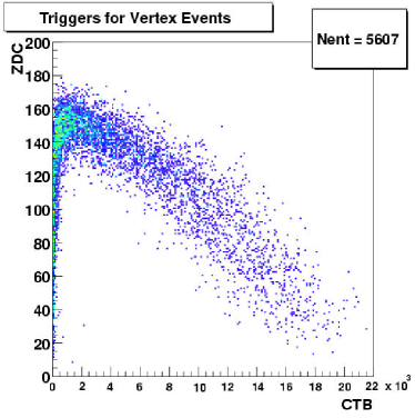
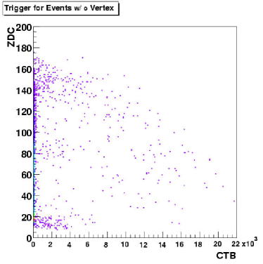
Figure 8.4: The trigger signal for events with a valid reconstructed vertex (a) shows the expected shape. There are additional event classes that show up when plotting the trigger signal for events without a reconstructed vertex (b).

For events in Fig.8.4(a), we see again the very clean “boomerang” band. These represent valid hadronic events for the determination of $\sigma_{\mathrm{AuAu}}$. For the events without a reconstructed vertex, there are several regions to understand. The events which lie in the “boomerang” are most likely good events that did not have a vertex because the collision occurred outside the bounds of the TPC, where the acceptance of the offline vertex finder terminates. This does not present a problem. However, in the 2001 run a cross check will be done using timing in the ZDC’s. There are two other regions that are most probably background and have been the subject of further scrutiny:

• ZDC < 30 (low ZDC region)

• ZDC $\sim$ 80 (mid ZDC region)

Both of these regions have events whose trigger signals extend along the CTB axis. If the multiplicity is increasing for these events, we should see also an increase in the number of global tracks. The same thing is found if we plot the ZDC signal vs. $N_{\mathrm{global}}$for the events with and without vertex, shown in Fig. 8.5.

 

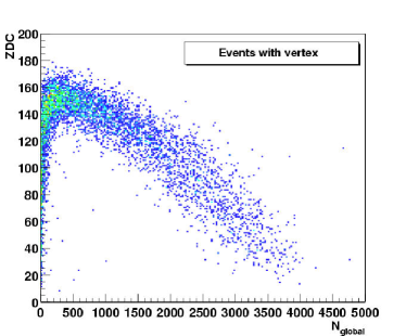
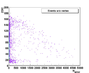
Figure 8.5: The ZDC signal vs. the number of global tracks for events with a valid reconstructed vertex (a) and without one (b). The same structure as in Fig. 8.4 is seen, indicating that there is definitely an increased number of charged tracks in the detector for the events in the two regions outside the “boomerang”.

We see that there are events that have $\sim$ 1000 global tracks, do not have a reconstructed vertex and lie in a different region than the normal hadronic events.

We studied the characteristics of these two bands to try to understand their origin. We investigated other differences between these bands and the rest of the “good” triggers to shed light on their nature. We expect that in the region $N_{\mathrm{global}}$$\leq 1$ most of the events are of electromagnetic origin. In any case, there can be no vertex reconstructed for events with less than 2 tracks. By selecting non vertex events with $N_{\mathrm{global}}$>1 we focus on the possible backgrounds the we’re aiming to understand.

We find that the band at low ZDC has both East and West ZDC triggers just above threshold, and the band in the mid ZDC region has one of the calorimeters just above threshold and the other one high. For the ZDC $\sim 80$ region, this is just the opposite behaviour than is seen in the events with a found vertex, where the ZDC signal is relatively symmetric between East and West ZDC’s. It is possible that a beam+gas event could generate such an asymmetric ZDC signal with some charged tracks seen in the TPC. Asymmetries in tracking were also found, but this can also indicate simply an interaction outside the TPC volume. Several hypotheses were proposed, but there was insufficient information to unambiguously discern the nature of the background. In particular, we would like to know its contribution to the region where the valid events lay. Without this knowledge, we can remove only the background contribution outside the “boomerang” region. We can therefore only produce a lower limit on the fraction in Eq. 8.1. The numerator depends on the efficiency and acceptance corrections already discussed. For the purpose of the calculation of the fraction, we used events within $\pm 2$ m to reduce the acceptance correction ($6\%$). For the denominator, we start with the total triggers. The background is obtained via the number of events without vertex that have 1 or more global tracks. Since some of these events are valid events that were not found because of efficiency or acceptance, we need to subtract the number of events we added to our numerator due to these two corrections from the background estimate. This is a lower bound since we don’t take into account the background for events without global tracks. From 10K events from the low luminosity runs and from 15K events from the high luminosity runs we obtain

$$\mathrm{Low}\ \mathcal{L} : \frac{\mbox{$\sigma_{\mathrm{AuAu}}$}}{\sigma_{xn,xn}}\geq 70.0\pm 0.7\ \%$$

$$\mathrm{High}\ \mathcal{L} : \frac{\mbox{$\sigma_{\mathrm{AuAu}}$}}{\sigma_{xn,xn}}\geq 73.5\pm 0.6\ \%\ .$$ (8.2)

The errors are statistical, which is enough to compare the two numbers since they were obtained in the same way. We can see that there is a difference beyond statistical. However, this was expected as the low-luminosity runs systematically have a greater background contribution that our procedure does not account for. For the high-luminosity sample, this background is reduced and the lower limit on the fraction is higher. Using the fraction from the high-luminosity events and the current measured value for $\sigma_{xn,xn}=8.9\pm 0.5$ barn, we obtain a lower limit on the hadronic cross section $\sigma_{\mathrm{AuAu}}\gtrsim 6.5$ barn, consistent with the calculated value of 7.2 barn. There should be an error of $\pm 0.4$ barn in this estimate which comes basically from the cross section measurement (the statistical error on the fraction is much smaller). This error in turn is dominated by the uncertainty in the measurement of the beam currents in the RHIC ring, which is on the order of 3%. The systematic uncertainty on the fraction is the only missing piece, but as discussed, at this point we can only give a lower bound.

It is clear that with only the ZDC and CTB information at the lowest multiplicities, it becomes increasingly difficult to separate the background events such as beam+gas collisions. It would therefore be of great advantage to obtain an estimate of the interaction point without having to rely on tracking, but rather on trigger signals, e.g. on timing between the arrival of the East and West ZDC signal. In addition, improved phase space coverage for the trigger would drastically reduce uncertainties in the background estimates and help to provide a more complete topology of the valid low multiplicity hadronic events. For the 2001 run ZDC timing will be implemented; and starting with the 2001 $pp$ run, additional detectors in the form of scintillator slats covering from the pseudorapidity region $2<|\eta|<4$ will be part of the STAR trigger as well. For the analysis of the multiplicity distribution presented in Sec. 9.1 we will use the calculated value of the $\mathrm{Au}+\mathrm{Au}$ hadronic cross section of $\mbox{$\sigma_{\mathrm{AuAu}}$}=7.2$ barn for the normalization.

To obtain the multiplicity distribution, one has to obtain the corrected number of negative hadrons for every event. The analysis done here relies on tracking. We first obtain a raw $dN/d\mbox{$p_{\perp}$}d\eta$ distribution as a function of $\eta$ and $p_{\perp}$ for every event. Then several corrections are applied to this raw distribution as discussed in the next section. Finally, the corrected $dN/d\mbox{$p_{\perp}$}d\eta$ distribution is integrated in the range $|\eta|<0.5$, $0.1<\mbox{$p_{\perp}$}<2\ \mbox{$\mathrm{GeV/}c$}$ to obtain a corrected multiplicity. One can therefore also obtain $p_{\perp}$ and $\eta$ distributions with this procedure. Since the algorithm relies on tracking corrections, we now turn our attention to this subject.

8.2 Tracking Studies

Particle production was studied through the yield of primary negative hadrons, which are mostly $\pi^{-}$ with an admixture of $K^{-}$ and $\bar{p}$. The $h^{-}$ distribution includes the products of strong and electromagnetic decays. Negatively charged hadrons were the main focus of the work in order to exclude effects due to participant nucleons which would show up in the positively charged hadron sample. Charged particle tracks reconstructed in the TPC were accepted for this analysis if they fulfilled requirements on number of points on the track and on pointing accuracy to the event vertex.

The main goal of this analysis is to determine the corrected yield of primary particles coming from the collision. What we have in the final state are measured tracks, both primary and secondary, in our detectors. There are several losses and backgrounds that need to be corrected: acceptance, decay losses, track reconstruction efficiency, contamination due to interactions in material, misidentified non-hadrons, and the products of weak decays. The appropriate corrections were obtained mainly by use of the embedding technique. Backgrounds were determined by either fully simulated events or by direct measurement when possible. All corrections were calculated as a function of the uncorrected event multiplicity. The corrections used in the determination of the final spectra are obtained in the following order:

1. Geometrical acceptance and decay losses

2. Reconstruction efficiency

3. Track merging

4. Momentum resolution

5. Track splitting

6. Electron background

7. Weak decay and secondary interaction background

8. Ghost tracks

We now discuss the most important corrections in more detail.

8.2.1 Acceptance

The acceptance correction takes care of two different things. What we really focus on here is whether or not a charged particle makes a measurable signal in the detector such that it is possible to reconstruct it afterwards. If the charged particle does not deposit energy in any sensitive volume of the detector, it will be lost. This is the more common definition of the geometrical acceptance. In addition, a charged particle may also leave no signal if it decays in flight before it reaches the detector. In the STAR Monte Carlo simulation implemented for this work, these two losses were taken into account simultaneously by adopting the following definition of acceptance: a track is accepted if it leaves at least 10 Monte Carlo hits in the TPC. The reconstruction code then at least has the possibility to find the track. This correction can be calculated in a full Monte Carlo simulation and also using embedding, and should be completely independent of the event multiplicity. There should be a dependence on particle type, as the decay characteristics are included in our definition. This is illustrated in Fig. 8.6.

 

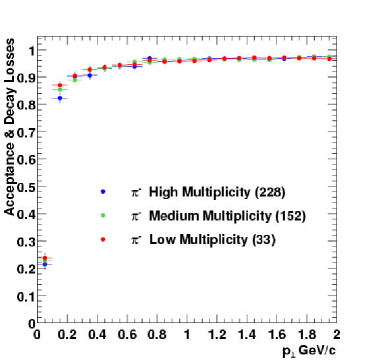
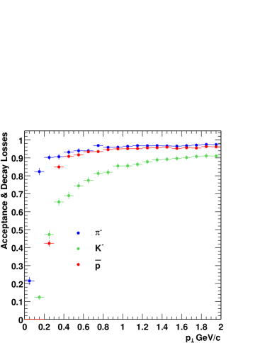
Figure 8.6: The acceptance correction for the $h^{-}$ analysis. Left panel: $\pi^{-}$ acceptance for 3 multiplicity selections. Right panel: Acceptance for $\pi^{-}$  $K^{-}$ and $\bar{p}.$

The left panel is the acceptance for negative pions in three multiplicity bins. The numbers correspond to the mean raw negatively charged multiplicity ($\langle\mbox{$h^{-}$}\rangle_{\textrm{raw}}$) in each of the 3 bins: $\langle\mbox{$h^{-}$}\rangle_{\textrm{raw}}=223$ for the high multiplicity, $\langle\mbox{$h^{-}$}\rangle_{\textrm{raw}}=152$ for medium, and $\langle\mbox{$h^{-}$}\rangle_{\textrm{raw}}=33$ for the low multiplicity bin. The plot shows that the correction is essentially independent of the multiplicity, except perhaps at the lowest $p_{\perp}$. The right panel is the acceptance for the three particle species which make up the $h^{-}$ distribution. We see that the $K^{-}$ acceptance is lower than that for the pions, which is expected since $c\tau=3.7$ m for kaons, and it is 7.8 m for $\pi^{-}$.

The acceptance is on average 90% for tracks within the fiducial volume having $\mbox{$p_{\perp}$}>200$ $\mathrm{MeV/}c$. We see that the acceptance rapidly drops at low $p_{\perp}$. For the $h^{-}$ analysis, we accept tracks which have $0.1<\mbox{$p_{\perp}$}\,<2$ $\mathrm{GeV/}c$ and $|\eta|<1.0$. This accounts for the majority of the produced particles at mid-rapidity, as we find the yield beyond $p_{\perp}$ = 2 $\mathrm{GeV/}c$ to be only 1% of the total yield. A motivation to go as low in $p_{\perp}$ as possible was driven by the fact that for 2001 the magnetic field would be set to the design operating value of 0.5 T for the bulk of the data taking, instead of the 0.25 T used in 2000. This raises the low-$p_{\perp}$ acceptance of the TPC, so essentially the 2000 data would give us access to the lowest $p_{\perp}$. Nevertheless, to study systematic effects the multiplicity analysis was carried out three times with various low-$p_{\perp}$ cutoffs: $p_{\perp}$>0 (no cutoff, large systematics expected), $p_{\perp}$>0.1 $\mathrm{GeV/}c$ and $p_{\perp}$>0.2 $\mathrm{GeV/}c$ yielding consistent results.

8.2.2 Tracking Efficiency

Once a track has made it into the detector, we focus on the question of how likely it is to be found by the offline software chain. The reconstruction efficiency was determined by embedding simulated tracks into real events at the raw data level, reconstructing the full events, and comparing the simulated input to the reconstructed output. This technique requires a precise simulation of isolated single tracks, achieved by a detailed simulation of the STAR apparatus based on GEANT and a microscopic simulation of the TPC response discussed in Chapter 7. The multiplicity of the embedded tracks was limited to 5% of the multiplicity of the real event in the same phase space as the simulated data, thereby perturbing the real event at a level below the statistical fluctuations within the event sample. Fig. 8.7 shows the reconstruction efficiency obtained from embedding as a function of $p_{\perp}$ for a slice at mid-rapidity.

 

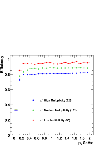
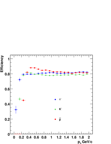
Figure 8.7: The reconstruction efficiency for the $h^{-}$ analysis. Left panel: $\pi^{-}$ efficiency for 3 multiplicity selections. Right panel: Efficiency for $\pi^{-}$, $K^{-}$ and $\bar{p}$ at high multiplicity.

The tracking efficiency varies depending on $p_{\perp}$ and the multiplicity of the event. For the lowest multiplicity events, the $\pi^{-}$ efficiency is $\gtrsim 95\%$ in the region $p_{\perp}$ > 400 $\mathrm{MeV/}c$. Going to the high multiplicity events degrades the efficiency to $\sim 80\%$. However, since the difference between the multiplicities in the high and low bins is about a factor of 7, a reduction of only $\sim 15\%$ in the efficiency is a significant achievement for the offline reconstruction. In general, for all multiplicities and all 3 particle species, in the region $\mbox{$p_{\perp}$}>200$ $\mathrm{MeV/}c$ we always have an efficiency greater than 80%.

The pseudorapidity dependence of the tracking efficiency for $\pi^{-}$ is shown in Fig. 8.8.

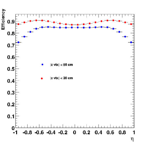
Figure 8.8: The $\pi^{-}$ reconstruction efficiency as a function of pseudorapidity. Two different vertex selections are shown, illustrating the influence of the choice of vertex on the efficiency due to the detector geometry.

The two data sets in the figure are for selections of events with vertex $z$ position, $z_{\mathrm{vertex}}$, within $\pm 95$ cm (blue points) and $\pm 20$ cm (red points) of the center of the TPC. The wide vertex cut allows us to use most of the available data. The interest in studying such variations in efficiency lies in the observation that a particular phase space region, for a given vertex position, will be measured in a different region of the detector. For example, tracks with $\eta$ > 0.5 will not cross all the available padrows in the TPC when the vertex is in a position $z_{\mathrm{vertex}}$ > 95 cm. This is reflected as a drop in the efficiency. By making a tighter $z_{\mathrm{vertex}}$ cut, one can probe a wider phase space region with the guarantee that tracks have the chance to cross all TPC padrows. For a vertex cut of |$z_{\mathrm{vertex}}$| < 20 cm, tracks within $|\eta|<0.8$ will cross the entire TPC, and one can see a higher efficiency for these tracks in the figure (red points).

Furthermore, even when tracks cross the entire TPC, we also expect a variation in efficiency for a given $\eta$ slice as a function of the vertex position. This arises from diffusion effects, as a track crossing the detector in the region near the central membrane will produce space points that must drift across the entire chamber, and their clusters will be wider than those for tracks near the pad plane. We can test the adequacy of our detector simulation by studying the raw and corrected yield in a given $\eta$ bin as a function of the vertex position, and hence as a function of the position of the track in the detector. In addition, since the TPC volume is separated into two identical halves separated at $z=0$ and set up such that the ionization drifts toward the wires (located at $\pm 2.1$ m), the behaviour for a given choice $\eta$ and $z_{\mathrm{vertex}}$ should be the same as for $-\eta$ and $-\mbox{$z_{\mathrm{vertex}}$}$. This is illustrated in Fig. 8.9 which shows the raw $\eta$ distribution for 10 cm slices in the choice of $z_{\mathrm{vertex}}$ interval: [20, 30] cm, [80, 90] cm; and the corresponding symmetric $z_{\mathrm{vertex}}$ selections [$-30$, $-20$] cm and [$-90$, $-80$] cm.

 

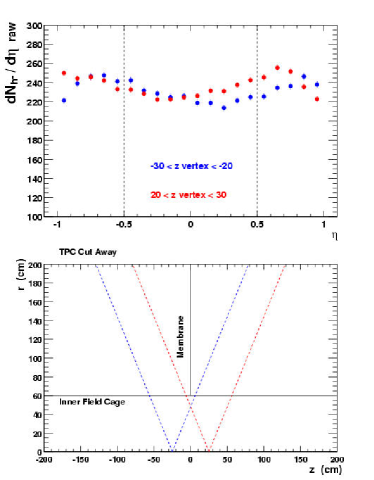
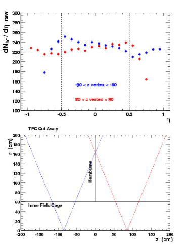
Figure 8.9: Raw yield dependence on $z_{\mathrm{vertex}}$. The left panel is for the vertex choice [20, 30] cm (red) and [$-30$, $-20$] cm (blue), right panel is for the interval [80, 90] cm (red) and [$-90$, $-80$] cm (blue). Dashed lines in the bottom panels represent tracks with $\eta=\pm 0.5$, corresponding to the limits given by the vertical dashed lines in the top panels.

The top panels show the raw distributions as a function of $\eta$, left for the [20, 30] cm interval and right for the [80, 90] cm region. In the bottom panel a sketch of the detector geometry is given, as a slice in the $r$ and $z$ coordinates of the TPC cylinder. The central membrane is at $z=0$, the drift distance is 2.1 m from the membrane to the wires. The first pad row at 60 cm and the last pad row at 200 cm. The lines in this panel represent the trajectories of tracks originating from the given vertex position at $\eta=\pm 0.5$. We can see that there are significant systematic variations in the raw yield depending upon where the event happened. As expected, the raw yield begins to decrease significantly once tracks do not cross the entire TPC. Such systematics must be taken into account in the efficiency corrections.

Since the corrected yield we report must be independent of any detector effects, it is easier to study the adequacy of the corrections by focusing on a single $\eta$ bin and comparing the raw and corrected yield for the bin as a function of the vertex position. This is illustrated in Fig. 8.10

 

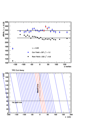
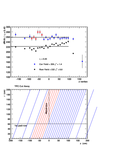
Figure 8.10: Raw and corrected yield for $-0.3<\eta<-0.2$ (left) and $0.4<\eta<0.5$(right) as a function of $z_{\mathrm{vertex}}$. Data points in each of the upper plots correspond to tracks crossing the detector region illustrated schematically in the lower plots.

which shows the raw and corrected yields for two choices of $\eta$, $-0.3<\eta<-0.2$ (left) and $0.4<\eta<0.5$ (right), as a function of $z_{\mathrm{vertex}}$. The lower panel shows the geometry of the relevant tracks as they cross the detector for the different vertex positions. The steps in $z_{\mathrm{vertex}}$ were done in 10 cm bin sizes between $\pm 100$ cm (20 bins), and 4 wider bins with limits $[-190,-140],\ [-140,-100],\ [100,140],\ [140,190]$ in order to get enough statistics (see the $z_{\mathrm{vertex}}$ distribution, Fig. 8.2). We again see that there are systematic effects in the raw yield. We can identify two general trends. For tracks that do not cross the entire TPC, the yield drops rapidly. For the remaining tracks, the raw yield is the lowest for tracks closest to the central membrane and increases as the tracks get closer to the pad planes on either side of the TPC. For reference, a fit to the raw data assuming a constant yield is done (black points) with a resulting poor $\chi^{2}$; 6.8 (left) and 8.8 (right). The corrected yield is essentially free of $z_{\mathrm{vertex}}$ systematics, except for two cases. In the events closest to the edges of the TPC, where the acceptance is varying rapidly and most of the tracks in the event lay outside the TPC, the tracks that do not cross the entire TPC show a corrected yield that is lower than the rest. This is expected, as tracks with very little information left in the detector will be difficult to reconstruct. We also found an additional systematic effect in the efficiency correction traced back to the simulation of tracks crossing the central membrane. This effect causes a slight over correction of the yield for such tracks, as can be seen by the corrected yield for these tracks which is coloured differently in the figure. Therefore, to prevent these systematic effects from appearing in the final pseudorapidity distribution, we included only events within $\pm 100$ cm of the center of the TPC, excluded tracks going through the membrane, and excluded tracks which did not cross the entire TPC. Each data point in the final $h^{-}$ pseudorapidity and $p_{\perp}$ distributions is then obtained as the average of each of the $\sim 20$ independent measurements of the corrected yield obtained for each of the $z_{\mathrm{vertex}}$ bins.

Since the most important correction for $p_{\perp}$ spectra and yields is the efficiency, this is where we concentrated a large fraction of the studies of systematic effects. The systematic uncertainty due to the corrections was estimated in two ways. In order to ensure consistency of the results, we studied the variation in the final spectra due to a large variation in the track quality cuts. The distributions of the cut variables are given in Fig. 8.11 from both data and simulations; the left panel shows the distance of closest approach distribution and the right panel shows the number of fit points distribution. We varied the selection based on number of fit points from 10 to 24 and the selection based on distance of closest approach from 3 cm to 1 cm. These choices are labelled “cut 1” and “cut 2” in the figure.

 

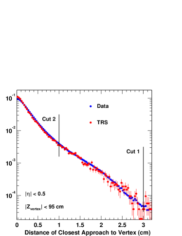
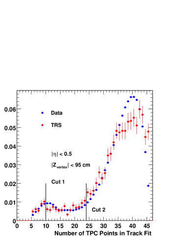
Figure 8.11: Comparisons of the distance of closest approach (a) and number of fit points (b) distributions for simulated and real data.

The different corrections for the more stringent set of cuts (cut 2) were then recalculated. The final multiplicity distribution obtained in both cases was compared and they were in agreement to $\sim 1\%$. To study the sensitivity to the cuts a small variation in the track quality cuts was then made, accepting tracks with 23 fit points. A corrected spectrum using the correction factors calculated for tracks with 24 fit points was then applied. This yields then a corrected distribution that is systematically higher than the measured value, as one is then over-correcting the raw data. The yield at high multiplicity obtained via this systematic effect was found to be 6.4% above the measured yield. This is the main contribution to the systematic uncertainty in the total particle yield for the analysis presented here.

8.2.3 Backgrounds

Instrumental backgrounds due to photon conversions and secondary interactions with detector material were estimated using the detector response simulations mentioned above, together with events generated by the hijing model [102, 103]. The simulations were calibrated using data in regions where background processes could be directly identified. The measured yield also contains contributions from the products of weak decays, primarily $K^{0}_{S}$, that were incorrectly reconstructed as primary tracks that must also be accounted for in the background correction. Figure 8.12 (left panel) illustrates

 

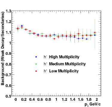
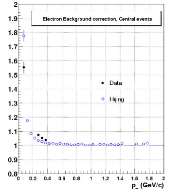
Figure 8.12: Background correction to the $h^{-}$ spectrum coming from weak decays and secondary interactions in the detector material (a) and electrons (b) as a function of $p_{\perp}$. The corrections were obtained via hijing events processed through the STAR offline simulation and reconstruction chain.

the background fraction of the raw signal coming from secondary interactions and decays. The shape of the background correction is independent of multiplicity. We see that the hadronic background is approximately 15% at $p_{\perp}$ = 100 $\mathrm{MeV/}c$, decreasing with increasing $p_{\perp}$ to a constant value of $\sim 7\%$. The average fraction of hadronic background tracks in the uncorrected sample is 7%. The error on the background correction increases with $p_{\perp}$ because statistics are limited, but there is also a systematic uncertainty associated with this correction. Since the background depends on the yields of various particles, in particular $K^{0}_{S}$ and $\bar{\Lambda}$, differences between the model and the data will systematically affect the correction. An estimate of the background correction at $p_{\perp}$ = 2 $\mathrm{GeV}$ assuming the ratios $\bar{\Lambda}/\mbox{$\bar{p}$}\sim 0.8$ and $\mbox{$\bar{p}$}/\mbox{$\pi^{-}$}\sim 1$ would yield a value of $\sim 1.15$ instead of $1.07$. This is the main source of systematic uncertainty in the hadronic background correction.

The right panel of Figure 8.12 shows the electron background obtained from $\frac{dE}{dx}$ data (filled points) and from hijing simulations (hollow points). The shape of the electron background is exponential, so we can use the shape and normalize to the data in order to obtain the final electron correction. Since the slope of the exponential can affect the final slope of the $p_{\perp}$ distribution, we can also do a correction using the hijing points to study the variation in the $p_{\perp}$ spectrum. We find that the choice of the slope in the electron correction changes the corrected value of $\langle p_{\perp}\rangle$ by 10 $\mathrm{MeV/}c$ and is the main contribution to the systematic uncertainty of the determination of $\langle p_{\perp}\rangle$.

8.2.4 Comparison of TPC Halves and Sector ($\phi$) Dependence

From the design of the TPC, the tracking volume is essentially divided into two independent halves and it is not a priori obvious that one can combine them without introducing systematic effects. Therefore, one of the necessary studies in the evaluation of the reliability of the results is to compare the raw yields in the different halves. However, one has to be careful in this comparison to isolate the possible differences. Because of the design of the TPC, we expect to see differences in the raw yields even within the same half of the TPC simply due to an increased drift length. As an example, we can take tracks close to midrapidity, which are emitted at an angle close to $90^{\circ}$. As the event vertex is not a fixed quantity in the z axis for the different events, tracks at midrapidity coming from events with different vertex z positions will have different drift distances, and thus we expect systematic differences in the raw yield at fixed $\eta$ for varying vertex z positions, as was discussed in Section  8.2.2. To isolate differences between the East ($z<0$) and West ($z>0$) halves of the TPC, we therefore have to make sure that we take event and track samples that are related by the transformation $\eta^{\mathrm{East}}=-\eta^{\mathrm{West}}$ and $z_{\mathrm{vertex}}^{\mathrm{East}}=-z_{\mathrm{vertex}}^{\mathrm{West}}$. In addition, as each TPC half is made up of 24 independent sectors to cover the full azimuthal range, it is also interesting to do a comparison of the raw azimuthal yields to make sure there are also no systematic effects. In doing this comparison, one can also separate the raw yields from positively and negatively charged tracks, for there might be distortions that affect these tracks differently. The tracks selected must also satisfy requirement of having at least 10 fit points (“cut 1” in Fig.8.11(b)). This cut is also used for the $h^{-}$ analysis.

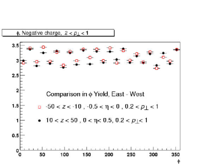
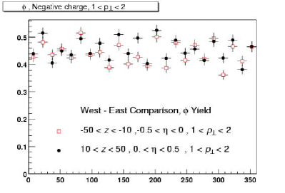
Figure 8.13: Raw $\phi$ distribution of East and West half of the TPC for negatively charged particles. Left panel: low $p_{\perp}$ (0.2 - 1 $\mathrm{GeV/}c$). Right panel: moderate $p_{\perp}$ (1 - 2 $\mathrm{GeV/}c$)

Figure 8.13 shows the raw azimuthal distribution for negatively charged tracks in the two halves of the TPC. The East half track sample, shown as the hollow square data points, was obtained from events with $-50<z_{\mathrm{vertex}}<-10$ cm and from tracks with $-0.5<\eta<0$. Similarly, for the West half the events had a vertex selection of $10<z_{\mathrm{vertex}}<50$ cm and tracks were selected according to $0<\eta<0.5$. The left panel shows the yields for the low $p_{\perp}$ region, 0.2 < $p_{\perp}$ < 1 $\mathrm{GeV/}c$. A similar plot showing the raw azimuthal distribution in the range 1 < $p_{\perp}$ < 2 $\mathrm{GeV/}c$ is shown in the right panel. The samples are normalized per event to isolate the differences in the raw yields.

The size of the bins in the azimuthal direction is $15^{\circ}$, or half a sector. We see that there is a periodic structure to the distribution in both cases. This comes about because charged tracks will curve in the magnetic field. Therefore, depending upon their charge sign and entrance point to a sector (i.e. their azimuthal angle), will have a trajectory that is either fully contained in a sector boundary or that crosses a sector boundary. For a specific charge sign, tracks in one side of the sector will be more easily reconstructed than on the other side, giving the structure seen in Figure 8.13. This effect is more pronounced for low momentum (i.e. large curvature) tracks. The high yield bins for the negative charge tracks should be the low yield bins for the positive ones. The low momentum positively charged tracks are shown in Figure 8.14. Indeed we see the expected change, for this case the first bin is a high yield bin (compare to Fig. 8.13).

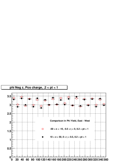
Figure 8.14: Raw $\phi$ distribution of East and West half of the TPC for low transverse momentum (0.2 - 1 $\mathrm{GeV/}c$) positively charged particles.

To focus on changes between East and West halves of the TPC, we make a ratio of the previous histograms. Figure 8.15 shows the ratio for low $p_{\perp}$ negative (a) and positive (b) tracks. The average difference in both cases is on the order of 1%.

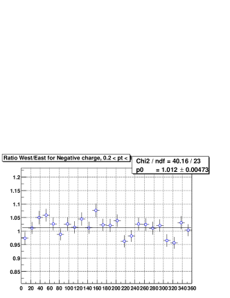
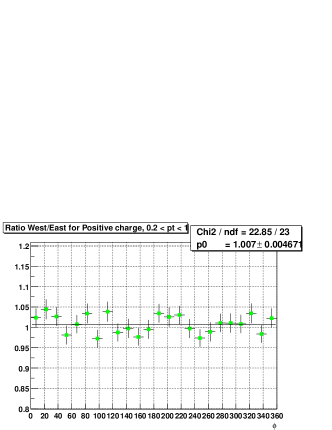
Figure 8.15: Ratio of raw $\phi$ distribution of East and West half of the TPC for low transverse momentum (0.2 - 1 $\mathrm{GeV/}c$) negatively (a) and positively (b) charged particles.

We can also make a comparison of the $\mbox{$h^{-}$}/\mbox{$h^{+}$}$ ratio in both halves of the TPC. Since we know that there will be systematic differences as a function of $\phi$ due to the curvature effect mentioned before, we can simply make a ratio of the raw yields integrated over $\phi$. For the East half of the TPC we find $\mbox{$h^{-}$}/\mbox{$h^{+}$}=0.983\pm 0.005$ and for the West half a similar analysis yields $\mbox{$h^{-}$}/\mbox{$h^{+}$}=0.988\pm 0.005$ where the errors are statistical only. We conclude that for the purposes of this analysis the two halves of the TPC yield sufficiently similar results.

However, we will still separate the corrections to the raw yields in other variables as mentioned in Sec. 8.2.2. We expect variations in the raw yields due to different track geometries and event topology. In summary, we expect that tracks that do not cross the entire tracking volume of the TPC to be more difficult to reconstruct than those tracks that do. In addition, it is much easier to reconstruct the tracks when there are not many tracks in the detector, so we must see a decrease in the tracking efficiency in a high multiplicity environment. Furthermore, low momentum tracks coming from the interaction vertex will have a difficult time reaching the tracking volume. The radial distance at the center of the first TPC sensitive pad row is 60 cm, which along with the magnetic field of 0.25 T places an effective low $p_{\perp}$ acceptance cut-off for primary tracks of $\sim 50\ \mbox{$\mathrm{MeV/}c$}$. Finally, as mentioned before even tracks in identical regions of phase-space will have different raw yields depending upon where the event vertex was placed because they will sample a different detector geometry. Therefore, we have divided all the tracking corrections according to

• the phase-space cell occupied by the tracks,

• the multiplicity of the event, and

• the position of the primary vertex.

The previous corrections are the most important ones in the present analysis. The following corrections to the spectra and yields were also studied. Each of them was found to produce changes of less than 1%.

8.2.5 Momentum resolution

The momentum resolution is momentum dependent. It is well known that for a $p_{\perp}$ distribution, the resolution of the detector will introduce a change in the slope of the observed spectrum. This can be seen from the following simple argument. The effect of a finite momentum resolution is that a certain number of tracks will be reconstructed with the wrong momentum, and will therefore be counted in an incorrect bin. It is possible for a track to be reconstructed with a lower or a higher $p_{\perp}$. So for a given $p_{\perp}$ bin, there will be a loss of particles to adjacent bins and a gain of particles from adjacent bins. The magnitudes of these fluxes compared to the yield in the given bin are the important quantities. From the rapid decrease in cross section with increasing $p_{\perp}$, we expect that the feeding of particles from the lower to the higher $p_{\perp}$ bins will be higher than the flux in the opposite direction, and hence the net effect is to flatten the spectrum to some extent. This effect becomes important when the momentum resolution is of the same order as the size of the $p_{\perp}$ bin. It is therefore necessary to quantify this effect in any momentum analysis.

For the results presented here we concentrate on $\mbox{$p_{\perp}$}\leq 2$ $\mathrm{GeV/}c$. We find the momentum resolution to be better than 4% as illustrated in Fig. 6.6. For a $p_{\perp}$ bin width of 100 $\mathrm{MeV/}c$ we expect the correction due to momentum resolution to be less than 1% in the full range of $p_{\perp}$. This effect was quantified in two different analyses. The first approach relies on the embedding procedure, and consists of dividing the phase space into bins and using the track matching between simulated and reconstructed tracks from. We can keep track of the $p_{\perp}$ bin in which a particle was created, and then see if it was reconstructed in the same bin. We can thus know, for each phase space bin, what percent of tracks are reconstructed correctly, what percent are reconstructed in a different bins and correct for the resolution.

The only significant correction found this way occurs for the very first $p_{\perp}$ bin. The reason is the following. The raw yield in each bin is composed of two parts: the tracks which were correctly reconstructed in the same $p_{\perp}$ bin as the one they were generated in, let’s call these the healthy tracks; and the tracks that are found by the reconstruction but placed in a different bin than the one they were generated in, let’s call these the crippled tracks. Now let’s focus on the region $\mbox{$p_{\perp}$}<100\ \mbox{$\mathrm{MeV/}c$}$ where the efficiency drops very rapidly with decreasing $p_{\perp}$. There will be very few healthy tracks in the first $p_{\perp}$ bin because the efficiency is low. There will be, however, a considerable amount of crippled tracks in the first bin coming from the feed-down from the next (high efficiency) $p_{\perp}$ bins. The crippled tracks are almost as numerous as the healthy population for this bin. We therefore must apply a correction to obtain a realistic estimate of the initial healthy population in that bin. For the region $\mbox{$p_{\perp}$}>200\ \mbox{$\mathrm{MeV/}c$}$ the efficiency is independent of $p_{\perp}$ so we need only concentrate on the $p_{\perp}$ dependence of the parent distribution which we want to measure.

We can also calculate the expected correction based on a knowledge of the momentum resolution, the bin size, and a given $p_{\perp}$ distribution. One way to treat this problem is through an iterative procedure, starting with a given input $p_{\perp}$ distribution, doing a Monte Carlo study by smearing the tracks with the measured $p_{\perp}$ resolution and looking at the shape of the resulting distribution. We repeat the process until the output distribution matches the one measured in the experiment. The approach we followed relies on a related method. Starting from a given input $p_{\perp}$ distribution we use the measured $p_{\perp}$ resolution as a function of $p_{\perp}$ to construct a set of Gaussians (one for each $p_{\perp}$ bin). We also used different functional forms to parameterize the shape of the $p_{\perp}$ resolution, e.g. Lorenzian and double-Gaussian, yielding similar results. The area under each Gaussian is the initial yield for each $p_{\perp}$ bin, the mean is the center of the $p_{\perp}$ bin and the $\sigma$ is obtained from the measured $\delta\mbox{$p_{\perp}$}$ vs. $p_{\perp}$ curve. We can then figure out what is the contribution of each $p_{\perp}$ bin to any other bin in principle. In practice, each bin only contributes mainly to its nearest and next-to-nearest neighbours. The observed yield in the $i^{\mathrm{th}}$ $p_{\perp}$ bin, $N_{i}^{\mathrm{obs}}$ is then:

$$N_{i}^{\mathrm{obs}}=\sum_{k=0}^{\infty}N_{k}\int_{p_{\perp}(i)}\frac{1}{\sqrt{2\pi}\sigma_{k}}e^{\frac{(p_{\perp}-p_{\perp}(k))^{2}}{2\sigma_{k}^{2}}}dp_{\perp}$$ (8.3)

We can think of Eq. 8.3 as defining a matrix equation

$$N_{i}^{\mathrm{obs}}=\sum_{k=0}^{\infty}N_{k}C_{ki}$$ (8.4)

where the elements of the matrix $C_{ki}$ are defined by the integral of Eq. 8.3, and are interpreted as the percent contribution of bin $k$ to bin $i$, i.e. the mean of the Gaussian is the center of bin $k$ and the integration limits are given by the upper and lower limits of the $i^{\mathrm{th}}$ $p_{\perp}$ bin. The width of the Gaussian is given by the detector resolution at $p_{\perp}$ bin $k$. Therefore, the integral depends only on quantities that are measurable (the resolution) or defined by our analysis (the bin limits and bin center). This matrix then embodies all our knowledge of the effects of resolution.

For a given $p_{\perp}$ distribution, we can then calculate what the observed distribution will be and obtain appropriate correction factors for the effect of resolution. We have performed this procedure with different input distributions – power-law function, exponential in $p_{\perp}$ and exponential in $m_{\perp}$ with various slope parameters – and find that in all cases the correction for any given $p_{\perp}$ bin is less than 1% in the range up to 2 $\mathrm{GeV/}c$ with our given bin size. This is true for both the $h^{-}$/$h^{+}$ analysis (bin size 100 $\mathrm{MeV/}c$, range 0.1 - 2 $\mathrm{GeV/}c$) and for the $\pi^{-}$ analysis (bin size 50 $\mathrm{MeV/}c$, range 0.05 - 0.75 $\mathrm{GeV/}c$). For higher $p_{\perp}$ the resolution plays a more significant role, where we expect a correction of 20% or more at   5 $\mathrm{GeV/}c$ with a 1 $\mathrm{GeV/}c$ bin size and the present magnetic field of $B=0.25$ T.

An additional advantage of this resolution study is that, once we construct the $C_{ki}$ resolution matrix, we can also use it to recover the original yields $N_{k}$ by inverting the matrix, and no iterative procedure is needed:

$$N_{k}=\sum_{i=0}^{\infty}N_{i}^{\mathrm{obs}}(C_{ki})^{-1}$$ (8.5)

8.2.6 Track splitting

For a loose track selection based on the number of points reconstructed in the TPC, it is possible to overestimate the track yield in the presence of split tracks. This effect can come about for example when the track-finding algorithm fails to recognize two track segments as belonging to a single particle. This can happen typically when there are gaps in the track pattern, such as tracks crossing sector boundaries, tracks crossing the central membrane of the TPC, or tracks crossing a region of the TPC where the read out pad is noisy or dead.

To study the effect of splitting in this analysis, we used two approaches that relied on the detector simulation. An additional study was made using only real reconstructed tracks. All three results are in agreement both in the size of the overall effect and on its $p_{\perp}$ dependence. We will discuss the approach that relies on full simulation, since this is the most straight-forward.

In a full Monte Carlo generated event, we have all the information about the input tracks. Running the tracks through the GEANT implementation of the STAR detector, we obtain among other things the information on the TPC energy deposition left by the tracks. This is the input to the microscopic simulation of the TPC response yielding as output a simulated raw-data file that is then passed through the STAR reconstruction chain. A comparison of the TPC space points that are found by the reconstruction algorithms to the GEANT input is then performed. As discussed in Section 7.5, the matching as implemented in this analysis is based on spatial proximity. A feature of this matching procedure is that it allows a many-to-many matching: if 2 hits are very close together for example there will be a 2-to-2 hit match. Each of the 2 Monte Carlo hits will be matched to the 2 reconstructed hits.

The match of simulated point to reconstructed point serves as the footing for a simulated track to reconstructed track association. Typically, the association is 1-to-1. A split track will have a different topology. There will be one original Monte Carlo track, but it will be associated to 2 (or more) reconstructed tracks. The association algorithm allows a many-to-many type of matching, so one must be careful to really single out a split track from other matching topologies. We look for a single Monte Carlo track matched to more than one reconstructed track, and those reconstructed tracks are singly matched to the Monte Carlo track. Through this procedure, an estimate of the split track population and was found to be also below the 1% level. In addition, the analysis done with the more stringent requirement on the number of fit points (“cut 2” in Fig. 8.11(b)) guaranteed that there are is no double counting from split tracks. The results obtained from both analyses were found to be consistent.

8.2.7 Track merging

When 2 tracks lie very close together, the cluster finder might not be able to resolve the 2 ionization peaks and produce a single space point when there were originally 2 for each hit in the track trajectory. The losses due to this effect were estimated to be less than 1% for the most central collisions and negligible for peripheral collisions.

8.2.8 Ghost Tracks

This correction takes into account possible cases where the track finding algorithm might associate space-points from different tracks and give us track parameters from a non-existent particle. It was not known if this could be of importance in the high multiplicity environment of a heavy ion collision at high energy. It was found that the TPC occupancy was low enough that this did not present a problem. Essentially no such tracks were found in all the simulation and embedding analyses even at higher simulated multiplicities than those observed in the data.

Finally, all analyses were carried out with 3 different software production versions. As we understood the systematics of the detector better, we incorporated our knowledge of the calibrations, distortions and corrections to software bugs. The first production was done in August while data was still being taken. This was followed almost immediately by a new production one month later with improved calibrations. The data presented here is produced with the calibrations and distortion corrections processed in early 2001. The biggest systematic effect observed throughout this process was a 4.5% change in the efficiency obtained from the first simulations compared to the following two software versions. This was understood as coming from a more realistic parameterization of the allowed space point errors used during the track finding algorithm based on the measured residuals obtained in the first analysis of the data.

Chapter 9 Results and Discussion: Charged Hadrons

9.1 Multiplicity Distribution

9.1.1 Results

Figure 9.1 shows the corrected, normalized multiplicity distribution within $|\eta|<0.5$ and $\mbox{$p_{\perp}$}>100\ \mbox{$\mathrm{MeV/}c$}$ for minimum bias $\mathrm{Au}+\mathrm{Au}$ collisions. For this plot, a total of 350K minimum bias triggers were analyzed, yielding 119,205 events with a reconstructed vertex in the region |$z_{\mathrm{vertex}}$| < 95 cm.

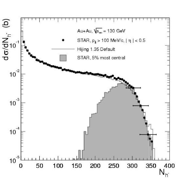
Figure 9.1: Normalized multiplicity distribution of $h^{-}$ with $\mbox{$p_{\perp}$}>100\ \mbox{$\mathrm{MeV/}c$}$, $|\eta|<0.5$ in $\mathrm{Au}+\mathrm{Au}$ collisions at $\mbox{$\sqrt{s_{{}_{\mathrm{NN}}}}$}\,=130\ \mbox{$\mathrm{GeV}$}$. The shaded area is 5% most central collisions, selected by ZDC signal (see text). The solid curve is the prediction from the hijing model.

The distribution for the 5% most central collisions (360 mbarn), defined using ZDC coincidence, is shown as the shaded area in Fig. 9.1. The definition adopted here was based on the signals shown in Fig. 8.1, by selecting events with ZDC sum $<66$ ADC counts and a high CTB threshold placed at 8500 ADC counts to remove the ambiguity between central and peripheral collisions. The actual value of the ZDC sum threshold is set by requiring the shaded area in Fig. 9.1 to equal 5% of $\sigma_{\mathrm{AuAu}}$. This is the event selection that was used for the $h^{-}$ $p_{\perp}$ and $\eta$ distributions for central events presented in the following sections.

The data were normalized assuming a total hadronic inelastic cross section of 7.2 barn for $\mathrm{Au}+\mathrm{Au}$ collisions at $\mbox{$\sqrt{s_{{}_{\mathrm{NN}}}}$}\,=130\ \mbox{$\mathrm{GeV}$}$, derived from Glauber model calculations. The first bin (below $N_{h^{-}}$ = 5) is not shown, due to systematic uncertainties in the vertex reconstruction efficiency and background contamination. Its relative contribution to the total cross section was estimated to be 21% by normalizing the hijing multiplicity distribution to the measured data in the region $5<\mbox{$N_{h^{-}}$}<25$ (i.e. the first three bins of Fig. 9.1). This procedure relies on the assumption that very peripheral interactions are well described by the superposition of a few nucleon-nucleon collisions in the geometry of a nuclear collision, and can therefore be accurately modelled by hijing. A comparison of the actual yield measured in the first bin (after the efficiency correction) to the shape predicted by the hijing model indicates a relative difference of 10%. The systematic uncertainty on the vertical scale is therefore estimated to be $\sim 10\%$ and is dominated by uncertainties in the total hadronic cross section and the relative contribution of the first bin. The systematic uncertainty on the horizontal scale is 6.4% for the entire range of multiplicity and is depicted by horizontal error bars on 3 data points only to maintain clarity in the figure.

The shape of the $h^{-}$ multiplicity distribution is dominated over much of the $N_{h^{-}}$ range by the nucleus-nucleus collision geometry, consistent with findings from lighter systems and lower energies. However, the shape of the tail region at large $N_{h^{-}}$ is determined by fluctuations and detector acceptance. These overall features are also observed in the hijing calculation, shown as histogram in Fig. 9.1 (although a more detailed comparison indicates that, for the model, the shape of the tail shows a different contribution due to fluctuations than that found in the data).

9.1.2 Discussion

The negatively charged particle multiplicity distribution reveals that the bulk features of the dynamics are dominated by the geometry. The shape shows the same features expected from a Glauber picture of a superposition of nucleon-nucleon collisions. The model proposed by Kharzeev and Nardi [93] attempts to extract the contribution to the multiplicity distribution that scales as either soft or hard processes, or more precisely, as $N_{\mathrm{part}}$ and $N_{\mathrm{coll}}$. Such scaling is expected to be $p_{\perp}$ dependent, and therefore this study is better suited for a $p_{\perp}$ distribution (see Sec. 9.2).

It is nevertheless useful to apply such models in order to obtain a statistical determination of the number of participants for a given event selection. One implementation of the Glauber particle production model is illustrated in Fig. 9.2.

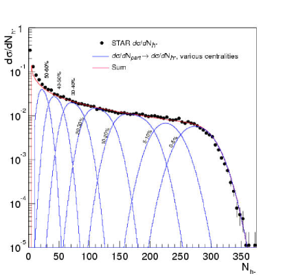
Figure 9.2: Fit to the multiplicity distribution $d\sigma/dN_{h^{-}}$ using a Glauber model (Sec. 4.1.1)

.

This was done by a Monte Carlo implementation, where one generates events with random impact parameter, and then samples the $d\sigma/db$ geometrical distribution to find the probability to have an event at the given impact parameter. When an interaction takes place, we calculate $N_{\mathrm{part}}$ and $N_{\mathrm{coll}}$ using Eq.4.9. We can thus obtain a $d\sigma/d\mbox{$N_{\mathrm{part}}$}$ distribution which we use as a weight in the final multiplicity distribution (similar to the weight in Eq. 4.13 given by the probability of no interaction). We can assume that particle production is proportional to the number of participants (Sec. 4.1.1) $\langle\mbox{$N_{h^{-}}$}(b)\rangle=q\langle\mbox{$N_{\mathrm{part}}$}(b)\rangle$, or use a linear combination of $N_{\mathrm{part}}$ and $N_{\mathrm{coll}}$  à la Kharzeev-Nardi [93] (Eq. 4.10). As mentioned before, we also choose Gaussian fluctuations, Eq. 4.12. The approach works best from mid-central to central collisions, as the fluctuations in peripheral collisions are large. Figure 9.2 shows the result of applying such a model to the STAR multiplicity distribution. The blue curves are the distributions obtained by binning the $d\sigma/d\mbox{$N_{\mathrm{part}}$}$ distribution to get successively $0-5\%$, $5-10\%$, $10-20\%$, $20-30\%$, $30-40\%$, $40-50\%$, and $50-60\%$ of $\sigma_{\mathrm{AuAu}}$, which result in the blue curves with near-Gaussian tails when transformed to $d\sigma/dN_{h^{-}}$ because of the fluctuations. The red curve is the convolution of all such distributions, giving a fit to the multiplicity distribution. The size of the fluctuations in Eq. 4.12 is found to be $a=1.45\pm 0.2$. This parameter is constrained mostly by the shape of the terminus of the distribution. For a Poisson distribution, this value would be 1. The presence of correlations makes this value exceed unity. The origin of the correlations from the dynamics of the colliding system is a combination of nucleus-nucleus geometry fluctuations, nucleon-nucleon cross section fluctuations and hadron resonance correlations [151]. In fact, this parameter for hijing turns out to be rather large, $a\gtrsim 4$, as is also apparent in Fig.9.1. There are also fluctuations due to finite detector acceptance. Since the TPC has a large acceptance, the contribution from acceptance fluctuations is small. The shape of the terminus of the distribution measured with a smaller acceptance apparatus should be reveal a less steep shape of the terminus of the distribution (i.e. a larger $a$), e.g. the PHENIX Pad Chamber measurement [152].

It is argued [153] that the centrality dependence of the rapidity density per participant pair can distinguish between models based on particle production from gluon saturation (EKRT [154]) from those based on fixed scale pQCD such as hijing. In the EKRT model, particle production is computed assuming that the pQCD growth of low $p_{\perp}$ gluons is only integrated up to a certain saturation scale. The saturation requirement has as a consequence that the multiplicity per participant decreases with centrality. For hijing, particle production arises from two main contributions: (a) a component arising from low-$p_{\perp}$ hadron production, modelled as beam jet string fragmentation, which is essentially proportional to $N_{\mathrm{part}}$, and (b) a contribution arising from mini-jet production, which is directly proportional to $N_{\mathrm{coll}}$ and to the averaged inclusive jet cross section per nucleon-nucleon collision. This is essentially the same functional dependence as Eq. 4.10. The centrality dependence of the mid-rapidity density for hijing is then

$$\frac{dN_{\mathrm{ch}}}{d\eta}=\langle\mbox{$N_{\mathrm{part}}$}\rangle n_{\mathrm{soft}}+f\langle\mbox{$N_{\mathrm{coll}}$}\rangle\frac{\sigma_{\mathrm{jet}}^{A}A(\mbox{$\sqrt{s}$})}{\sigma_{in}^{NN}}$$ (9.1)

where $n_{\mathrm{soft}}\approx 1.3$ and $f\approx 1.2$. A plot of $dN/d\eta/(\mbox{$N_{\mathrm{part}}$}/2)$ vs. $N_{\mathrm{part}}$ should then naïvely grow as $\sim\mbox{$N_{\mathrm{part}}$}^{1/3}$. Using the Monte Carlo model just discussed, and also the model from Kharzeev and Nardi [93] applied to the STAR data, we obtain the centrality dependence of $dN/d\eta$ shown in Fig. 9.3.

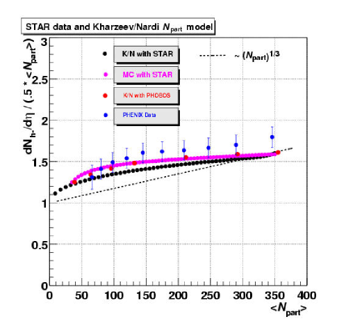
Figure 9.3: $dN/d\eta$ per participant pair vs. $N_{\mathrm{part}}$.

The results from PHENIX [152] and from the Kharzeev and Nardi analysis of the PHOBOS results  [93] are also shown. The growth with $N_{\mathrm{part}}$ clearly disfavours the saturation picture from Ref.[154]. As pointed out in Ref.[93], the original saturation ideas pertain to the behaviour of partons in the initial wave function of the nucleus; and when taking this approach the predictions surprisingly turn out to be quite similar to the eikonal Glauber approach discussed in Sec. 4.1.1. There are also deviations from the simple $\mbox{$N_{\mathrm{part}}$}^{1/3}$ dependence which can arise from the dilute edges of the Wood-Saxon nuclear distribution (Fig. 4.1) and from other medium effects such as nuclear shadowing of the initial parton distributions [155] or jet quenching[76, 77]. The similarity between the conventional approach and the high-density QCD approach makes it difficult to distinguish which underlying picture is correct. These effects are therefore better studied in the differential $p_{\perp}$ distributions.

9.2 $p_{\perp}$ Distribution

9.2.1 Results

Since the yield of charged hadrons at midrapidity depends on the extrapolation of the $p_{\perp}$ distribution outside the measured range, we discuss the $p_{\perp}$ spectrum first. The shape of the $p_{\perp}$ distribution is well suited for more detailed scrutiny. Figure 9.4 shows the $p_{\perp}$ distribution for positively and negatively charged hadrons ($h^{+}$ and $h^{-}$).

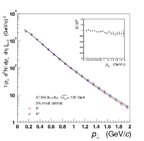
Figure 9.4: The $p_{\perp}$ distributions for $h^{-}$ (open circles) and $h^{+}$ (open “plus” sign) in central collisions. The inset shows the ratio $\mbox{$h^{-}$}/\mbox{$h^{+}$}$ vs. $p_{\perp}$. The data are fit to a power law in $m_{\perp}$ to obtain the extrapolated yield $dN/d\eta$ (see text).

Statistical errors are smaller than the symbols. The correlated systematic uncertainty is estimated to be below 6%. The $p_{\perp}$ distributions in this range of centre-of-mass energies are customarily fit by a QCD inspired power-law function of the form $d^{2}\mbox{$N_{h^{-}}$}/dp_{\perp}^{2}d\eta=A\,(1+\mbox{$p_{\perp}$}/p_{0})^{-n}$ where $A$, $n$, and $p_{0}$ are free parameters. This power-law fit is useful in comparison to other reference data such as $p_{\perp}$ spectra from $p\bar{p}$ collisions [96]. For the extrapolation to $p_{\perp}$ = 0, it is better to use a modified version of the power law, and use $m_{\perp}$ instead of $p_{\perp}$ in order to better reproduce the data at low $p_{\perp}$. This is the fit shown in Fig. 9.4, using a mass slightly larger than the $\pi^{-}$ mass, since the $h^{-}$ spectrum is made not only of pions but includes $K^{-}$ and $\bar{p}$ as well. The “mean mass” of the $h^{-}$ distribution must therefore be $\langle m\rangle\gtrsim m_{\pi}$. We studied the effect that such variations in the shape of the extrapolating function have on the yield by comparing the $m_{\perp}$ and $p_{\perp}$ power-law fits and also a simple exponential fit at low $p_{\perp}$. The yield in the region $0-100\ \mbox{$\mathrm{MeV/}c$}$ was found to be $6.8\%$ using the $m_{\perp}$ power law, the other fits varied from this by about $\pm 1.5\%$ which we take as an additional systematic uncertainty for the extrapolated yield. The choice of mean mass does not influence the extrapolated yield obtained from the $m_{\perp}$ power law, it was found to vary less than 0.5% with mean masses in the range $140-200\ \mbox{$\mathrm{MeV/}c^{2}$}$. The $\chi^{2}/\mathrm{\textit{d.o.f.}}$ was minimized with a value of $\langle m\rangle\simeq 187\ \mbox{$\mathrm{MeV/}c^{2}$}$. In all cases, the yield in the region $\mbox{$p_{\perp}$}>2\ \mbox{$\mathrm{GeV/}c$}$ was $\lesssim 1\%$. We therefore use an extrapolation factor of $7\pm 1.5\%$ to obtain $dN/d\eta$.

9.2.2 Discussion

We focus now on the comparison of the measured $p_{\perp}$ spectrum in $\mathrm{Au}+\mathrm{Au}$ at RHIC to other energies and collision systems. We will focus more on $p\bar{p}$ collisions. Figure 9.5, upper panel, shows the transverse momentum distribution of negatively charged hadrons for central $\mathrm{Au}+\mathrm{Au}$ collisions at mid-rapidity ($|\eta|<0.1$) within $0.1<\mbox{$p_{\perp}$}<2\ \mbox{$\mathrm{GeV/}c$}$.

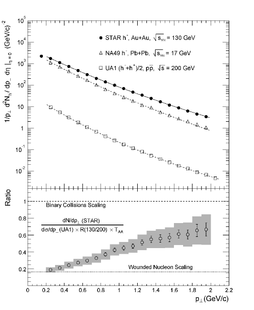
Figure 9.5: Upper panel: $h^{-}$ $p_{\perp}$-spectra for the 5% most central $\mathrm{Au}+\mathrm{Au}$ collisions at mid-rapidity ($|\eta|<0.1$). Central $\mathrm{Pb}+\mathrm{Pb}$ data from NA49 at lower energy and $p\bar{p}$ data from UA1 at a similar energy are also shown. The curves are power-law fits to the data. Lower panel: ratio of STAR and scaled UA1 $p_{\perp}$-distributions (see text).

The upper panel of Fig. 9.5 also shows the $p_{\perp}$-distributions of negatively charged hadrons for central $\mathrm{Pb}+\mathrm{Pb}$ collisions at $\sqrt{s_{{}_{\mathrm{NN}}}}$ = 17 $\mathrm{GeV}$ from NA49 [105] and for minimum-bias $p\bar{p}$ collisions at $\sqrt{s}$ = 200 $\mathrm{GeV}$ from UA1 [96], fitted with the same function. The NA49 distribution, which was reported in units of pion rapidity, was transformed to units of pseudorapidity. The UA1 invariant cross section $Ed^{3}\sigma/d^{3}p$ reported in Ref. [96] was scaled by $2\pi/\mbox{$\sigma_{\mathrm{inel}}$}$, where $\mbox{$\sigma_{\mathrm{inel}}$}=42$ mb for $\sqrt{s}$ = 200 $\mathrm{GeV}$ [95]. The power law fits all three datasets well. The mean $p_{\perp}$ can be derived from the fit parameters as $\mbox{$\langle p_{\perp}\rangle$}=2p_{0}/(n-3)$. The fit to the STAR data gives $p_{0}=3.0\pm 0.3\ \mbox{$\mathrm{GeV/}c$}$, $n=14.8\pm 1.2$, and $\mbox{$\langle p_{\perp}\rangle$}=0.508\pm 0.012\ \mbox{$\mathrm{GeV/}c$}$. The strong correlation of fit parameters $p_{0}$ and $n$ must be taken into account when calculating the error on $\langle p_{\perp}\rangle$. The $\langle p_{\perp}\rangle$ from STAR is larger than that from both central collisions of heavy nuclei at much lower energy ($\mbox{$\langle p_{\perp}\rangle$}_{\mathrm{NA49}}=0.429\ \mbox{$\mathrm{GeV/}c$}$) and nucleon-nucleon collisions at a comparable energy ($\mbox{$\langle p_{\perp}\rangle$}_{\mathrm{UA1}}=0.392\ \mbox{$\mathrm{GeV/}c$}$).

Figure 9.5, lower panel, shows the ratio of the STAR and UA1 $p_{\perp}$-distributions. Since the UA1 distribution is measured at $\sqrt{s}$ = 200 $\mathrm{GeV}$, $d\sigma/d\mbox{$p_{\perp}$}$ is scaled by two factors for quantitative comparison to the STAR data at 130 $\mathrm{GeV}$: (i) $R(130/200)$, the $p_{\perp}$-dependent ratio of invariant cross sections for charged particle production in $p\bar{p}$ collisions at $\sqrt{s}$ = 130 and 200 $\mathrm{GeV}$, and (ii) $\mathrm{T}_{\mathrm{AA}}$= $26\pm 2$ mb^-1, the nuclear overlap integral [28] for the 5% most central $\mathrm{Au}+\mathrm{Au}$ collisions. $R$ varies from 0.92 at $\mbox{$p_{\perp}$}=0.2\ \mbox{$\mathrm{GeV/}c$}$ to 0.70 at $\mbox{$p_{\perp}$}=2.0\ \mbox{$\mathrm{GeV/}c$}$, and was derived using scaling laws for $\langle p_{\perp}\rangle$ and $dN_{\mathrm{ch}}/d\eta$ as a function of $\sqrt{s}$ [96, 39] together with the extrapolation to 130 $\mathrm{GeV}$of power-law parameterizations at $\sqrt{s}$ = 200–900 $\mathrm{GeV}$[96]. The shaded boxes show the total error of the ratio, which is the linear sum of the errors of the measured data, depicted by the error bars, and the systematic uncertainty due to uncertainties in the scaling with $\mathrm{T}_{\mathrm{AA}}$ and $R$.

There are two simple predictions for the scaled ratio. In lower energy hadronic and nuclear collisions, the total pion yield due to soft (low $p_{\perp}$) processes scales as the number of participants (or “wounded” nucleons) in the collision (see e.g. Ref.  [31, 105]). The scaled ratio in this case is 0.164, assuming 172 participant pairs and a mean number of binary collisions of 1050 ($=\mbox{$\sigma_{\mathrm{inel}}$}\,\mbox{$\mathrm{T}_{\mathrm{AA}}$}$, $\mbox{$\sigma_{\mathrm{inel}}$}\ =40.35$ mb) for the 5% most central $\mathrm{Au}+\mathrm{Au}$ events (Sec. 4.1.1). In contrast, if hadron production is due to hard (high $p_{\perp}$) processes and there are no nuclear-specific effects, the hadron yield will scale as the number of binary nucleon-nucleon interactions in the nuclear collision and the value of the ratio is unity. There are important nuclear effects which will alter the scaling as a function of $p_{\perp}$ from these simple predictions, including initial state multiple scattering [121], shadowing [155], jet quenching [76, 77], and radial flow [156]. The scaled ratio exhibits a strong $p_{\perp}$ dependence, rising monotonically with increasing $p_{\perp}$ from Wounded Nucleon scaling at low $p_{\perp}$ but not reaching Binary Collision scaling at the highest $p_{\perp}$ reported. This is consistent with the presence of radial flow, as well as the onset of hard scattering contributions and initial state multiple scattering with rising $p_{\perp}$. From $pA$ collisions at lower energy, the data tend to show an increase beyond the scaling with binary collisions. This “Cronin” effect is thought to arise from initial state multiple scattering in the nuclear medium, which broadens the $p_{\perp}$ spectrum [121]. At SPS, the $p_{\perp}$ spectra indicate a similar increase beyond binary collision scaling for the region $\mbox{$p_{\perp}$}\sim 2\ \mbox{$\mathrm{GeV/}c$}$. Although a comparison of the $p_{\perp}$ dependence of the data at different $\sqrt{s_{{}_{\mathrm{NN}}}}$ is better done in $x_{\perp}=2\mbox{$p_{\perp}$}/\mbox{$\sqrt{s}$}$ rather than in $p_{\perp}$, there are indications from preliminary STAR[91] and PHENIX [157] hadron spectra at high $p_{\perp}$that the scaling with $N_{\mathrm{coll}}$ is not reached even for $p_{\perp}$ 2 - 6 $\mathrm{GeV/}c$. This effect has sparked active discussions in the community vis-à-vis the possibility of being related to parton energy loss in a QGP, i.e. jet quenching [158].

9.3 $\eta$ Distribution

9.3.1 Results

By integrating the $p_{\perp}$ spectra for different $\eta$ bins, we obtain the $dN/d\eta$ vs. $\eta$ distribution. Figure 9.6 shows the normalized pseudorapidity distribution of $h^{-}$ and $h^{+}$ for the 5% most central collisions within $|\eta|<1.0$. The black points are the measured yield for $0.1<\mbox{$p_{\perp}$}\ <2\ \mbox{$\mathrm{GeV/}c$}$ and the hollow points are the extrapolation for all $p_{\perp}$.

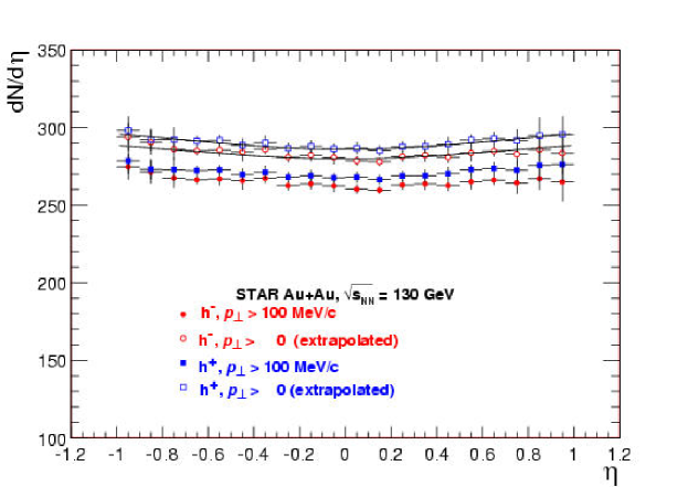
Figure 9.6: $h^{-}$ (red circles) and $h^{+}$ (blue squared) pseudorapidity distribution from 5% most central $\mathrm{Au}+\mathrm{Au}$ collisions. Data are integrated over $\mbox{$p_{\perp}$}\,>100$ $\mathrm{MeV/}c$ (filled symbols), and extrapolated to all $p_{\perp}$ (open symbols).

The latter was obtained by fitting a power-law function in the range $0.1<\mbox{$p_{\perp}$}<2\ \mbox{$\mathrm{GeV/}c$}$ and extrapolating to $\mbox{$p_{\perp}$}=0$ in order to estimate the content of the first $p_{\perp}$ bin, as discussed in Section 9.2. The error bars indicate the uncorrelated systematic uncertainties. The statistical errors are negligible. The correlated systematic uncertainty applied to the overall normalization is estimated to be below 6% for $\mbox{$p_{\perp}$}>100$ $\mathrm{MeV/}c$ and 7% for all $p_{\perp}$.

The $h^{-}$ density at midrapidity for $0.1<\mbox{$p_{\perp}$}<2\ \mbox{$\mathrm{GeV/}c$}$ is $dN_{h^{-}}/d\eta|_{\eta=0}=261\pm 1(\mbox{stat})\pm 16(\mbox{syst})$. Extrapolation to $p_{\perp}$ = 0 yields $dN_{h^{-}}/d\eta|_{\eta=0}=280\pm 1(\mbox{stat})\pm 20(\mbox{syst})$. Assuming an average of 172 participant pairs per central $\mathrm{Au}+\mathrm{Au}$ collision, this corresponds to $1.63\pm 0.12$ $h^{-}$ per participant nucleon pair per unit pseudorapidity, a 38% increase over the yield in $p\bar{p}$ collisions extrapolated to the same energy [99] (neglecting isospin correction factors of order 1–3%) and a 52% increase over $\mathrm{Pb}+\mathrm{Pb}$ collisions at $\sqrt{s_{{}_{\mathrm{NN}}}}$ = 17 $\mathrm{GeV}$ [105]. The corresponding $h^{+}$ density for $0.1<\mbox{$p_{\perp}$}<2\ \mbox{$\mathrm{GeV/}c$}$ is $dN_{h^{+}}/d\eta|_{\eta=0}=268\pm 1(\mbox{stat})\pm 16(\mbox{syst})$, which after the extrapolation to all $p_{\perp}$ yields $dN_{h^{+}}/d\eta|_{\eta=0}=287\pm 1(\mbox{stat})\pm 20(\mbox{syst})$. The systematic uncertainty is the same as for the $h^{-}$ since the analysis was done in the same way. It is a correlated systematic for both charge sign yields, so it does not mean that the yields can be equal within errors. In other words, the ratio $h^{+}$/$h^{-}$ is $1.025\pm 0.004$ (where most of the systematic uncertainties cancel and we are left with a small statistical error).

The PHOBOS collaboration has reported a total charged multiplicity density for the 6% most central $\mathrm{Au}+\mathrm{Au}$ collisions of $dN_{ch}/d\eta|_{|\eta|<1}=555\pm 12(\mathrm{stat})\pm 35(\mathrm{syst})$ [159]. Analyzing positive charged particles within the framework described above, STAR measures the total charged particle density $dN_{ch}/d\eta|_{|\eta|<0.1}=567\pm 1(\mathrm{stat})\pm 34(\mathrm{syst})$ for the 5% most central $\mathrm{Au}+\mathrm{Au}$ collisions. The PHOBOS centrality selection is based on charged particles within $3<|\eta|<4.5$, while STAR utilizes spectator neutrons in the ZDCs. A precise equality of the two measurements is therefore not expected, due to the difference in centrality selection.

9.3.2 Discussion

The $\eta$ distribution is almost constant within $|\eta|<1$, exhibiting a small rise at larger $\eta$. This shape is expected from a boost invariant source (i.e., constant in rapidity), taking into account the transformation from $y$ to $\eta$. As a reference, the data are fit by the shape of the Jacobian $dy/d\eta$ given in Eq. 4.21, where the fit parameters are (i) the normalization constant (which should be equal to $dN_{ch}/dy$ for a boost invariant source) and (ii) the dimensionless ratio $\mbox{$p_{\perp}$}/$m, or rather $\langle p_{\perp}\rangle$/$\langle$m$\rangle$, since the $\eta$ distribution is already integrated over $p_{\perp}$ and the mass should be a weighted average over all 3 species. From the simple fit of the distribution to Eq. 4.21, we obtain the parameters $dN_{h^{-}}/dy=295\pm 18$ and $dN_{h^{+}}/dy=304\pm 18$. Using the value of $\langle p_{\perp}\rangle$ from the $p_{\perp}$ distribution, we can convert the other fit parameter into an average mass. As discussed previously, the value should be close to the $\pi^{-}$ mass since pions dominate, but we expect it to be somewhat larger due to the contribution from kaons and anti-protons. We obtain $\langle m\rangle\cong 0.171\ \mbox{$\mathrm{GeV/}c^{2}$}$, which is consistent with this simple picture (and close to the value that minimizes the $\chi^{2}$ for the power-law fit in $m_{\perp}$ to the $h^{-}$ $p_{\perp}$ distribution, $\langle m\rangle\cong 0.187\ \mbox{$\mathrm{GeV/}c^{2}$}$). This signifies that the system is very close to a boost-invariant source. Measurement of the rapidity distribution of identified particles is needed to test boost invariance at mid-rapidity, and will be addressed in the $\pi^{-}$ analysis. In particular, the rapidity distribution and the rapidity dependence of the slopes will be useful to address this question, as we find a slight but systematic difference in the $\pi^{-}$ slopes as a function of rapidity.

The approach to boost invariance is nevertheless quite striking as compared to lower energy $\mathrm{Pb}+\mathrm{Pb}$ collisions. Figure 9.7 shows the rapidity distribution of charged hadrons at SPS energies.

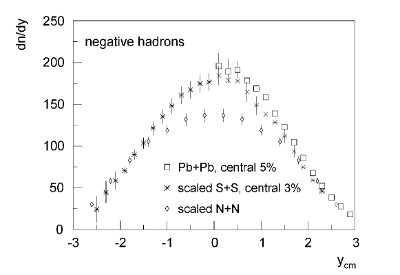
Figure 9.7: $\eta$ distribution of negative hadrons at SPS (shown as $y_{\pi}$ in the center-of-mass). Data are from Ref. [105].

The collision systems and beam energies are from central $\mathrm{Pb}+\mathrm{Pb}$ @ $p_{\mathrm{beam}}=158$ A$\mathrm{GeV/}c$ (hollow squares), central S+S @ $p_{\mathrm{beam}}=200$ A$\mathrm{GeV/}c$ (asterisks), and minimum bias nucleon-nucleon collisions are also shown (hollow rhombi). The data are shown as $dN/dy$ vs. $y$ where $y$ is calculated assuming the pion mass. The shape of the distribution is peaked around mid-rapidity in contrast to the relatively flat region we find at $\sqrt{s_{{}_{\mathrm{NN}}}}$ = 130 $\mathrm{GeV}$. The forward and backward region should show deviations from this behaviour, and it is interesting to study the size of the flat mid-rapidity region. The forward TPC’s in STAR will be in a position to answer this question. From other experiments, results from the PHOBOS collaboration [160] suggest that the plateau region extends up $|\eta|\lesssim 1.5$. The ratio of positive to negative particles $\mbox{$h^{+}$}/\mbox{$h^{-}$}\ =1.025\pm 0.004$ already indicate that the mid-rapidity region is not net-baryon free, as has also been reported by STAR [161] and BRAHMS [162] for the $\mbox{$\bar{p}$}/p$ ratio.

Lower Limit on Energy Density

With the $h^{-}$ multiplicity and $\langle p_{\perp}\rangle$ we can return to the question of estimating the energy density. As discussed in Section 2.2.1, we can only obtain a lower limit with these simple observables. We already stated that there is no reliable guidance as to the value of the initial formation time of the system, $\tau$ in Eq. 2.14. We assume a value of 1$\mbox{$\mathrm{fm}$}/c$, similar to the one adopted at SPS energies, although the system might equilibrate faster at RHIC energies. This is not the only assumption that goes into such an estimate. The initial energy density is also modified, possibly by a large amount, by the longitudinal expansion. Transversal expansion does not change $d\mbox{$E_{\perp}$}/dy$, but is not known how much longitudinal work is done by the system during the expansion. In this sense, it could be misleading to use the initial formation time $\tau$ but a final $d\mbox{$E_{\perp}$}/dy$. Since we measure multiplicity instead of transverse energy, this might turn out to be a better estimate since $dN/dy$ is approximately conserved during the expansion. However, it is more difficult to estimate the time dependence of $\langle p_{\perp}\rangle$. The temperature of the system decreases with time, but the collective flow increases. In the best case, both effects would cancel, but it is more likely that the build up of flow does not fully compensate the decrease in temperature. This also results in an estimate of the energy density that is a lower limit with respect to $\langle p_{\perp}\rangle$. It is also a pre-requisite that the behaviour of the system in the initial stages can be modelled via hydrodynamics. Given a set of energy-momentum conservation and particle number conservation equations along with an equation of state, one can then calculate the energy density, pressure and entropy density of the system. If the entropy density is approximately conserved during the expansion, and under the assumption that the entropy density is approximately proportional to the particle multiplicity in the final state [108, 59], then one can estimate the energy density as in Eq. 2.14.

The estimate under these assumptions proceeds as follows. For central collisions, we have $dN_{ch}/d\eta=567$ and $\langle p_{\perp}\rangle$= 0.511 $\mathrm{GeV/}c$. We could also use $\langle\mbox{$m_{\perp}$}\rangle$ instead of $\langle p_{\perp}\rangle$because one should not neglect the masses. In the best of all worlds one actually would obtain the $\langle\mbox{$m_{\perp}$}\rangle$ for each particle and do a sum weighing by the fraction each particle contributes to the total $h^{-}$ distribution. Since we already mentioned the larger uncertainties that go into the estimate, such refinements can be ignored. In addition we do not know $\langle p_{\perp}\rangle$ for kaons and protons yet, nor do we know the ratios $K^{-}$/$h^{-}$, and $\bar{p}$/$h^{-}$to a degree that we can do considerably better than the simple assumption. Since we measure only the energy density carried by the charged hadrons, we also use Bjorken’s guess $\epsilon\simeq\epsilon_{ch}\times 1.5$. The resulting equation is:

$$\epsilon\geq 1.5\times\ \langle\mbox{$m_{\perp}$}\rangle\frac{dN_{ch}}{dy}\frac{1}{\pi r_{0}^{2}A^{2/3}\tau}$$ (9.2)

The parameters we enter into the formula are the following. We use the same value of $\tau=1$ fm to compare to SPS (although it probably takes less time to equilibrate the system at RHIC energies). This also allows the estimate to be scaled to a different formation time once it is better determined.

The radius ($r=r_{0}\times A^{1/3}$) we use can be simply taken as the one for $b=0$. We must then extrapolate the multiplicity, since it was measured for finite impact parameter. In the geometrical model, 5% corresponds to roughly $b=0-3$ fm. For head-on collisions $b=0$ the $h^{-}$ multiplicity increases with respect to the 5% most central by roughly 14% ($\mbox{$N_{h^{-}}$}\sim 320$ for $b=0$ from Fig. 9.1). In addition, we are measuring $dN/d\eta$ not $dN/dy$. We can use the estimate of $dN/dy$ from the fit to the $\eta$ distributions using the Jacobian $dy/d\eta$.

We then have the parameters $\tau=1$ fm, $A=197$, $dN_{ch}/dy=(295+304)\times 1.14=682$, $\langle\mbox{$m_{\perp}$}\rangle=\sqrt{\mbox{$\langle p_{\perp}\rangle$}^{2}+\langle m\rangle^{2}}=\sqrt{0.511^{2}+0.171^{2}}=0.538$ which we can insert into Eq. 9.2 obtaining

$$\epsilon\gtrsim\frac{1.5\times 682\times 0.538}{\pi\times 1.16^{2}\times 197^{2/3}}=3.9\pm 0.4\mbox{$\mathrm{GeV}$}/\mbox{$\mathrm{fm}$}^{3}$$ (9.3)

The $\sim 10\%$ systematic uncertainty is based on variations of $\langle p_{\perp}\rangle$ and the $h^{-}$, $h^{+}$ multiplicity estimates within their systematic uncertainties.

This is actually somewhat small when one consider that NA49 reports 3.2 $\mbox{$\mathrm{GeV}$}/\mbox{$\mathrm{fm}$}^{3}$ for Pb+Pb via calorimetry (d$E_{\perp}$/d$\eta$). Using tracking they get however 2.6 $\mbox{$\mathrm{GeV}$}/\mbox{$\mathrm{fm}$}^{3}$ [163] for charged particles. The rather small difference between 3.9 and the NA49 result 3.2 also points to the fact that $\tau$ should indeed be smaller for RHIC energies. Other scenarios, such as a denser core and a less denser shell, cannot be probed with this simple method since this is just the average density of the source volume. It is probably best to obtain estimates from actual hydrodynamical simulations that reproduce measured data (e.g. particle yields and spectra, elliptic and radial flow) and obtain from these calculation ranges of values for the relevant parameters, i.e. excluded regions of $\epsilon$. However, for a mid-rapidity region with almost zero baryochemical potential, Figure 2.2 already indicates that at $T=1.5\ \mbox{$T_{c}$}$, the energy density in the deconfined phase (for the case of 2+1 flavour QCD) is $\epsilon\approx 3.5\ \mbox{$\mathrm{GeV}$}/\mbox{$\mathrm{fm}$}^{3}$, so our simple estimate would indicate a favorable environment to reach the deconfined phase.

9.4 Centrality dependence

9.4.1 Centrality selection

It is interesting to study how the distributions are affected by the centrality of the collision. As we mentioned in the discussion of the Glauber model, it is not possible to experimentally determine the impact parameter of the collision. In practice, any study on centrality dependence relies on selecting ensembles of events based on an observable correlated with the impact parameter. Typically these can be transverse energy production, or the charged particle multiplicity of the event. That is why the study of charged hadrons is of primary concern in further studies of heavy ion collisions, such as strangeness production. The focus of the current work however, is the study of charged hadrons, so to study the centrality dependence of charged hadron production is somewhat ill-defined. The approach we followed for the centrality dependence relies on a selection of events based on the ZDC and CTB trigger signals, Figure 8.1. The most central collisions are studied by selecting events below a ZDC threshold, Figure 9.8(a).

 

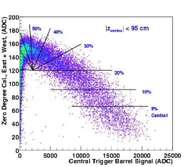
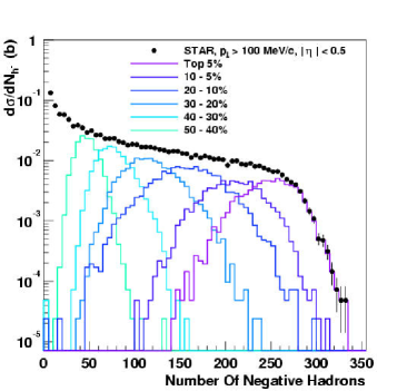
Figure 9.8: Centrality classes for $h^{-}$ analysis. Left panel: cuts in ZDC vs. CTB. Right panel: Resulting classes in the $h^{-}$ multiplicity distribution.

This leads to an ambiguity, since both central and peripheral collisions can have a low ZDC signal, so we set a CTB cut only to break this ambiguity (the cut was set at 8500 ADC counts, not shown in the figure in the interest of clarity). This approach works up to a point, since the ZDC signal turns around and becomes correlated with multiplicity instead of anti-correlated, and we must therefore abandon the the simple ZDC threshold cuts in place of cuts in both ZDC and CTB. Figure 9.8, left panel, shows the cuts in ZDC vs. CTB signals; the right panel shows the resulting event selection in the $h^{-}$ multiplicity distribution for reference.

9.4.2 $p_{\perp}$ and $\eta$ vs. Centrality

With the previous centrality selections, we obtain a $d^{2}N/d\mbox{$p_{\perp}$}d\eta$ distribution for each event sample. We again apply the tracking corrections (Sec. 8.2) for each event and accumulate the corrected distributions for each centrality class. The $\eta$ distribution for the different centrality bins is shown in Fig. 9.9.

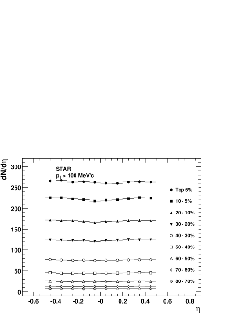
Figure 9.9: The $h^{-}$ $\eta$ distribution for different centralities.

The shape of the distributions at mid-rapidity ($|\eta|<0.5$) is very similar for all the centrality selections.

$\sigma\ (\%)$	$\langle p_{\perp}\rangle$ [$\mathrm{GeV/}c$]	$dN/d\eta$ (Meas.)	$dN/d\eta$ (Extrap.)	$\langle\mbox{$N_{\mathrm{part}}$}\rangle$	$\langle\mbox{$N_{\mathrm{coll}}$}\rangle$	$\langle b\rangle$ $\mathrm{fm}$
0 - 5%	0.511	266.5	289.8	$345\pm 7$	$1050\pm 19$	$2.3\pm 0.2$
5-10%	0.511	222.5	242.2	$289\pm 9$	$826\pm 25$	$4.3\pm 0.3$
10-20%	0.509	169.7	184.9	$221\pm 4$	$566\pm 10$	$5.8\pm 0.3$
20-30%	0.506	123.5	134.7	$152\pm 9$	$336\pm 25$	$7.5\pm 0.3$
30-40%	0.495	76.1	83.1	$102\pm 4$	$209\pm 15$	$8.7\pm 0.3$
40-50%	0.482	44.7	48.9	$63\pm 4$	$105\pm 4$	$10.1\pm 0.4$
50-60%	0.467	24.4	26.8	$35\pm 3$	$36\pm 5$	$11.2\pm 0.6$
60-70%	0.453	12.7	13.9	$20\pm 2$	$22\pm 4$	$12.0\pm 0.7$
70-80%	0.448	7.1	7.8	$9\pm 4$	$9\pm 4$	$12.6\pm 1.1$

Table 9.1: $\langle p_{\perp}\rangle$ and $dN_{h^{-}}/d\eta$ (in the region $|\eta|<0.5$) for various centralities selected as fractions of the cross section $\sigma_{\mathrm{AuAu}}$ (Fig. 9.8). The quantities statistically related to the multiplicity using a Glauber model calculation are also shown for reference.

The $p_{\perp}$ distribution for the different centrality classes is shown in Fig. 9.10. The $dN/d\eta$ and $\langle p_{\perp}\rangle$ values are collected in Table 9.1 while the $p_{\perp}$ distributions for the various centralities are collected in Table 9.2.

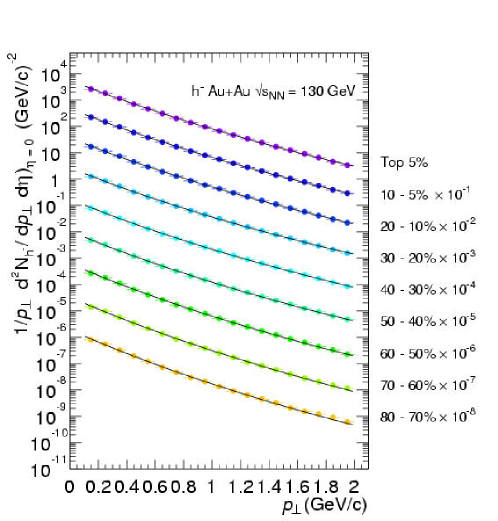
Figure 9.10: The $h^{-}$ $p_{\perp}$ distribution for different centralities. The data are scaled down by successive powers of 10 for display purpose.

$p_{\perp}$	Fraction of $\sigma_{\mathrm{hadronic}}$
($\mathrm{GeV/}c$)	0-5%	5-10%	10-20%	20-30%	30-40%
0.15	2226.0 $\pm$ 94.8	2195.9 $\pm$ 84.0	1689.4 $\pm$ 53.6	1244.6 $\pm$ 42.5	787.3 $\pm$ 21.6
0.25	1729.1 $\pm$ 36.9	1514.3 $\pm$ 52.5	1162.0 $\pm$ 33.3	855.7 $\pm$ 26.4	537.8 $\pm$ 13.3
0.35	1117.1 $\pm$ 26.1	965.8 $\pm$ 34.5	734.8 $\pm$ 21.8	532.6 $\pm$ 17.0	331.2 $\pm$ 8.6
0.45	732.2 $\pm$ 13.7	588.7 $\pm$ 22.6	450.1 $\pm$ 14.3	326.3 $\pm$ 11.2	201.4 $\pm$ 5.6
0.55	478.8 $\pm$ 7.3	381.8 $\pm$ 15.9	291.2 $\pm$ 10.1	211.2 $\pm$ 7.9	130.1 $\pm$ 4.0
0.65	304.3 $\pm$ 6.0	251.2 $\pm$ 11.5	190.0 $\pm$ 7.2	137.4 $\pm$ 5.7	83.8 $\pm$ 2.8
0.75	204.7 $\pm$ 4.0	169.6 $\pm$ 8.5	128.6 $\pm$ 5.3	92.7 $\pm$ 4.2	56.4 $\pm$ 2.1
0.85	139.5 $\pm$ 4.6	115.0 $\pm$ 6.3	86.9 $\pm$ 4.0	63.6 $\pm$ 3.1	38.0 $\pm$ 1.5
0.95	97.6 $\pm$ 2.0	80.7 $\pm$ 4.8	60.4 $\pm$ 3.0	43.8 $\pm$ 2.4	26.5 $\pm$ 1.2
1.05	68.4 $\pm$ 1.9	56.3 $\pm$ 3.7	43.1 $\pm$ 2.3	31.2 $\pm$ 1.8	18.47 $\pm$ 0.89
1.15	47.0 $\pm$ 1.5	39.8 $\pm$ 2.8	30.3 $\pm$ 1.8	21.7 $\pm$ 1.4	12.71 $\pm$ 0.67
1.25	34.2 $\pm$ 1.2	28.0 $\pm$ 2.2	21.4 $\pm$ 1.4	15.33 $\pm$ 1.07	9.03 $\pm$ 0.51
1.35	23.8 $\pm$ 1.0	20.1 $\pm$ 1.7	15.24 $\pm$ 1.06	10.95 $\pm$ 0.83	6.33 $\pm$ 0.39
1.45	16.6 $\pm$ 0.9	14.20 $\pm$ 1.29	10.99 $\pm$ 0.82	7.69 $\pm$ 0.63	4.50 $\pm$ 0.30
1.55	11.72 $\pm$ 0.74	10.46 $\pm$ 1.02	7.91 $\pm$ 0.64	5.70 $\pm$ 0.50	3.25 $\pm$ 0.23
1.65	8.69 $\pm$ 0.46	7.63 $\pm$ 0.79	5.76 $\pm$ 0.50	4.02 $\pm$ 0.38	2.32 $\pm$ 0.18
1.75	6.20 $\pm$ 0.43	5.61 $\pm$ 0.62	4.18 $\pm$ 0.39	2.96 $\pm$ 0.30	1.68 $\pm$ 0.14
1.85	4.44 $\pm$ 0.39	3.93 $\pm$ 0.47	2.99 $\pm$ 0.30	2.14 $\pm$ 0.24	1.20 $\pm$ 0.11
1.95	3.38 $\pm$ 0.32	2.88 $\pm$ 0.37	2.20 $\pm$ 0.23	1.57 $\pm$ 0.18	0.851 $\pm$ 0.081
$p_{\perp}$	Fraction of $\sigma_{\mathrm{hadronic}}$
($\mathrm{GeV/}c$)	40-50%	50-60%	60-70%	70-80%
0.15	472.0 $\pm$ 14.9	268.5 $\pm$ 10.7	143.5 $\pm$ 6.4	80.6 $\pm$ 4.8
0.25	325.3 $\pm$ 9.3	183.1 $\pm$ 6.6	97.1 $\pm$ 3.9	54.7 $\pm$ 2.9
0.35	198.8 $\pm$ 5.9	110.1 $\pm$ 4.1	57.8 $\pm$ 2.4	32.6 $\pm$ 1.8
0.45	119.1 $\pm$ 3.8	65.3 $\pm$ 2.7	34.5 $\pm$ 1.6	19.3 $\pm$ 1.2
0.55	76.0 $\pm$ 2.7	41.2 $\pm$ 1.8	21.2 $\pm$ 1.0	11.91 $\pm$ 0.78
0.65	48.8 $\pm$ 1.9	26.3 $\pm$ 1.3	13.37 $\pm$ 0.72	7.26 $\pm$ 0.53
0.75	32.3 $\pm$ 1.4	16.90 $\pm$ 0.92	8.68 $\pm$ 0.50	4.67 $\pm$ 0.37
0.85	21.5 $\pm$ 1.0	11.42 $\pm$ 0.68	5.56 $\pm$ 0.36	2.97 $\pm$ 0.26
0.95	15.12 $\pm$ 0.76	7.78 $\pm$ 0.51	3.84 $\pm$ 0.26	2.08 $\pm$ 0.20
1.05	10.03 $\pm$ 0.56	5.18 $\pm$ 0.37	2.52 $\pm$ 0.19	1.35 $\pm$ 0.137
1.15	6.89 $\pm$ 0.41	3.50 $\pm$ 0.27	1.73 $\pm$ 0.14	0.910 $\pm$ 0.098
1.25	4.97 $\pm$ 0.32	2.49 $\pm$ 0.21	1.14 $\pm$ 0.10	0.629 $\pm$ 0.072
1.35	3.50 $\pm$ 0.24	1.71 $\pm$ 0.15	0.828 $\pm$ 0.072	0.449 $\pm$ 0.053
1.45	2.47 $\pm$ 0.18	1.23 $\pm$ 0.12	0.592 $\pm$ 0.053	0.317 $\pm$ 0.039
1.55	1.76 $\pm$ 0.14	0.866 $\pm$ 0.087	0.403 $\pm$ 0.037	0.210 $\pm$ 0.027
1.65	1.24 $\pm$ 0.11	0.630 $\pm$ 0.066	0.279 $\pm$ 0.026	0.154 $\pm$ 0.020
1.75	0.940 $\pm$ 0.082	0.438 $\pm$ 0.049	0.205 $\pm$ 0.019	0.120 $\pm$ 0.014
1.85	0.652 $\pm$ 0.061	0.330 $\pm$ 0.038	0.151 $\pm$ 0.013	0.089 $\pm$ 0.010
1.95	0.474 $\pm$ 0.046	0.226 $\pm$ 0.027	0.115 $\pm$ 0.009	0.061 $\pm$ 0.006

Table 9.2: $h^{-}$ yield $d^{2}N/(\mbox{$p_{\perp}$}\ d\mbox{$p_{\perp}$}\ d\eta)$ at $\eta=0$ for different centralities.

It is instructive to do a comparison between peripheral and central $p_{\perp}$ distributions. It is easier to study differences in the distributions by plotting the ratios of the $p_{\perp}$ spectra, since slight changes in curvature are difficult to see in a log scale such as in Fig. 9.10. As a reference, we take the shape of the measured $p_{\perp}$ distribution for the most peripheral bin ($70-80\%$ of $\sigma_{\mathrm{AuAu}}$).

 

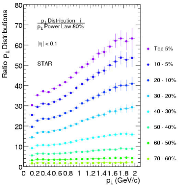
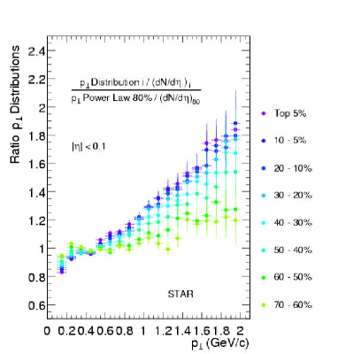
Figure 9.11: Ratio of the $p_{\perp}$ distributions for different centralities to the $p_{\perp}$ spectrum of the most peripheral bin (70-80%). Left panel: simple ratio of the data. Right panel: Ratio of data points to the power law fit to the most peripheral bin including a normalization of each distribution to the corresponding mid-rapidity density $dN/d\eta$ of each sample.

We then take the ratio of each of the distributions in Fig. 9.10 to the most peripheral. The simplest exercise is to take the ratio without any further scaling. This is shown in Fig. 9.11(a). If we take the most peripheral distribution as the one which most closely should follow the spectrum from $pp$ or $p\bar{p}$ collisions, we see how the shape of the $p_{\perp}$ distributions change with centrality. Similarly to the $p\bar{p}$ comparison, we see an increase in the $h^{-}$ yield with increasing $p_{\perp}$ for a particular centrality selection compared to the peripheral distribution. We also see that the excess at fixed $p_{\perp}$increases with centrality. This is more easily seen in a double ratio, where we normalize each $p_{\perp}$ distribution by the corresponding $dN/d\eta$, i.e. by the integral with respect to $p_{\perp}$. This double-ratio is shown in Fig. 9.11. The double-ratio curves then meet at low-$p_{\perp}$ independent of centrality, and the rise with increasing $p_{\perp}$ is evident. We find that for the most central collisions, the $h^{-}$ yield at 2 $\mathrm{GeV/}c$ is almost a factor of 2 larger than expected from a superposition of peripheral collisions that would integrate to the same yield. This change in behaviour is consistent with the presence of collective effects such as increased radial flow for central collisions. However, as mentioned before, the $p_{\perp}$ spectrum for even the most central collisions still does not reach the expected scaling with $N_{\mathrm{coll}}$ at 2 $\mathrm{GeV/}c$. The measurement of the $p_{\perp}$ distributions at higher $p_{\perp}$ will help be an interesting extension to these studies, as they will shed more light on the modification of the $p_{\perp}$ spectra, e.g. whether the “Cronin” effect observed in $pA$ collisions and lower energy $AA$ collisions should be seen at these moderate momenta, and if so, whether the jet quenching hypothesis is able to reproduce the centrality dependence of the $p_{\perp}$ ratios such as Fig. 9.5 and Fig. 9.11.

Figure 9.12 shows the

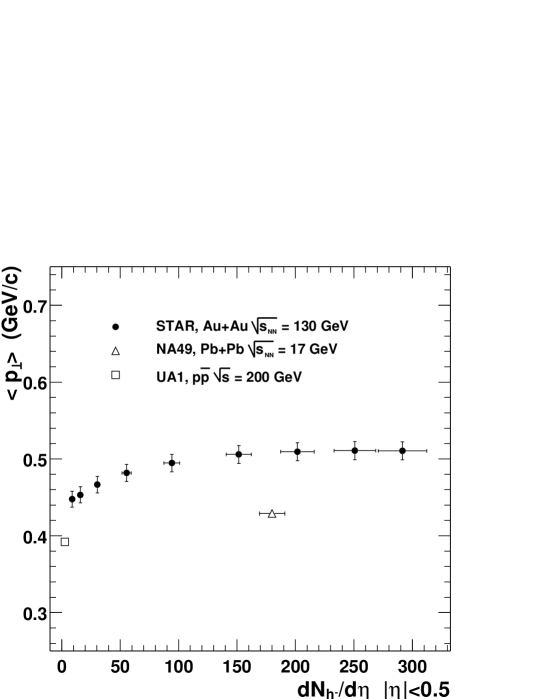
Figure 9.12: The multiplicity dependence of $\langle p_{\perp}\rangle$ for $h^{-}$. The values obtained from the UA1[96] and NA49[105] $p_{\perp}$ distributions in Fig. 9.5 are also shown.

multiplicity dependence of $\langle p_{\perp}\rangle$ for $h^{-}$. We use the fitted parameters to the power law in Fig. 9.10 to obtain $\langle p_{\perp}\rangle$, the corresponding multiplicity is obtained by averaging the measured yield in the region $|\eta|<0.5$, $0.1<\mbox{$p_{\perp}$}<2\mbox{$\mathrm{GeV/}c$}$ (Fig. 9.9) and extrapolating to all $p_{\perp}$ using the power law. This has the effect that the average multiplicity measured in the wider slice is higher (267, compared to 261). The data are collected in

Table  9.1, which shows the multiplicity and $\langle p_{\perp}\rangle$ obtained from the spectra for the different fractions of cross section. The error bars representing the systematic uncertainty are 2% for $\langle p_{\perp}\rangle$, 6.4% for measured and 7.1% for extrapolated $dN/d\eta$. By using the power-law fits to the $p_{\perp}$ distributions in this range, we obtain the missing fraction in order to obtain a total yield ($\sim 7\%$ for $0<\mbox{$p_{\perp}$}<0.1$ and $1\%$ for $\mbox{$p_{\perp}$}>2\ \mbox{$\mathrm{GeV/}c$}$). The centrality selection is based on cuts in ZDC and CTB trigger signals as shown in Fig.9.8.

We see an increase in $\langle p_{\perp}\rangle$ in the first peripheral bins and then a saturation. The value of $\langle p_{\perp}\rangle$ increases by 18% compared to SPS energies, when comparing to central collisions. To put into perspective the stiffness of the observed $\mathrm{Au}+\mathrm{Au}$ $p_{\perp}$ spectra, the measured $\langle p_{\perp}\rangle$ at $\sqrt{s}$ = 900 $\mathrm{GeV}$ reported in [96] is $\langle p_{\perp}\rangle$ = $0.447\pm 0.003$ $\mathrm{GeV/}c$. At the highest Tevatron energies, CDF reports [164] $\langle p_{\perp}\rangle$ = $0.495\pm 0.014$. The saturation of $\langle p_{\perp}\rangle$ contrasts the structure proposed in Ref. [65], where the qualitative dependence for a first order transition (under the assumption that the central multiplicity is approximately proportional to the $sV$, where $V$ is the volume of the system and $s=\epsilon+p$ is the entropy density in Landau hydrodynamics, and that $\langle p_{\perp}\rangle$ reflects the temperature of the system) should be an initial correlation between $dN/d\eta$ and $\langle p_{\perp}\rangle$, followed by a saturation, and then a subsequent rise. We find no such structure. This behaviour helps to strengthen the growing evidence against a strong first order transition. In addition, it is also consistent with current expectations of a second order phase transition region at higher baryo-chemical potentials with a critical point followed by a region of a smooth cross over between the QGP and hadron gas phase below some as yet undetermined value for $\mu_{B}$. Initial estimates from particle ratios at RHIC yield values of $\mu_{B}\simeq\ 45\ \mbox{$\mathrm{MeV}$}$, which would then most probably place RHIC collisions at this energy in the cross-over region. This will of course need to be studied with more sophisticated analyses, in particular, an interesting future direction could be the measurement of the $\langle p_{\perp}\rangle$ vs. $dN/d\eta$, along with $\langle p_{\perp}\rangle$ fluctuations event-by-event, studied for different centre-of-mass energies or collision systems to search for the possible critical point. Theoretical guidance in this direction would also be fruitful in this search.

Chapter 10 Results and Discussion: Identified Pions

The next step in the analysis of charged particles is to use the particle identification capabilities of the TPC. This allows us to select a specific particle for further study. The first natural candidate is the $\pi$ meson, the lightest of the hadrons and the most copiously produced particle in a high energy heavy ion collision.

10.1 Raw Yields

The starting point to obtain the raw yields for the identified particle analyses is Fig. 6.2. One can obtain the raw yields of pions, kaons and protons (and their antiparticles) selecting events according to their centrality and fitting the $\frac{dE}{dx}$ distribution in a given y-$p_{\perp}$ phase space cell. The procedure adopted here is a variation from this which offers a few advantages. Tracks were selected according to quality criteria based on number of points on the track and on the pointing accuracy to the primary event vertex. The cuts used in the pion analysis were more stringent than the ones used for the $h^{-}$ analysis. This was done mainly to select tracks with a good $\frac{dE}{dx}$ resolution as it depends mainly on the number of valid ionization samples, see Fig.6.3.

For this analysis, we followed a procedure similar to the one outlined in Ref. [165] for ionization measurements. We use the truncated mean to estimate the ionization of a given track ($I_{m}$). The expected ionization for a given momentum and a given mass hypothesis ($I_{h}$)is known to an accuracy of better than 0.1%, as represented by the curves in Fig.6.2. We then construct the $z$ variable defined as

$$z=\ln\left(\frac{I_{m}}{I_{h}}\right)$$ (10.1)

The $z$ variable follows a Gaussian distribution with mean zero for a given particle population and with standard deviation given by the measured $\frac{dE}{dx}$ resolution as a function of the number of $\frac{dE}{dx}$ samples, Fig.6.3. The mean will be zero independent of momentum for the given particle species under consideration, since the momentum dependence is contained in $I_{h}$. By incorporating $I_{h}$ and the measured resolution $\sigma_{dE/dx}$, we can obtain a new distribution, $Z_{\pi}$, that has unit width and zero mean for the particle of interest: $Z_{\pi}=z_{\pi}/\sigma_{dE/dx}$.

Fig. 10.1 shows the result of fitting to the $Z$ distributions in different phase-space bins. Shown is the region 0.2 < y < 0.3 for 6 different $p_{\perp}$ bins in steps of 50 $\mathrm{MeV/}c$ starting from $p_{\perp}$= 0.3 $\mathrm{GeV/}c$.

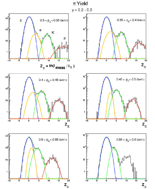
Figure 10.1: Fits to the $Z_{\pi}$ distribution to extract the yield of $\pi^{-}$. Shown is the region $0.2<y<0.3$ and $0.3<\mbox{$p_{\perp}$}<0.6\ \mbox{$\mathrm{GeV/}c$}$.

The abscissa is in log scale, and the ordinate is in linear scale (note that $Z_{\pi}$ is already the log of the ionization). Strictly, only the pion population should follow a Gaussian in the $z_{\pi}$ variable. One can of course construct a $z$ variable for the other species ($z_{K}$, $z_{p}$ and $z_{e}$) in order to extract their yields. The analysis of the other particle species is being carried out in STAR also. Here we focus on the pions which are the bulk of the produced particles as can be seen from the relative heights of the different Gaussians in the plot. The figure shows the result of the different fits using a Gaussian for each of the particle species. The pion yield is extracted from the Gaussian centered at zero. In the lower right panel, the electron yield is small enough and close enough to the kaon population that one can use a single Gaussian function. The fit also stops at $Z_{\pi}=5$ in the bottom right panel, thus the anti-proton Gaussian is not shown.

10.2 Corrections

The corrections applied to the raw data follow the same procedure as for the $h^{-}$ distribution with a few important differences. First of all, we chose to do them in cells of ($y,\mbox{$p_{\perp}$}$) instead of ($\eta,\mbox{$p_{\perp}$}$). The acceptance and efficiency use the embedding procedure as in the $h^{-}$ analysis. Embedding was done in the region .1 < $p_{\perp}$ < 2 $\mathrm{GeV/}c$, and |$y$|<1. For the lowest $p_{\perp}$ bin, 50 < $p_{\perp}$ < 100 $\mathrm{MeV/}c$, we used a full hijing simulation. The efficiency obtained from embedding is shown in Fig.10.2.

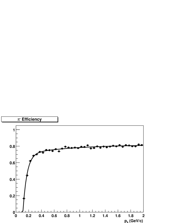
Figure 10.2: The track reconstruction efficiency as a function of $p_{\perp}$  for $\pi^{-}$ mesons. The efficiency is lower than in Fig. 8.7 as the requirements for tracks in the $\frac{dE}{dx}$ analysis are more stringent than for the $h^{-}$ analysis.

The stringent requirement on 24 or more fit points on the track effectively removed the need to undertake a split track correction. For the momentum range $\mbox{$p_{\perp}$}<0.6\ \mbox{$\mathrm{GeV/}c$}$ the distortion of the spectrum due to resolution effects was found to be negligible. This fact and the good statistics of the sample allowed for a much finer bin size in the $p_{\perp}$ spectrum. This was also desirable since this narrowed the phase space where the fits were made to obtain the yield. Event though the use of the $z$ variable fixes the region where the pions are found, the other particles will still vary with momentum. Therefore, a narrower $p_{\perp}$ bin will reduce this effect making the fits more stable. The final spectrum was also corrected for the products of weak decays and for the expected contribution of pions resulting from secondary interactions. Since for this analysis the requirement on the distance of closest approach to the primary interaction vertex was set at 1 cm, the background correction was smaller than for the $h^{-}$ analysis, and was found to be $\lesssim 5\%$. We present now the resulting distributions for identified $\pi^{-}$ mesons.

10.3 $p_{\perp}$ and $m_{\perp}$ Distributions

10.3.1 Results

We first look at the spectra for central events. Figure 10.3 shows the $p_{\perp}$ distribution for $\pi^{-}$ for the 5% most central collisions (selected by a cut on raw $h^{-}$ multiplicity). The data are grouped for different bins in rapidity, and scaled by successive powers of 2 for the figure.

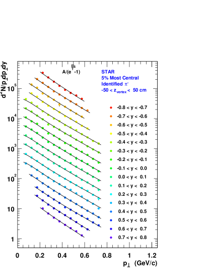
Figure 10.3: $\pi^{-}$ $p_{\perp}$ distribution for central collisions. The different bins in rapidity are scaled by successive powers of 2 for display purpose.

The more common way to show such a distribution is in transverse mass, $m_{\perp}$, and this is shown in Figure  10.4.

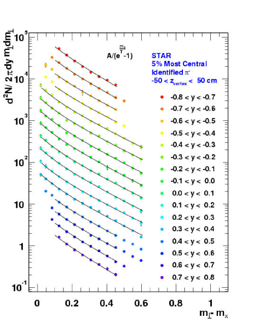
Figure 10.4: $\pi^{-}$ $d^{2}N/(2\pi\ dy\ \mbox{$m_{\perp}$}d\mbox{$m_{\perp}$})$ distribution for central collisions. The rapidity bins are scaled by successive powers of 2 for display purpose.

The main corrections applied to the raw data are acceptance, efficiency and contributions from weak decay background and secondary interactions. The effect of energy loss in the determination of the $\pi^{-}$ momenta was found to be less than 2% at 100 $\mathrm{MeV/}c$, decreasing rapidly for larger momenta. We also studied the effect of momentum resolution as for the $h^{-}$ data and found that the main effect was the feeding of the lowest $p_{\perp}$ bin from its nearest neighbour. The change in the slope for $\mbox{$p_{\perp}$}\ >100\ \mbox{$\mathrm{MeV/}c$}$ was found to be $\ll 1\%$. The data for the central rapidity bins, $|y|<0.4$, was obtained in the range $0.05<\mbox{$p_{\perp}$}<0.75\ \mbox{$\mathrm{GeV/}c$}$, which accounts for $\sim 85\%$ of the total yield. As we go towards the forward and backward regions, the $p_{\perp}$ range where the identification via $\frac{dE}{dx}$ in the TPC can be done shrinks, and we can only measure in the range 0.2 < $p_{\perp}$ < 0.6 $\mathrm{GeV/}c$.

10.3.2 Discussion

Pions are the bulk of the produced particles, they are the lightest of the hadrons and have large interaction cross sections in nuclear matter; they are therefore expected to thermalize easily. In addition, their spectra are the least affected by a given collective transverse flow velocity, and are thus good probes to study the kinetic freeze-out properties of the system. The pion data are fit with a Bose-Einstein distribution of the form $A/(\exp(\mbox{$m_{\perp}$}/T)-1)$. Typically, these distributions are fit with a Boltzmann distribution [120]. The data at low-$p_{\perp}$ fit with a Boltzmann distribution always seemed to show an enhancement. This partly was attributed to contributions coming from resonance decays. There are also enhancements in the high-$p_{\perp}$ region which can arise from contributions of pions coming from high momentum transfer of partons early in the collision. A consequence of all these structures was that simple Boltzmann fits to the same spectrum would lead to different slope parameters depending upon the $p_{\perp}$ region included in the fit. Since we focus here on the low $p_{\perp}$ part of the spectrum, and since pions are bosons, we chose to fit the data with a Bose-Einstein distribution. We find that this naturally gives an enhancement in the very low $p_{\perp}$ region of the spectrum. Also, we have already estimated the contribution from weak decays to the distribution and corrected for this effect. We have not estimated the contribution from resonance decays however. We fit the data over the measured range, instead of excluding the low momentum data from the fit, and find no significant enhancement at low $p_{\perp}$. The absence of a noticeable contribution from resonances might be due to reinteraction of the daughter decay particles. A fit using a Boltzmann distribution for the range above $\mbox{$p_{\perp}$}=0.3\ \mbox{$\mathrm{GeV/}c$}$ causes a variation in the slope parameters of $\sim 10\ \mbox{$\mathrm{MeV}$}$. Since the data at forward and backward rapidity have a smaller range in $p_{\perp}$  as a systematic check we performed a fit restricted to the $p_{\perp}$ range which was measured for all the rapidity bins. This resulted in a change in the slope parameters of 5-10 $\mathrm{MeV}$ for the $|y|<0.4$ spectra. We find the slope parameter for the central collisions to be $\mbox{$T_{\mathrm{eff}}$}=210\ \pm 20\ \mbox{$\mathrm{MeV}$}$, where the systematic uncertainty comes from studying the variation in the slope parameter with several changes, including variations in the fit range, choice of fit function, centrality selection, and analyzing the pions in $\eta$ instead of $y$. The error on $T_{\mathrm{eff}}$ from any particular fit is on the order of $5\ \mbox{$\mathrm{MeV}$}$. The rapidity dependence of the $\pi^{-}$ yield and of the slope parameters is discussed in the following section.

The shape of the low $p_{\perp}$ pion spectra, in contrast to the $h^{-}$ distribution, shows very little change when going from SPS energies to RHIC. The slope parameters reported by NA49 [117] for $\pi^{-}$ near midrapidity are $\mbox{$T_{\mathrm{eff}}$}=188\pm 6\ \mbox{$\mathrm{MeV}$}$ for $\pi^{+}$ and $\mbox{$T_{\mathrm{eff}}$}=192\pm 3\ \mbox{$\mathrm{MeV}$}$ using an exponential fit. WA98 data for $\pi^{0}$ spectra for central collisions yields also similar values of $\mbox{$T_{\mathrm{eff}}$}\simeq 204$ (although fitting the data with a Bessel function, $\mbox{$m_{\perp}$}K_{1}(\mbox{$m_{\perp}$}/\mbox{$T_{\mathrm{eff}}$})$ yields a smaller value of $\mbox{$T_{\mathrm{eff}}$}=155$, so one must be careful when comparing). The pion spectra from NA45 [104] were analyzed in terms of a local inverse slope changing with $m_{\perp}$ to take into account the difference at low and high $p_{\perp}$. For the low $m_{\perp}$ range ($\mbox{$m_{\perp}$}-m_{\pi}<0.8\ \mbox{$\mathrm{GeV/}c^{2}$}$) the local inverse slope is found to be in the range $180-200\ \mbox{$\mathrm{MeV}$}$. The slopes at the AGS have smaller values, E895 finds [115] $\mbox{$T_{\mathrm{eff}}$}\simeq 110\ \mbox{$\mathrm{MeV}$}$. While the initial temperature reached at RHIC is expected to be larger than at the SPS and the AGS, the $\pi^{-}$ spectrum probes the final state. The saturation of the $\pi^{-}$ slope parameter would indicate that the freeze-out temperature, assuming that thermal equilibrium is reached, is the same at SPS and RHIC. This does not mean that the final state is the same, for there is evidence of an increased collective radial flow velocity at RHIC based on the preliminary $p_{\perp}$ distributions of heavier particles from STAR [45, 166]. Since the collective velocity affects the heavier particles the most, the pion inverse slope is the one numerically closer to the actual freeze-out temperature, $T_{\mathrm{f.o.}}$. The slopes of the $K^{-}$ and $\bar{p}$ will be much larger than for the $\pi^{-}$ even if they all freeze out at the same temperature in the presence of large radial flow.

In order to gain further insight into the dynamics of the system, a study of the heavier particle spectra can be made to address the question of radial flow. In a different approach, the combination of the 2-particle correlation results[167] along with the pion spectra is also useful: they determine the 6-dimensional pion phase space density, i.e. the dimensionless average number of pions per 6-dimensional phase space cell $\hbar^{3}$ (see e.g. [168]). Such analyses can help to disentangle the intrinsic freeze-out temperature and the transverse flow velocity. For example, for the 5% most central data, preliminary analysis of the phase space density yield values of $\mbox{$T_{\mathrm{f.o.}}$}\sim 120\ \mbox{$\mathrm{MeV}$}$ and $\langle\beta_{\perp}\rangle\sim 0.53$. This is a rather large flow velocity, yet since the pions are so light, the slope parameter $T_{\mathrm{eff}}$ is only increased to $\sim 200$ $\mathrm{MeV}$, while the slope parameter for the heavier $K^{-}$ increases to $\sim 300\ \mbox{$\mathrm{MeV}$}$ and is even larger for the $\bar{p}$ [45]. The systematics of the centrality dependence of the pion phase space density is a currently active area of study in STAR which will certainly help to shed light on the determination of the kinetic freeze-out conditions of the system.

10.4 Rapidity Distribution

10.4.1 Results

By integrating the $p_{\perp}$ spectra in Figure 10.3 for each of the rapidity bins, we are able to obtain the $dN/dy$ vs. $y$ distribution for $\pi^{-}$. The result is shown in Figure 10.5. Several data points are shown. The black circles are obtained by integrating the $p_{\perp}$ spectrum in the limited $p_{\perp}$ region $0.2-0.6\ \mbox{$\mathrm{GeV/}c$}$ where we have data for $|y|<0.8$. This shows that the measured yield in this region is relatively independent of rapidity. The measured yield in this region is, however, only about half of the total yield. To illustrate the behaviour of the yield in the full available $p_{\perp}$ region ($0.05-0.75\ \mbox{$\mathrm{GeV/}c$}$) for a narrower $y$ region, we plot the data shown as the black squares. Finally, the open circles are the extrapolated yield to all $p_{\perp}$ based on the fits to the data using the Bose-Einstein distribution. We find the pion yield to be $\mbox{$dN/dy$}|_{|y|<0.1}=286\pm 10$ for the 5% most central events.

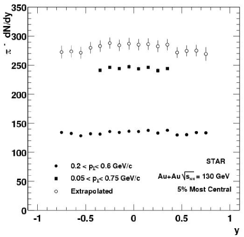
Figure 10.5: $\pi^{-}$ rapidity distribution. The black circles (squares) are obtained summing the yield between $p_{\perp}$ 0.2 - 0.6 $\mathrm{GeV/}c$ (0.05 - 0.75) from Fig. 10.3. The hollow data points are the yields obtained using the fit function extrapolated to all $p_{\perp}$.

Not only is it important to study the yields as a function of rapidity, but it is equally important to examine the rapidity dependence of the slope parameters. At the SPS and at the AGS, they have been found to decrease with increasing $|y|$. The $T_{\mathrm{eff}}$ slope parameter extracted from the Bose-Einstein fit to the data is shown in Figure 10.6.

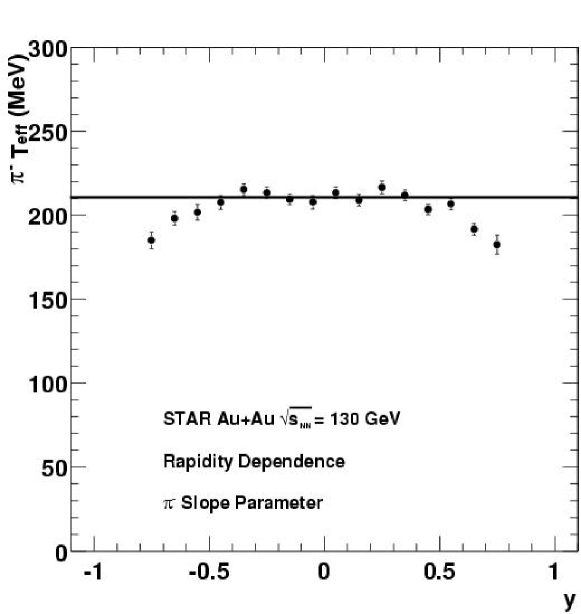
Figure 10.6: $\pi^{-}$ slope parameter for the different rapidity bins from Fig. 10.4. The flat line at $\mbox{$T_{\mathrm{eff}}$}=210$ is the average for $|y|<0.1$

The error bars in the figure are the uncorrelated point-to-point systematic uncertainties on $T_{\mathrm{eff}}$, the overall correlated systematic uncertainty is $\pm 20\ \mbox{$\mathrm{MeV}$}$. The rapidity dependence of the yield, the slope parameter $T_{\mathrm{eff}}$ and $\langle p_{\perp}\rangle$ are collected in

$y$	$dN/dy$	$T_{\mathrm{eff}}$ [$\mathrm{MeV}$]	$\langle p_{\perp}\rangle$ [$\mathrm{MeV/}c$]
-0.75	273 $\pm$ 13	185.0 $\pm$ 5.0	356 $\pm$ 9.9
-0.65	274 $\pm$ 11	198.1 $\pm$ 4.2	376 $\pm$ 8.4
-0.55	273 $\pm$ 10	201.7 $\pm$ 4.6	385 $\pm$ 9.2
-0.45	280 $\pm$ 10	207.5 $\pm$ 4.0	391 $\pm$ 7.9
-0.35	283 $\pm$ 10	215.2 $\pm$ 3.6	397 $\pm$ 7.2
-0.25	288 $\pm$ 10	213.4 $\pm$ 3.1	402 $\pm$ 6.2
-0.15	284 $\pm$ 10	209.5 $\pm$ 3.2	396 $\pm$ 6.4
-0.05	287 $\pm$ 10	207.7 $\pm$ 3.9	394 $\pm$ 7.8
0.05	285 $\pm$ 10	213.3 $\pm$ 3.4	400 $\pm$ 6.8
0.15	286 $\pm$ 10	208.9 $\pm$ 3.4	392 $\pm$ 6.9
0.25	284 $\pm$ 10	216.5 $\pm$ 3.8	404 $\pm$ 7.6
0.35	285 $\pm$ 10	211.9 $\pm$ 3.1	400 $\pm$ 6.2
0.45	272 $\pm$ 10	203.4 $\pm$ 3.2	383 $\pm$ 6.4
0.55	275 $\pm$ 10	206.5 $\pm$ 3.4	388 $\pm$ 6.8
0.65	275 $\pm$ 11	191.5 $\pm$ 4.0	367 $\pm$ 8.0
0.75	269 $\pm$ 14	182.4 $\pm$ 5.6	350 $\pm$ 11.2

Table 10.1: $\pi^{-}$ $dN/dy$, $T_{\mathrm{eff}}$ and $\langle p_{\perp}\rangle$ vs. $y$.

Table 10.1. The $p_{\perp}$ distributions for the most central data for the various $y$ bins are collected in Table 10.3.

10.4.2 Discussion

The rapidity distribution has nearly a plateau shape at mid-rapidity. However, there remains a slight rapidity dependence of the slope parameter $T_{\mathrm{eff}}$. This behaviour is indicative that the idealized boost-invariant mid-rapidity region is not yet reached in $\mathrm{Au}+\mathrm{Au}$ collisions at $\sqrt{s_{{}_{\mathrm{NN}}}}$= 130 $\mathrm{GeV}$. A possible cause for the observed effect can be a change in the baryon content of the system with rapidity. In the presence of radial flow driven by the dominant $\pi^{-}$ mesons, a larger fraction of baryons would take away some of the pion’s kinetic energy, reducing the observed slope parameter. The anti-proton to proton ratios reported by STAR [161] and BRAHMS [162] show a drop in the $\mbox{$\bar{p}$}/p$ ratio from 0.65 at mid-rapidity to 0.41 for the region $y\approx 2$, which already hints at such effects, but a better understanding of the dynamics must wait for the measured baryon yields and the baryon rapidity distributions.

10.5 Centrality Dependence

10.5.1 Centrality Selection

For the $\pi^{-}$ centrality dependence, we chose to do a selection based on the event multiplicity. This is in contrast to the centrality selection for the $h^{-}$ analysis which was based on ZDC and CTB trigger signals. The reason for this choice was simply to use a common set of cuts which would be useful not just for this analysis, but also for other studies such as particle correlations (Hanbury-Brown Twiss) and in particular for the studies of the pion phase space density. Having a standard set of values based on the (uncorrected) $h^{-}$ yield facilitates comparison and combination of different observables. There was a worry that since the pions are the main component of the charged hadron spectra, a centrality selection based on charged multiplicity would introduce a sizable auto-correlation. Certainly, the shape of the $h^{-}$ multiplicity distribution for 5% most central events (the shaded region in Fig. 9.1) would look different by selecting events with a straight cut on uncorrected multiplicity. The mean of this distribution, i.e. the value of $dN/d\eta$ for the region $|\eta|<0.5$, will also shift to higher values by doing such a selection. The question is how significant is this shift. We studied this by selecting the 5% most central events based on uncorrected multiplicity and comparing the mean of the resulting distribution to the mean of the histogram in the shaded region of Figure  9.1. The mean of the histogram using the centrality definition based on multiplicity was 4.5% higher than than the one using the ZDC as centrality definition. The difference in the mean of the histograms using these two centrality definitions will also decrease for more peripheral collisions. We therefore conclude that the differences are not problematic, and when encountered, they can be reconciled by at most a 4.5% effect.

10.5.2 $m_{\perp}$ Distributions vs. Multiplicity

Figure 10.7 shows the $m_{\perp}$ distribution for 10 different centrality selections. The data are taken in the rapidity interval $0<y<0.1$. Again, the data are fit by a Bose-Einstein distribution which agrees well with the spectra even at the lowest $m_{\perp}$. The slope parameters are very similar for the different centralities.

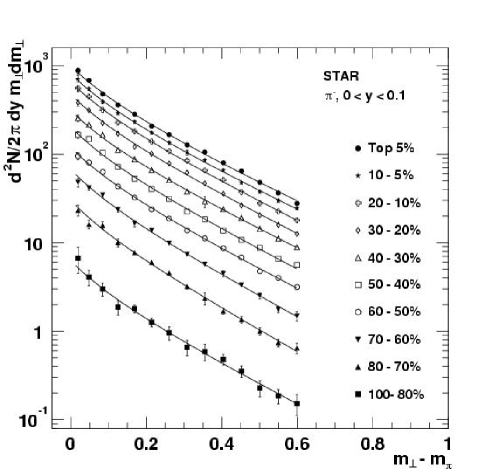
Figure 10.7: $\pi^{-}$ $m_{\perp}$ distribution for different multiplicity selections. The distributions are plotted in the rapidity slice 0 < $y$ < 0.1 units. The data are fit to Bose-Einstein distributions (curves) from which we extract the slope parameter $T_{\mathrm{eff}}$.

They are collected and plotted vs. the $h^{-}$ mean multiplicity of the corresponding centrality bin in Figure 10.8.

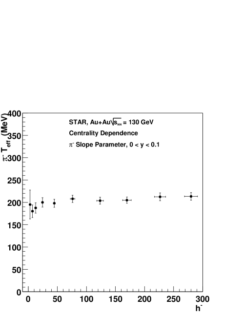
Figure 10.8: Centrality dependence of the slope parameter obtained by a fit to the $\pi^{-}$ $m_{\perp}$ distribution.

The horizontal error bars are the systematic uncertainty in the determination of the mean multiplicity of each centrality bin. The vertical error bars are the uncorrelated systematic uncertainty in the measurement of the slope parameter. For the most peripheral bins, the statistical error is also important, and the error bar is therefore larger.

We see that there is a only a slight dependence of the slope parameter with centrality. The main difference happens for the 2nd and 3d most peripheral bins (the most peripheral bin has a larger error, so it is hard to see a systematic effect). The 2nd most peripheral bin has a slope $\mbox{$T_{\mathrm{eff}}$}=177\pm 8\ \mbox{$\mathrm{MeV}$}$, while the most central bin has a slope $\mbox{$T_{\mathrm{eff}}$}=210\pm 4\ \mbox{$\mathrm{MeV}$}$ (where the errors are the uncorrelated systematic uncertainties for the comparison). This yields an increase of $19\pm 5\%$. The increase occurs rapidly, as the 60% of $\sigma_{\mathrm{AuAu}}$ bin already has a slope parameter of $\mbox{$T_{\mathrm{eff}}$}=196\pm 9\mbox{$\mathrm{MeV}$}$, and from then on the data are consistent with having no further centrality dependence. For comparison, the increase in $h^{-}$ $\langle p_{\perp}\rangle$ from the $70-80\%$ bin to the most central bin is $14\pm 3\%$. In addition, the $h^{-}$ distribution includes a $\bar{p}$ component, and the $\bar{p}$ slope has a stronger centrality dependence than the $\pi^{-}$ slope. At SPS energies, the centrality dependence of the pion slopes was also found to be rather constant. This finding is also in agreement with the argument that the slope of the $\pi^{-}$ spectrum is not changed significantly by the collective expansion.

$\mbox{$m_{\perp}$}-m_{\pi}$ ($\mathrm{GeV/}c^{2}$)	0-5%	5-10%	10-20%	20-30%	30-40%
0.0189	871 $\pm$ 70	707 $\pm$ 57	550 $\pm$ 43	377 $\pm$ 31	254 $\pm$ 21
0.0478	679 $\pm$ 30	544 $\pm$ 25	446 $\pm$ 19	312 $\pm$ 14	214 $\pm$ 9.5
0.0842	473 $\pm$ 25	388 $\pm$ 20	312 $\pm$ 13	224 $\pm$ 9.7	164 $\pm$ 7.0
0.125	357 $\pm$ 12	289 $\pm$ 11	226 $\pm$ 6.9	169 $\pm$ 5.9	111 $\pm$ 3.9
0.169	281 $\pm$ 11	231 $\pm$ 11	180 $\pm$ 6.4	120 $\pm$ 5.2	87.1 $\pm$ 2.8
0.214	206 $\pm$ 7.2	173 $\pm$ 6.7	138 $\pm$ 4.1	100 $\pm$ 2.8	65.7 $\pm$ 2.4
0.261	165 $\pm$ 5.8	134 $\pm$ 5.8	108 $\pm$ 3.2	78.1 $\pm$ 2.1	50.8 $\pm$ 1.5
0.308	127 $\pm$ 5.6	104 $\pm$ 6.9	84.3 $\pm$ 2.9	61.6 $\pm$ 1.8	37.6 $\pm$ 1.0
0.356	105 $\pm$ 3.2	85.4 $\pm$ 3.1	65.1 $\pm$ 2.1	46.6 $\pm$ 1.6	29.1 $\pm$ 1.2
0.404	79.6 $\pm$ 2.9	65.6 $\pm$ 2.6	50.9 $\pm$ 1.5	35.6 $\pm$ 1.6	23.8 $\pm$ 0.74
0.452	64.0 $\pm$ 1.9	47.5 $\pm$ 1.7	37.2 $\pm$ 1.2	26.2 $\pm$ 0.90	18.8 $\pm$ 0.60
0.501	47.6 $\pm$ 1.6	37.4 $\pm$ 1.4	27.7 $\pm$ 0.95	20.3 $\pm$ 0.77	14.2 $\pm$ 0.50
0.550	36.4 $\pm$ 1.3	29.7 $\pm$ 1.1	22.4 $\pm$ 0.77	15.9 $\pm$ 0.64	11.1 $\pm$ 0.42
0.599	27.7 $\pm$ 1.3	24.5 $\pm$ 0.98	17.8 $\pm$ 0.63	12.5 $\pm$ 0.56	8.82 $\pm$ 0.35
$\mbox{$m_{\perp}$}-m_{\pi}$ ($\mathrm{GeV/}c^{2}$)	40-50%	50-60%	60-70%	70-80%	80-100%
0.0189	165 $\pm$ 14.4	95.1 $\pm$ 9.0	47.7 $\pm$ 5.3	23.2 $\pm$ 3.2	6.67 $\pm$ 2.2
0.0478	148 $\pm$ 7.0	80.2 $\pm$ 4.6	41.4 $\pm$ 2.7	16.0 $\pm$ 1.8	4.07 $\pm$ 0.81
0.0842	103 $\pm$ 4.5	62.8 $\pm$ 3.7	34.4 $\pm$ 2.2	15.7 $\pm$ 1.5	3.00 $\pm$ 0.52
0.125	71.3 $\pm$ 2.8	43.0 $\pm$ 2.3	23.5 $\pm$ 1.5	10.0 $\pm$ 1.0	1.86 $\pm$ 0.34
0.169	52.6 $\pm$ 3.0	32.2 $\pm$ 1.2	16.4 $\pm$ 1.3	7.71 $\pm$ 0.41	1.79 $\pm$ 0.17
0.214	40.3 $\pm$ 2.2	23.7 $\pm$ 1.2	13.7 $\pm$ 0.56	5.97 $\pm$ 0.34	1.26 $\pm$ 0.14
0.261	31.1 $\pm$ 1.2	18.7 $\pm$ 0.71	9.79 $\pm$ 0.48	4.55 $\pm$ 0.27	0.956 $\pm$ 0.16
0.308	22.3 $\pm$ 1.1	13.7 $\pm$ 0.55	7.38 $\pm$ 0.35	3.21 $\pm$ 0.21	0.656 $\pm$ 0.13
0.356	18.4 $\pm$ 0.66	11.2 $\pm$ 0.45	5.67 $\pm$ 0.28	2.34 $\pm$ 0.37	0.588 $\pm$ 0.12
0.404	13.6 $\pm$ 0.50	8.65 $\pm$ 0.37	4.46 $\pm$ 0.33	1.68 $\pm$ 0.13	0.480 $\pm$ 0.066
0.452	10.8 $\pm$ 0.42	6.78 $\pm$ 0.30	3.31 $\pm$ 0.19	1.35 $\pm$ 0.11	0.351 $\pm$ 0.053
0.501	8.76 $\pm$ 0.40	4.75 $\pm$ 0.27	2.51 $\pm$ 0.18	0.996 $\pm$ 0.10	0.228 $\pm$ 0.045
0.550	6.54 $\pm$ 0.31	3.98 $\pm$ 0.23	1.76 $\pm$ 0.14	0.740 $\pm$ 0.076	0.185 $\pm$ 0.034
0.599	5.59 $\pm$ 0.30	3.14 $\pm$ 0.20	1.47 $\pm$ 0.18	0.645 $\pm$ 0.087	0.152 $\pm$ 0.040

Table 10.2: $\pi^{-}$ $d^{2}N/(2\pi\mbox{$m_{\perp}$}d\mbox{$m_{\perp}$}dy)$ at $y=0.05$ for various $h^{-}$ multiplicity bins, Fig. 10.7

$p_{\perp}$ [$\mathrm{GeV/}c$]	$y=-0.75$	$y=-0.65$	$y=-0.55$	$y=-0.45$	$y=-0.35$	$y=-0.25$	$y=-0.15$	$y=-0.05$
0.075					5583 $\pm$ 415	5480 $\pm$ 437	5475 $\pm$ 437	5453 $\pm$ 435
0.125			4242 $\pm$ 428	4332 $\pm$ 190	4225 $\pm$ 205	4265 $\pm$ 195	4039 $\pm$ 214	4297 $\pm$ 181
0.175		3238 $\pm$ 108	3332 $\pm$ 95	3347 $\pm$ 99	3213 $\pm$ 102	3145 $\pm$ 112	3355 $\pm$ 118	3320 $\pm$ 115
0.225	2613 $\pm$ 77	2428 $\pm$ 60	2139 $\pm$ 85	2244 $\pm$ 64	2183 $\pm$ 60	2361 $\pm$ 71	2401 $\pm$ 77	2329 $\pm$ 167
0.275	1829 $\pm$ 47	1767 $\pm$ 41	1699 $\pm$ 45	1667 $\pm$ 59	1652 $\pm$ 47	1587 $\pm$ 85	1590 $\pm$ 71	1668 $\pm$ 77
0.325	1320 $\pm$ 32	1253 $\pm$ 39	1317 $\pm$ 33	1300 $\pm$ 44	1244 $\pm$ 40	1329 $\pm$ 52	1340 $\pm$ 47	1327 $\pm$ 53
0.375	963 $\pm$ 23	988 $\pm$ 22	924 $\pm$ 128	1016 $\pm$ 44	1028 $\pm$ 29	1067 $\pm$ 31	1038 $\pm$ 30	1065 $\pm$ 30
0.425	705 $\pm$ 30	750 $\pm$ 21	774 $\pm$ 24	748 $\pm$ 27	758 $\pm$ 25	796 $\pm$ 28	762 $\pm$ 25	839 $\pm$ 53
0.475	557 $\pm$ 27	582 $\pm$ 18	590 $\pm$ 22	621 $\pm$ 24	633 $\pm$ 25	674 $\pm$ 21	639 $\pm$ 19	642 $\pm$ 32
0.525	457 $\pm$ 12	466 $\pm$ 13	456 $\pm$ 15	490 $\pm$ 15	515 $\pm$ 18	493 $\pm$ 15	490 $\pm$ 13	476 $\pm$ 56
0.575	354 $\pm$ 21	352 $\pm$ 21	362 $\pm$ 12	361 $\pm$ 14	381 $\pm$ 12	409 $\pm$ 14	393 $\pm$ 12	390 $\pm$ 12
0.625		290 $\pm$ 14		293 $\pm$ 9	296 $\pm$ 10	297 $\pm$ 10	310 $\pm$ 10	306 $\pm$ 15
0.675					223 $\pm$ 9	236 $\pm$ 7	227 $\pm$ 11	228 $\pm$ 18
0.725					185 $\pm$ 18	186 $\pm$ 7	170 $\pm$ 7	175 $\pm$ 9
$p_{\perp}$	$y=0.05$	$y=0.15$	$y=0.25$	$y=0.35$	$y=0.45$	$y=0.55$	$y=0.65$	$y=0.75$
0.075	5472 $\pm$ 437	5490 $\pm$ 438	5295 $\pm$ 424	5112 $\pm$ 410
0.125	4266 $\pm$ 186	4260 $\pm$ 215	4060 $\pm$ 395	4047 $\pm$ 219	4093 $\pm$ 190
0.175	2975 $\pm$ 159	3160 $\pm$ 126	3103 $\pm$ 97	3109 $\pm$ 146	3274 $\pm$ 107	3262 $\pm$ 95	3444 $\pm$ 102
0.225	2244 $\pm$ 75	2401 $\pm$ 75	2299 $\pm$ 78	2289 $\pm$ 68	2237 $\pm$ 59	2310 $\pm$ 61	2415 $\pm$ 62	2597 $\pm$ 83
0.275	1765 $\pm$ 71	1739 $\pm$ 69	1723 $\pm$ 53	1738 $\pm$ 48	1712 $\pm$ 44	1721 $\pm$ 43	1741 $\pm$ 43	1768 $\pm$ 52
0.325	1291 $\pm$ 45	1286 $\pm$ 36	1299 $\pm$ 40	1307 $\pm$ 40	1268 $\pm$ 34	1298 $\pm$ 31	1312 $\pm$ 34	1276 $\pm$ 36
0.375	1040 $\pm$ 36	1045 $\pm$ 30	991 $\pm$ 31	1047 $\pm$ 29	990 $\pm$ 26	990 $\pm$ 24	1002 $\pm$ 31	964 $\pm$ 26
0.425	798 $\pm$ 35	839 $\pm$ 31	784 $\pm$ 29	842 $\pm$ 24	749 $\pm$ 22	714 $\pm$ 21	777 $\pm$ 19	737 $\pm$ 18
0.475	660 $\pm$ 20	657 $\pm$ 20	613 $\pm$ 21	677 $\pm$ 21	594 $\pm$ 18	589 $\pm$ 16	605 $\pm$ 15	574 $\pm$ 15
0.525	500 $\pm$ 18	494 $\pm$ 14	484 $\pm$ 15	517 $\pm$ 16	457 $\pm$ 16	454 $\pm$ 22	457 $\pm$ 14	452 $\pm$ 37
0.575	402 $\pm$ 12	364 $\pm$ 13	389 $\pm$ 14	404 $\pm$ 13	357 $\pm$ 22	368 $\pm$ 13	331 $\pm$ 14	328 $\pm$ 24
0.625	299 $\pm$ 10	299 $\pm$ 10	315 $\pm$ 10	299 $\pm$ 10	273 $\pm$ 11	294 $\pm$ 11	262 $\pm$ 14
0.675	229 $\pm$ 8	227 $\pm$ 9	231 $\pm$ 9	231 $\pm$ 10	221 $\pm$ 11	224 $\pm$ 10
0.725	174 $\pm$ 8	171 $\pm$ 16	174 $\pm$ 22	163 $\pm$ 7	166 $\pm$ 7	179 $\pm$ 9

Table 10.3: $\pi^{-}$ $d^{2}N/(\mbox{$p_{\perp}$}d\mbox{$p_{\perp}$}dy)$ for the 5% most central events.

Chapter 11 Conclusions and Summary

We have studied the general characteristics of charged particle production in $\mathrm{Au}+\mathrm{Au}$ collisions at $\sqrt{s}$ = 130 $\mathrm{GeV}$. The gross features of the cross section indicate that the collision is dominated by geometry, as evidenced by the shape of the multiplicity distribution. Glauber model studies are able to reproduce the measured $d\sigma/dN_{h^{-}}$ distributions and are useful to obtain a statistical determination of the number of participants in the collision for a given event sample, a quantity related to the impact parameter of the collision. This determination of the collision centrality will be used in future studies of the centrality dependence of many experimental observables, such as the production of strange mesons and baryons, charge fluctuations and identical particle correlations to name a few.

From the yield of charged hadrons, we find that particle production per participant in central collisions increases by 38% relative to $p\bar{p}$ and 52% compared to nuclear collisions at $\sqrt{s_{{}_{\mathrm{NN}}}}$ = 17 $\mathrm{GeV}$. The $h^{-}$ $p_{\perp}$ spectrum in $\mathrm{Au}+\mathrm{Au}$ distribution is harder than that of the $p\bar{p}$ reference system at similar centre-of-mass energies for the $p_{\perp}$ region up to 2 $\mathrm{GeV/}c$. Scaling of produced particle yield with number of participants shows a strong dependence on $p_{\perp}$, with Wounded Nucleon scaling achieved only at the lowest measured $p_{\perp}$. The $h^{-}$ pseudorapidity distribution is almost constant within $|\eta|<1$, indicating that at these energies we are approaching a boost invariant mid-rapidity region. This finding contrasts the results from lower energies where the $\eta$ distribution was found to peak at mid-rapidity. The shape of the $\eta$ distribution in the mid-rapidity region is found to be similar for all centralities. Comparing the $p_{\perp}$ distributions for different centralities to the distribution measured in peripheral collisions, we find a rise in the number of produced particles with increasing $p_{\perp}$ up to $\mbox{$p_{\perp}$}<2\ \mbox{$\mathrm{GeV/}c$}$. This is also consistent with the observed rise when comparing to $p\bar{p}$ collisions. However, the ratio of $\mathrm{Au}+\mathrm{Au}$ to $p\bar{p}$ indicates that the limit of scaling with the number of binary collisions $N_{\mathrm{coll}}$ is not reached. As for future directions with $p_{\perp}$ spectra, an interesting indication coming from preliminary data at high $p_{\perp}$ is that there a turnover in the shape of this ratio beyond 2 $\mathrm{GeV/}c$, which has been intensely debated in the context of being a scenario consistent with partonic energy loss in a QGP.

The measured $h^{-}$ $\langle p_{\perp}\rangle$ increases by 14% from peripheral ($70-80\%$) to central collisions. The shape is found to be relatively smooth. If deconfinement is reached in these collisions, this behaviour is consistent with a cross over region between the deconfined and hadronic phase, instead of a strong first order phase transition. From the combination of the pseudorapidity and $p_{\perp}$ distribution results, we discussed the applicability of the Bjorken estimate of the initial energy density. The lower limit of $\epsilon\geq 3.9\ \mbox{$\mathrm{GeV}$}/\mbox{$\mathrm{fm}$}^{3}$, taken at face value and comparing to $\mu=0$ lattice results, leads to the conclusion that necessary conditions for QGP formation are in fact reached. Stated another way, to the question of whether the QGP can be formed in the high energy RHIC collisions, the answer is affirmative. Of course, this does not mean that one has a proof of deconfinement, but it helps to set the stage for the measurement of the additional probes of QGP formation, which are needed to provide the detailed evidence.

The rapidity distribution of negative pions is found to be relatively flat in the range $|y|<\ 0.8$. Although this is still a small range compared to the rapidity gap of $\sim$10 units between the colliding nuclei, this again signals the approach to the limit of a boost-invariant baryon-free mid-rapidity region. The pion transverse mass spectra below 0.6 $\mathrm{GeV/}c$ are well parameterized by a Bose-Einstein distribution with inverse slope parameter $T\simeq 190\ \mbox{$\mathrm{MeV}$}$. The slope parameter is relatively independent of centrality, perhaps growing with increasing centrality up to a centrality of 60% of $\sigma_{\mathrm{AuAu}}$ but then saturating. For the most central collision, the slope parameter shows a small but systematic drop with rapidity. This is an indication that boost invariance is not fully achieved. A possible cause for this is increase in the baryon content with rapidity. The rapidity and transverse momentum distributions of protons and anti-protons will help shed more light on this subject. The measurement of the $m_{\perp}$ spectra of more massive hadrons (kaons, protons, $\lambda$s, etc.), as well as a combination of identical particle correlations and spectra, are natural extensions to the studies presented here in order to determine the conditions at kinetic freeze-out such as transverse flow velocity $\mathrm{\beta_{\perp}^{flow}}$ and the kinetic freeze-out temperature $T_{\mathrm{f.o.}}$.

Identifying deconfinement and a complete characterization of the QGP will require data from a wide spectrum of experimental observables, systematic variations of centre-of-mass energies and nuclear species, $pp$ and $pA$ reference data and candid guidance from theory. We hope that the results presented here provide useful baseline information to both the experimental and theoretical efforts in this search.

References

- [1] J. C. Collins and M. Perry, Phys. Rev. Lett. 34, 1353 (1975).
- [2] A. M. Polyakov, Phys. Lett. B72, 477 (1978).
- [3] B. Müller, The Physics of the Quark-Gluon Plasma, Lecture Notes in Physics Vol. 225 (Springer-Verlag, Berlin, 1985).
- [4] L. McLerran, Rev. Mod. Phys. 58, 1021 (1986).
- [5] R. Hwa, Quark-Gluon Plasma I (World Scientific, Singapore, 1990).
- [6] R. Hwa, Quark-Gluon Plasma II (World Scientific, Singapore, 1995).
- [7] K. A. Olive, Science 251, 1194 (1991) (and references therein).
- [8] E. W. Kolb and M. S. Turner, The Early Universe (Addison-Wesley, Redwood City, 1990).
- [9] J. R. Ellis, J. I. Kapusta, and K. A. Olive, Nucl. Phys. B348, 345 (1991).
- [10] N. K. Glendenning, Phys. Rev. Lett. 63, 2629 (1989).
- [11] H. Satz, Statistical Mechanics of Quarks and Gluons (North-Holland, Amserdam, 1981).
- [12] M. Jacob and H. Satz, Quark Matter Formation and Heavy Ion Collisions. (World Scientific, Singapore, 1982).
- [13] T. W. Ludlam and H. E. Wegener, Quark Matter ’83 Proc. 3rd Int. Conference on Ultra-relativistic Nucleus-nucleus Collisions. (Brookhaven, NY, USA, Nucl. Phys. A418, 1984).
- [14] K. Kajantie, Quark Matter ’84 Proc. 4th Int. Conference on Ultra-relativistic Nucleus-nucleus Collisions. (Helsinki, Finland, (Berlin:Springer) 1984).
- [15] L. S. Schroeder and M. Gyulassy, Quark Matter ’86 Proc. 5th Int. Conference on Ultra-relativistic Nucleus-nucleus Collisions. (Asilomar, CA, USA, Nucl. Phys. A461, 1987).
- [16] R. Santo, H. Satz, H. Specht, and R. Stock, Quark Matter ’87 Proc. 6th Int. Conference on Ultra-relativistic Nucleus-nucleus Collisions. (Nordkirchen, Germany, Z. Phys. C38, 1988).
- [17] G. Baym, P. Braun-Munzinger, and S. Nagamiya, Quark Matter ’88 Proc. 7th Int. Conference on Ultra-relativistic Nucleus-nucleus Collisions. (Lenox, MA, USA, Nucl. Phys. A498, 1989).
- [18] J.-P. Blaizot, C. Gerschel, B. Pire, and A. Romana, Quark Matter ’90 Proc. 8th Int. Conference on Ultra-relativistic Nucleus-nucleus Collisions. (Menton, France, Nucl. Phys. A525, 1991).
- [19] T. C. Awes, F. E. Obenshain, F. Plasil, M. R. Strayer, and C. Y. Wong, Quark Matter ’91 Proc. 9th Int. Conference on Ultra-relativistic Nucleus-nucleus Collisions. (Gatlinburg, TN, USA, Nucl. Phys. A544, 1992).
- [20] H. A. G. E Stenlund, A. Oskarsson, and I. Otterlund, Quark Matter ’93 Proc. 10th Int. Conference on Ultra-relativistic Nucleus-nucleus Collisions. (Borlänge, Sweden, Nucl. Phys. A566, 1994).
- [21] A. M. Poskanzer, J. W. Harris, and L. S. Schroeder, Quark Matter ’95 Proc. 11th Int. Conference on Ultra-relativistic Nucleus-nucleus Collisions. (Monterey, CA, USA, Nucl. Phys. A590, 1995).
- [22] P. Braun-Munzinger, H. Satz, H. Specht, R. Stock, and H. Stöcker, Quark Matter ’96 Proc. 12th Int. Conference on Ultra-relativistic Nucleus-nucleus Collisions. (Heidelberg, Germany, Nucl. Phys. A610, 1996).
- [23] T. Hatsuda, Y. Miake, K. Yagi, and S. Nagamiya, Quark Matter ’97 Proc. 13th Int. Conference on Ultra-relativistic Nucleus-nucleus Collisions. (Tsukuba, Japan, Nucl. Phys. A638, 1998).
- [24] L. Riccati, M. Masera, and E. Vercellin, Quark Matter ’99 Proc. 14th Int. Conference on Ultra-relativistic Nucleus-nucleus Collisions. (Torino, Italy, Nucl. Phys. A661, 1999).
- [25] M. Marx et al., Quark Matter ’01 Proc. 15th Int. Conference on Ultra-relativistic Nucleus-nucleus Collisions. (Stony Brook, NY, USA, Nucl. Phys. A698, 2002).
- [26] G. Baym, In Quark Matter ’01 [25], hep-ph/0104138.
- [27] K. Kajantie, P. V. Landshoff, and J. Lindfors, Phys. Rev. Lett. 59, 2527 (1987).
- [28] K. J. Eskola, K. Kajantie, and J. Lindfors, Nucl. Phys. B323, 37 (1989).
- [29] G. Calucci and D. Treleani, Phys. Rev. D41, 3367 (1990).
- [30] G. Calucci and D. Treleani, Phys. Rev. D44, 2746 (1991).
- [31] A. Bialas, M. Bleszynski, and W. Czyz, Nucl. Phys. B111, 461 (1976).
- [32] B. Müller, Rept. Prog. Phys. 58, 611 (1995), nucl-th/9410005.
- [33] J. W. Harris and B. Müller, Annu. Rev. Nucl. Part. Sci. 46, 71 (1996), hep-ph/9602235.
- [34] S. A. Bass, M. Gyulassy, H. Stocker, and W. Greiner, J. Phys. G25, R1 (1999), hep-ph/9810281.
- [35] J.-P. Blaizot, In Quark Matter ’99 [24], p. 3c, hep-ph/9909434.
- [36] A. Di Giacomo, In Quark Matter ’99 [24], p. 13c, hep-lat/9907010.
- [37] L. P. Csernai, Introduction to Relativistic Heavy-Ion Collisions (Wiley, Chichester, 1994).
- [38] C.-Y. Wong, Introduction to High-Energy Heavy-Ion Collisions (World Scientific, Singapore, 1994).
- [39] D. E. Groom et al., Eur. Phys. J. C 15, 1 (2000).
- [40] R. D. Pisarski and F. Wilczek, Phys. Rev. D 29, 338 (1984).
- [41] K. Rajagopal and F. Wilczek, Nucl. Phys. B399, 395 (1993), hep-ph/9210253.
- [42] F. Karsch, E. Laermann, and A. Peikert, Nucl. Phys. Proc. Suppl. 94, 411 (2001), hep-lat/0012023 and hep-lat/0010040.
- [43] F. Karsch, In Quark Matter ’01 [25], hep-ph/0103314.
- [44] J. Cleymans, , R. V. Gavai, and E. Suhonen, Phys. Rept. 130, 217 (1986).
- [45] STAR, J. W. Harris, In Quark Matter ’01 [25].
- [46] K. G. Wilson, Phys. Rev. D 10, 2445 (1974).
- [47] J. Kogut and L. Susskind, Phys. Rev. D11, 395 (1975).
- [48] L. Susskind, Phys. Rev. D16, 3031 (1977).
- [49] MILC, C. Bernard et al., Phys. Rev. D 56, 5584 (1997) (and references therein), hep-lat/9703003.
- [50] V. Furman and Y. Shamir, Nucl. Phys. B439, 54 (1995), hep-lat/9405004.
- [51] R. Narayanan and H. Neuberger, Phys. Rev. Lett. 71, 3251 (1993), hep-lat/9308011.
- [52] P. H. Ginsparg and K. G. Wilson, Phys. Rev. D25, 2649 (1982).
- [53] M. Lüscher, Phys. Lett. B428, 342 (1998), hep-lat/9802011.
- [54] H. Neuberger, Nucl. Phys. Proc. Suppl. 83, 67 (2000), hep-lat/9909042.
- [55] K. M. Bitar et al., Phys. Rev. D 43, 2396 (1991).
- [56] CP-PACS, A. Ali Khan et al., Phys. Rev. D 63, 034502 (2001), hep-lat/0008011.
- [57] R. G. Edwards and U. M. Heller, Phys. Lett. B 462, 132 (1999), hep-lat/9905008.
- [58] MILC, K. Orginos, D. Toussaint, and R. L. Sugar, Phys. Rev. D60, 054503 (1999), hep-lat/9903032.
- [59] J. D. Bjorken, Phys. Rev. D 27, 140 (1983).
- [60] D. H. Rischke and A. Dumitru, private communication.
- [61] G. S. Bali, K. Schilling, and A. Wachter, Phys. Rev. D 56, 2566 (1997), hep-lat/9703019.
- [62] MILC, C. Bernard et al., Phys. Rev. D 62, 034503 (2000), hep-lat/0002028.
- [63] T. Matsui and H. Satz, Phys. Lett. B 178, 416 (1985).
- [64] STAR, K. H. Ackermann et al., Phys. Rev. Lett. 86, 402 (2001), nucl-ex/0009011.
- [65] L. van Hove, Phys. Lett. B 118, 138 (1982).
- [66] J. Sollfrank et al., Phys. Rev. C 55, 392 (1997), nucl-th/9607029.
- [67] F. Karsch and H. Satz, Z. Phys. C51, 209 (1991).
- [68] NA50, M. Gonin et al., Nucl. Phys. A610, 404c (1996).
- [69] NA50, M. C. Abreu et al., Nucl. Phys. A661, 93 (1999).
- [70] NA50, M. C. Abreu et al., Phys. Lett. B477, 28 (2000).
- [71] A. Capella, E. G. Ferreiro, and A. B. Kaidalov, Phys. Rev. Lett. 85, 2080 (2000), hep-ph/0002300.
- [72] L. Gerland, L. Frankfurt, M. Strikman, H. Stocker, and W. Greiner, J. Phys. G27, 695 (2001), nucl-th/0009008.
- [73] J.-P. Blaizot, M. Dinh, and J.-Y. Ollitrault, Phys. Rev. Lett. 85, 4012 (2000), nucl-th/0007020.
- [74] R. L. Thews, M. Schroedter, and J. Rafelski, Phys. Rev. C63, 054905 (2001), hep-ph/0007323.
- [75] M. Gyulassy and X.-n. Wang, Nucl. Phys. B420, 583 (1994), nucl-th/9306003.
- [76] X. N. Wang and M. Gyulassy, Phys. Rev. Lett. 68, 1480 (1992).
- [77] X. N. Wang, Phys. Rev. C 58, 2321 (1998), hep-ph/9804357.
- [78] CERES, T. Ullrich et al., Nucl. Phys. A610, 317c (1996).
- [79] A. Drees, Nucl. Phys. A610, 536c (1996).
- [80] D. K. Srivastava, B. Sinha, D. Pal, C. Gale, and K. Haglin, Nucl. Phys. A610, 350c (1996).
- [81] R. Rapp, G. Chanfray, and J. Wambach, Nucl. Phys. A617, 472 (1997), hep-ph/9702210.
- [82] CERES, G. Agakishiev et al., Nucl. Phys. A661, 673 (1999).
- [83] J. Kapusta, P. Lichard, and D. Seibert, Phys. Rev. D 44, 2774 (1991), (erratum Phys. Rev. D 47 (1993) 4171).
- [84] M. Strickland, Phys. Lett. B331, 245 (1994).
- [85] D. K. Srivastava, B. Sinha, M. Gyulassy, and X.-N. Wang, Phys. Lett. B276, 285 (1992).
- [86] S. Chakrabarty, J. Alam, D. K. Srivastava, B. Sinha, and S. Raha, Phys. Rev. D46, 3802 (1992).
- [87] WA98, M. M. Aggarwal et al., Phys. Rev. Lett. 85, 3595 (2000), nucl-ex/0006008.
- [88] J. Rafelski, Phys. Rept. 88, 331 (1982).
- [89] P. Koch, B. Muller, and J. Rafelski, Phys. Rept. 142, 167 (1986).
- [90] STAR, H. Caines, In Quark Matter ’01 [25].
- [91] STAR, J. C. Dunlop, In Quark Matter ’01 [25].
- [92] P. Senger and H. Ströbele, Journal of Physics G: Nucl. and Part. Physics 25, R59 (1999), nucl-ex/9810007.
- [93] D. Kharzeev and M. Nardi, Phys. Lett. B507, 121 (2001), nucl-th/0012025.
- [94] C. W. deJager, H. deVries, and C. deVries, Atomic Data and Nuclear Data Tables 14, 485 (1974).
- [95] UA5, G. J. Alner et al., Z. Phys. C 32, 153 (1986).
- [96] UA1, C. Albajar et al., Nucl. Phys. B335, 261 (1990).
- [97] N. Amos et al., Nucl. Phys. B262, 689 (1985).
- [98] D. Kharzeev, C. Lourenco, M. Nardi, and H. Satz, Z. Phys. C74, 307 (1997), hep-ph/9612217.
- [99] UA5, G. J. Alner et al., Z. Phys. C 33, 1 (1986).
- [100] G. Baym, P. V. Ruuskanen, and P. Braun-Munzinger, Phys. Lett. B190, 29 (1987).
- [101] A. D. Jackson and H. Boggild, Nucl. Phys. A470, 669 (1987).
- [102] X. N. Wang and M. Gyulassy, Phys. Rev. D 44, 3501 (1991).
- [103] X. N. Wang and M. Gyulassy, Comput. Phys. Comm. 83, 307 (1994).
- [104] F. Ceretto, PhD thesis, Universität Heidelberg, 1998.
- [105] NA49, H. Appelshäuser et al., Phys. Rev. Lett. 82, 2471 (1999), nucl-ex/9810014.
- [106] D. H. Rischke, In Quark Matter ’01 [25], nucl-th/0104071.
- [107] T. Blum, L. Kärkkäinen, D. Toussaint, and S. Gottlieb, Phys. Rev. D 51, 5153 (1995), hep-lat/9410014.
- [108] L. D. Landau, Izv. Akad. Nauk SSSR Ser. Fiz. 17, 51 (1953); Collected papers, ed. D. Ter Haar (Pergamon, Oxford, 1965).
- [109] E. V. Shuryak, Phys. Rept. 61, 71 (1980).
- [110] R. Hagedorn, Nuovo Cim. Suppl. 3, 147 (1965).
- [111] F. Becattini, Z. Phys. C69, 485 (1996).
- [112] R. Stock, Phys. Lett. B 456, 277 (1999), hep-ph/9905247.
- [113] Z. Fodor and S. D. Katz, hep-lat/0106002 (2001), hep-lat/0106002.
- [114] E877, R. Lacasse et al., In Nucl. Phys. [22], p. 153c, nucl-ex/9609001.
- [115] E895, H. Liu et al., Nucl. Phys. A630, 549c (1998).
- [116] E802, Y. Akiba et al., In Nucl. Phys. [22], p. 139c.
- [117] NA49, P. G. Jones et al., In Nucl. Phys. [22], p. 188c.
- [118] K. Guettler et al., Phys. Lett. B 64, 111 (1976).
- [119] NA49, H. Appelshäuser et al., Eur. Phys. J. C 2, 661 (1998), hep-ex/9711024.
- [120] J. Schukraft, p. 121 (1991).
- [121] D. Antreasyan et al., Phys. Rev. D 19, 764 (1979).
- [122] M. Lev and B. Petersson, Z. Phys. C 21, 155 (1983).
- [123] J. Sollfrank, P. Koch, and U. Heinz, Phys. Lett. B 252, 256 (1990).
- [124] G. E. Brown, J. Stachel, and G. M. Welke, Phys. Lett. B 253, 19 (1991).
- [125] P. Braun-Munzinger and J. Stachel, Nucl. Phys. A638, 3 (1998), nucl-ex/9803015.
- [126] H. Sorge, Phys. Rev. C52, 3291 (1995), nucl-th/9509007.
- [127] E802, F. Videbaek et al., Nucl. Phys. A590, 249c (1995).
- [128] U. W. Heinz, B. Tomasik, U. A. Wiedemann, and Y. F. Wu, Phys. Lett. B382, 181 (1996), nucl-th/9603011.
- [129] S. Chapman, J. R. Nix, and U. W. Heinz, Phys. Rev. C52, 2694 (1995), nucl-th/9505032.
- [130] J. E. Seger, PhD thesis, University of Wisconsin, Madison, 1991, UMI-91-33416.
- [131] C. G. Roldao and A. A. Natale, Phys. Rev. C61, 064907 (2000), nucl-th/0003038.
- [132] G. Bunce, N. Saito, J. Soffer, and W. Vogelsang, Ann. Rev. Nucl. Part. Sci. 50, 525 (2000), hep-ph/0007218.
- [133] W. Blum and L. Rolandi, Particle Detection with Drift Chambers (Springer-Verlag, Germany, 1993).
- [134] S. Klein et al., IEEE Trans. Nucl. Sci. 43, 1768 (1996).
- [135] STAR, K. H. Ackermann et al., Nucl. Phys. A661, 681 (1999).
- [136] STAR Conceptual Design Report, J. W. Harris et al., LBL Report No. Pub-5347, 1992 (unpublished).
- [137] M. Horsley, PhD thesis, Yale University, in preparation (2001).
- [138] STAR-RICH, B. Lasiuk et al., In Quark Matter ’01 [25], CERN-ALICE-PUB-2001-010.
- [139] R. Bossingham et al., STAR Report No. SN 281, 1997 (unpublished).
- [140] W. W. M. Allison and J. H. Cobb, Ann. Rev. Nucl. Part. Sci. 30, 253 (1980).
- [141] D. Cebra and S. Margetis, STAR Report No. SN 89, 1992 (unpublished).
- [142] B. Lasiuk, Yale University Report No. YRHI-99-29, 1999 (unpublished).
- [143] W. G. Gong, TPC Slow Simulator Report No. STAR Note 197, 1995 (unpublished).
- [144] STAR, P. Nevski, in International Conference on Computing in High Energy and Nuclear Physics, edited by M. Mazzucato et al. (INFN, Padova, Italy, 2000), see http://chep2000.pd.infn.it/-abst/-abs_a212.htm .
- [145] R. Brun, R. Hagelberg, M. Hansroul, and J. C. Lassalle, CERN Report No. CERN-DD-78-2-REV, 1978 (unpublished).
- [146] G. Knoll, Radiation Detection and Measurements (Wiley, New York, 1979).
- [147] J. Byrne, Proc. R. Soc. Edinburgh XVI A (1962).
- [148] Z. Xu, STAR Report No. in preparation, 2000 (unpublished).
- [149] A. Drees and Z. Xu, BNL Report No. C-A/AP/43, 2001 (unpublished), see http://pacwebserver.fnal.gov/papers/Thursday/AM_Poster/RPAH116.pdf in PAC 2001, Chicago, June 18-22, 2001.
- [150] A. J. Baltz, C. Chasman, and S. N. White, Nucl. Instr. Meth. A 417, 1 (1998), nucl-ex/9801002.
- [151] STAR, J. Reid, In Quark Matter ’01 [25].
- [152] PHENIX, K. Adcox et al., Phys. Rev. Lett. 86, 3500 (2001), nucl-ex/0012008.
- [153] X.-N. Wang and M. Gyulassy, Phys. Rev. Lett. 86, 3496 (2001), nucl-th/0008014.
- [154] K. Eskola, K. Kajantie, P. V. Ruuskanen, and K. Tuominen, Nucl. Phys. B570, 379 (2000), hep-ph/9909456.
- [155] V. Emel’yanov et al., Phys. Rev. C 61, 044904 (2000), hep-ph/9909427.
- [156] E. Schnedermann, J. Sollfrank, and U. Heinz, Phys. Rev. C 48, 2462 (1993), nucl-th/9307020.
- [157] PHENIX, W. A. Zajc et al., In Quark Matter ’01 [25], nucl-ex/0106001.
- [158] P. Levai et al., In Quark Matter ’01 [25], nucl-th/0104035.
- [159] PHOBOS, B. B. Back et al., Phys. Rev. Lett. 85, 3100 (2000), hep-ex/0007036.
- [160] PHOBOS, B. B. Back et al., to appear in Phys. Rev. Lett. 87 (2001), nucl-ex/0106006.
- [161] STAR, C. Adler et al., Phys. Rev. Lett. 86, 4778 (2001), nucl-ex/0104022.
- [162] BRAHMS, I. G. Bearden et al., (2001), nucl-ex/0106011.
- [163] J. Günther, PhD thesis, University of Frankfurt, 1997.
- [164] F. Abe et al., Phys. Rev. Lett. 61, 1819 (1988).
- [165] M. Aguilar-Benitez et al., Z. Phys. C 50, 405 (1991).
- [166] STAR, M. Calderón de la Barca Sánchez, In Quark Matter ’01 [25], p. 503c, nucl-ex/0108012.
- [167] STAR, C. Adler et al., Phys. Rev. Lett. 87, 082301 (2001), nucl-ex/0107008.
- [168] D. Ferenc, U. Heinz, B. Tomasik, U. A. Wiedemann, and J. G. Cramer, Phys. Lett. B457, 347 (1999), hep-ph/9902342, and references therein.