Measurements of sideward flow around the balance energy.
Abstract
Sideward flow values have been determined with the INDRA multidetector for Ar+Ni, Ni+Ni and Xe+Sn systems studied at GANIL in the 30 to 100 A.MeV incident energy range. The balance energies found for Ar+Ni and Ni+Ni systems are in agreement with previous experimental results and theoretical calculations. Negative sideward flow values have been measured. The possible origins of such negative values are discussed. They could result from a more important contribution of evaporated particles with respect to the contribution of promptly emitted particles at mid-rapidity. But effects induced by the methods used to reconstruct the reaction plane cannot be totally excluded. Complete tests of these methods are presented and the origins of the “auto-correlation” effect have been traced back. For heavy fragments, the observed negative flow values seem to be mainly due to the reaction plane reconstruction methods. For light charged particles, these negative values could result from the dynamics of the collisions and from the reaction plane reconstruction methods as well. These effects have to be taken into account when comparisons with theoretical calculations are done.
I Introduction
Studies of sideward flow, also called in-plane flow, have been found to provide information on the in-medium nucleon-nucleon interaction. By comparing the experimental results to dynamical calculations, it is possible to constrain the value of the in-medium nucleon-nucleon cross section , and the incompressibility modulus of infinite nuclear matter K∞ [1, 2, 3, 4, 5, 6, 7]. The so-called balance energy Ebal (incident beam energy for which the sideward flow vanishes) has been found to be strongly dependent on for light systems, and more dependent on K∞ for heavier systems [7]. For a fixed impact parameter and for a fixed incident energy, the flow parameter value strongly depends on K∞ [2, 8, 9]. A dependence on the total isospin of the system has been also observed: keeping the total mass constant, higher values of Ebal are extracted for the more neutron rich systems [10].
A simple interpretation of the sideward flow is that it results from first chance nucleon-nucleon collisions. At incident energies below Ebal , these collisions are sentitive to the attractive part of the nucleon-nucleon interaction and first chance particles are deflected toward an opposite direction relative to the initial projectile direction. In this case, the flow parameter is negative. At energies higher than Ebal , the first chance collisions are sensitive to the repulsive part of the nucleon-nucleon interaction and the first chance particles are deflected toward the same direction relative to the initial projectile direction. In that case the flow parameter is positive. At Ebal , the repulsive and the attractive part of the interaction counterbalance and first chance particles are not deflected: the flow parameter is zero.
But this scheme is indeed too simple. Dynamical calculations [11] have shown that the sideward flow may result from particles emitted at different stages of the reaction. Schematically, one contribution comes from the decay of the so called quasi-projectile and quasi-target, and the other one, from the emission of particles in the first moments of the collision. The relative rate between these two contributions is strongly dependent on the nature of the particle. This may explain the different values of flow actually observed for different types of particles [3, 12, 13]. In this more realistic frame, the study of the detailed evolution of the sideward flow with the incident energy could shed a light on the production mechanism of particles around the nucleon-nucleon velocity.
The measurement of small sideward flow parameter values (typically below 20 MeV/c/A) needs high accuracy and a complete information on each event which can be achieved by using powerful 4 multi-detectors. Experimentally only positive values of the flow parameter can be measured, since the initial direction of the projectile is unknown, and since the positive direction is defined as the mean direction of particles emitted above the nucleon-nucleon frame velocity. A full understanding of the experimental methods is also needed, in order to correct possible spurious effects.
The aim of this paper is to present the results of the sideward flow analyses on Ar + Ni, Ni + Ni and Xe + Sn systems from 25 to 95 A.MeV, and to make an extensive test of the standard methods used to measure the sideward flow. Sideward flow measurements for the Ni + Ni system at high energies can be found in [14]. In the first section, the experimental set-up will be briefly described. The experimental results will be presented in the second section. The third section will be devoted to the test of various methods used to reconstruct the reaction plane. Conclusions will be drawn in the last section.
II Experimental setup
The experiments were performed at the GANIL facility with the INDRA detector. Target thicknesses were respectively 193 for the 40Ar + 58Ni experiment, 179 for the 58Ni + 58Ni experiment and 330 for the 129Xe + natSn experiment. Typical beam intensities were 3-4 pps. A minimal bias trigger was used: events were registered when at least three charged particle detectors fired.
The INDRA detector can be schematically described as a set of 17 detection rings centered on the beam axis. In each ring the detection of charged products was provided with two or three detection layers. The most forward ring, , is made of phoswich detectors (plastic scintillators NE102 + NE115). Between and eight rings are constituted by three detector layers: ionization chambers, silicon and ICs(Tl). Beyond , the eight remaining rings are made of double layers: ionization chambers and ICs(Tl). For the Ar + Ni experiment the ionization chambers beyond were not yet installed. The total number of detection cells is 336 and the overall geometrical efficiency of INDRA detector corresponds to 90% of 4. A complete technical description of the INDRA detector and of its electronics is given in [15, 16] . Isotopic separation was achieved up to Z=3-4 in the last layer (ICs(Tl)) over the whole angular range (). Charge identification was carried out up to Z=55 in the forward region () and up to Z=20 in the backward region (). The energy resolution is about 5% for ICs(Tl) and ionization chambers and better than 2% for Silicon detectors.
The INDRA detector capabilities allow one to carry out an event by event analysis and to determine reliable global variables related to the impact parameter.
III Experimental results
A Event sorting
The first step was to sort events as a function of the violence of the collision. In this paper, we will use the total transverse energy:
| (1) |
where is the charged particle multiplicity of the event, , are respectively the kinetic energy and the polar angle (with respect to the beam) of the particle in the laboratory frame. QMD calculations have shown that is a good indicator of the true impact parameter at intermediate energies [17].
In order to sort events, we assumed a geometrical correspondence between and the impact parameter. The cross section of each bin was expressed as an experimentally estimated impact parameter, [18]. The first bin in , i.e the 31,4 mb of the highest values of , is linked to between 0 and 1 fm, the second, to between 1 and 2 fm, etc … The last bin corresponds to larger than 8 fm. This procedure has been applied on all detected events. Due to trigger conditions which remove the most peripheral reactions, the estimate of the impact parameter is not very accurate for the lowest values of . From now, will refer to the experimentally estimated impact parameter using the total transverse energy. Previous studies [6] have shown that the flow parameter values are weakly sensitive on the exact choice of the sorting variable.
B Selection of “well measured” events
The next step in the analysis was to select events in which sufficient information was recorded. This was achieved by requiring that the total measured (product of the charge of particle by its parallel velocity ) be larger than 70% of the initial of the projectile [18].
Since we want to study the dependence on impact parameter of in-plane flow, we checked that this selection conserves the whole impact parameter range. For all systems, we noted that the total transverse energy distribution of selected events covers the whole range of total transverse energy of registered events. If one assumes that the total transverse energy is a good measurement of the violence of the collision, then this result indicates that the whole impact parameter range of registered events is kept in selected events. Indeed, the major part of eliminated events corresponds to some peripheral collisions in which the target like fragment (TLF) was not detected, the projectile like fragment (PLF) was lost in the forward 0-2∘ beam hole and only few light particles were detected. In this case, is still correctly measured and since the TLF and PLF transverse energies are very small.
C Flow parameters
1 Definition
To evaluate the flow parameters, one needs first to determine the reaction plane on a event by event basis. This is done by determining a transverse axis which defines with the beam axis the reaction plane. The transverse momentum method [19] and the momentum tensor method [20] have been used. These methods have been found to be equivalent. As already mentioned in [6], they give a better accuracy on the reaction plane determination than the azimuthal correlations method described in [21]. With such methods, the transverse axis is by definition oriented on the mean transverse direction of the forward emitted products (). Within the standard interpretation of flow, the measured parameters values should be positive. More details about these methods will be given in section V A.
In order to avoid the so called “auto-correlation” effect, the particle of interest is usually removed from the reaction plane determination, and a corrective momentum is added to the momentum of other particles [19, 22, 23]. In this case, one plane per particle is determined. The tests of the methods and the issue of auto-correlations will be presented in section V.
Once the reaction plane is determined, the projection of transverse momenta on the reaction plane can be evaluated. For each reduced rapidity bin Yr = Y / Yproj , its mean value Px /A is calculated, where is the rapidity, the parallel to the beam component of the velocity in the laboratory frame and the light velocity. The flow parameter is by definition the increase of Px /A from Y=Ynn (Yr =0.5) to Y=Yproj (Yr =1) by using the slope of the function Px /A =f(Yr ) at mid-rapidity [23, 24]. It reads:
| (2) |
Typical evolutions of Px /A with Yr are shown in figures 1 and 2 for Ar + Ni collisions at 74 A.MeV. The rows correspond to the particle types, the columns, to the experimental impact parameter bins. The momentum tensor method has been used to reconstruct the reaction plane. For each panel, open circles correspond to one plane per particle (the particle of interest has been removed from the reaction plane reconstruction), full circles, to one plane per event (all products are taken into account for the reaction plane determination). For the Ar + Ni system, the balance energy is expected around 80 A.MeV for the central collisions. Therefore, small flow parameter values should be measured at 74 A.MeV.
For the one plane per event prescription (full circles), the slopes at mid-rapidity are very high and much larger than the expected values. These overestimations are due to the so-called “auto-correlation effect”. The flow values determined with the one plane per particle prescription (open circles) are lower and, as a result, in a better agreement with the expected values. Some of them are even negative. Possible explanations of these negative slopes will be given in the following sections.
2 Evolution of the flow parameters with the incident energy.
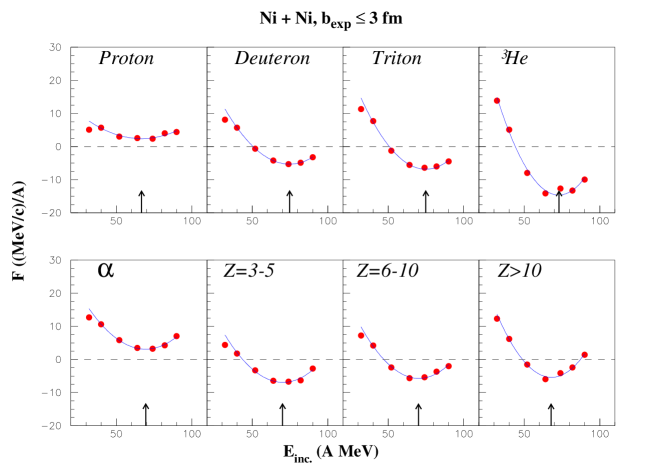
For the most central collisions (bexp 3 fm), the results are shown in figure 3 for the Ar + Ni system, in figure 4 for the Ni + Ni system and in figure 5 for the Xe + Sn system. In the first two experiments, the reaction plane was determined by using the momentum tensor method with the one plane per particle prescription. The flow parameter values has been determined by a linear fit in the Yr range from 0.4 to 0.6. The errors on flow parameter values have been estimated by changing the Yr range from 0.35 to 0.65 and from 0.45 to 0.55. The error bar do not appear on the figures when it is smaller that the symbol size.
The evolution of the flow parameter with the incident energy has a typical U shape for all particles. The incident energy which corresponds to the minimum flow value is located around 82 2 A.MeV for the Ar + Ni system and around 75 2 A.MeV for the Ni + Ni system. For both systems, these balance energies do not depend on the particle nature as for systems in reference [10]. They are in agreement with theoretical work [2]. These calculation were performed with K∞ 220 MeV and =0.8 , where is the free nucleon-nucleon cross-section.
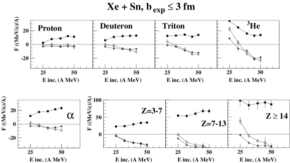
For the Xe + Sn system (figure 5), the results are shown for two reaction plane reconstruction procedures: the momentum tensor method (open diamonds) and the transverse momentum method (stars) with the one plane per particle prescription. As expected, both methods give close results. The U shape is barely seen for 3He and heavy particles (Z 3). For all particle types, the minimum flow energy is difficult to determine, since the flow parameter weakly depends on the incident energy. Unfortunately, the expected Ebal value is around 50 A.MeV which is the maximum incident energy available for this system. No accurate determination of Ebal can be done for this system. The full circles correspond to the momentum tensor method when one plane per event is determined. The flow parameter values are higher than the value obtained with one plane per particle due to the “auto-correlation” effect. The same behavior is observed with the lighter systems Ar + Ni and Ni + Ni when one plane per event is reconstructed.
But the most striking feature of figures 3, 4 and 5 for the one plane per particle prescription is the observation of negative flow parameter values for d, t, 3He and fragments with a charge greater than 3. By definition only positive values are expected. Negative flow parameter values have already been observed in previous studies [25] , but no clear explanation was given for this effect. We will propose in the next two sections two possible scenarios for these negative flow values.
IV The physical effect for negative flow values.
A possible explanation for the negative flow values is given by AMD calculations [11]: for light charged particles, the flow of promptly emitted (named “direct”) particles can be opposite to the flow of “evaporated” particles (emitted from the quasi-projectile QP and the quasi-target QT). By definition, the reaction plane is oriented positively in the mean direction of forward emitted products. Therefore, negative flow values can be measured.
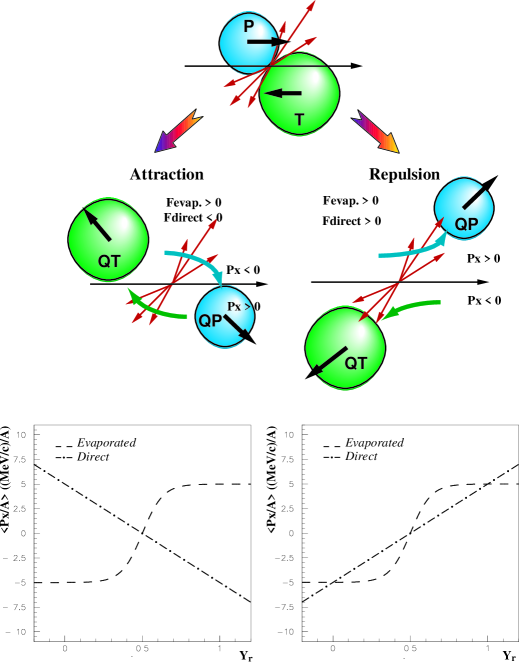
The direction of the “direct” flow in the reaction plane results mainly from screening effects. As shown in figure 6, in the first moments of the reaction, “direct” nucleons coming from the projectile (target) are screened by the target (projectile) nucleus. For a fixed impact parameter, the orientation of the “direct” flow is determined by the geometrical configuration at the touching point and is weakly dependent on the incident energy. It is always aligned on the same direction as the initial orientation of the projectile in the reaction plane. At variance, the direction of the “evaporated” flow is aligned on the final directions of the QP. This direction depends strongly on the incident energy, as it will been explained in the next paragraph. Experimental studies have shown that heavy fragments could be emitted by non-evaporative processes, like a neck break-up [26, 27, 28, 29, 30, 31, 32, 33, 34, 35, 36, 37]. Since the direction of emission of these fragments is mainly aligned on the QP-QT axis, their flow direction is identical to the so-called “evaporated” flow. The contribution of heavy fragments to the flow parameter will be always attributed to the “evaporated” component. If one assumes that the observed flow parameter results only from these two contributions, the evaporated and prompt emissions, a fairly simple picture can be proposed as shown in figures 6. The simple pictures shown here are for pedagogical purpose. They do not pretend to reproduce the true process. They are shown to give a feeling of what kind of physical effect could lead to the observation of negative flow parameter values.
At low incident energy, where the attractive part of the nucleon-nucleon interaction dominates, the QP and the QT are deflected to the opposite side relative to their initial directions (left column of figure 6). In this case, since Px /A is defined positive for particles which are deflected on the same side as the QP, the variation of Px /A with Yr is different for the two emissions: a “S” shape for the “evaporated” particles with a positive slope around mid-rapidity (dashed line in the lower left picture of figure 6) and a straight line with a negative slope for the “direct” particles (dashed and dotted line).
At higher energies, where the repulsive part on the interaction is dominant, the QP “bounces” on the QT (right column of figure 6). In this case, the variations of Px /A with Yr give a positive slope around mid-rapidity for the two emissions as shown in the lower right panel of figure 6. The observed variation of Px /A with Yr is a combination of these two contributions with their associated Yr distributions.
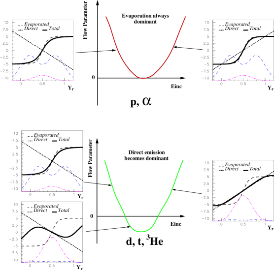
Such combinations are schematically shown in figure 7. For each side panel, the original Px /A evolution of the “direct” particles (straight dashed and dotted line) and its corresponding Yr distribution (dashed and dotted gaussian distribution) are plotted. The Px /A contribution (“S” shape) and the Yr distribution of “evaporated” particles (sum of two gaussian distributions) are plotted as dashed lines. The resulting evolution of Px /A corresponds to the thick line. It is simply obtained by summing the two Px /A contributions weighted by their corresponding Yr distributions.
If the contribution of “evaporated” particles is dominant, then the resulting flow parameter value is always positive (upper row of figure 7). The “S” shape is weakly affected by the contribution of “direct” emissions. At variance, if “direct” emissions become dominant (lower row of figure 7), then a negative flow value can be obtained. At low incident energies, the evolution of Px /A with Yr is dominated by the “evaporated” particles. When “direct” emissions becomes dominant, the evolution of Px /A with Yr follows the one of the “direct” particles, and the “S” shape is strongly deformed. Negative slopes can be found at mid-rapidity, i.e. negative flow parameter values.
This explanation is very tempting for the light charged particles. Deuterons, tritons and are predominantly emitted in the mid-rapidity regions, whereas protons and alpha particles are emitted as much by the QP and QT as by the mid-rapidity emissions [38, 39]. At the same time, positive flow values are measured for alpha and protons and negative values for deuterons, tritons and (see figures 3, 4 and 5). Both experimental features support the above interpretation. But this does not explain the negative values observed for the heavier fragments. Within the simple interpretation of sideward flow, the emission of fragments via cluster-cluster collisions of preexisting fragments in both partner bulk has a very low probability. As already mentioned, for PLF and the TLF, this observation is even in contradiction to the reaction plane orientation which is always oriented along the direction of the quasi-projectile. The solution of this puzzle has to be found elsewhere.
Previous studies [23] have shown that the reaction plane determination method and the associated issue of auto-correlations could strongly disturb the measurement of flow parameter. Before attributing the observation of negative flow parameter values to physical effects, one has first to be sure that these negative values are not due to the analysis methods. The next section is devoted to the test of reaction plane determination methods. The origins of the so called “auto-correlation” effects will also be studied.
V Test of the reaction plane determination methods
A Reaction plane estimation.
Let us now briefly describe three commonly used methods: the transverse momentum method [19], the momentum tensor method [20] and the azimuthal correlations method [21]. From now on, the axis is the beam axis, the axis is the axis in the reaction plane which is perpendicular to the beam axis and axis is the axis perpendicular to the reaction plane. The transverse momentum method, explained in details in [19], is based on the fact that the sum of transverse momenta of particles emitted by the quasi-projectile is opposite to the sum of the transverse momenta of particles emitted from the quasi-target . This is valid within the binary mechanism hypothesis, where the mid-rapidity contribution is negligible. Those vectors belong to the reaction plane. In order to maximize the efficiency of the method, one has to calculate the difference of the two vectors . Usually, is determined in the following way:
| (3) |
where is the total number of particles in the event, is the transverse momentum of particle and a weight defined as follows:
| (4) |
or
| (5) |
where is the reduced rapidity of the particle, the center of mass reduced rapidity (close to the reduced rapidity of the nucleon-nucleon frame for the symmetric systems) and a parameter which allows to remove the mid-rapidity particles from the estimation of the reaction plane. defines with the beam direction the reaction plane. With this definition, the reaction plane is systematically oriented along the quasi-projectile direction.
Another way to estimate the reaction plane is to calculate and diagonalize a tensor . The beam axis defines with the eigenvector corresponding to the highest eigenvalue the reaction plane. As for the transverse momentum the reaction plane is oriented along the direction of the quasi-projectile. The tensor is defined in the following way:
| (6) |
where is the momentum component along the axis () for the particle . is a weight which is usually set to the inverse of the mass of the particle (energy tensor).
The azimuthal correlations method is based on the following observation: in case of strong in-plane emission (high flow parameter value), the sum of the distances of particles momenta with respect to that plane are minimum [21]. This sum is calculated as follows:
| (7) |
where and are the transverse momentum components along the and axis respectively and , where is the angle of the reaction plane relative to the axis. Experimentally, one has to find the value of which minimizes . With this method, the orientation of the reaction plane is not defined. One has to use the transverse momentum method to find it. In case of strong out-of-plane particle emission ( squeeze-out), the estimated reaction plane angle is wrong by .
B Testing procedure
Since the flow parameter is obtained from the average value of the transverse momentum projection on the reaction plane, one has to rebuild this plane from the experimental data. We have checked the reliabilities of the three reaction plane reconstruction methods. The general procedure of the test is the following: a known flow parameter value is set for a sample of generated events; then the reaction plane estimation method is applied on that sample and the so called “experimental flow parameter” is determined. A method is considered effective if the experimental value is equal or close to the initial one . This allows to also check the additional disturbance introduced by the experimental set-up compared to the method itself.
To set the flow parameter value to an event, an in-plane component is added to the transverse momentum of each particle, similarly to the procedure used in [23]. The amplitude of this in-plane component depends on the reduced rapidity of the particle:
| (8) |
where is the flow parameter value to be set on, Yr is the reduced rapidity of the particle, its mass and the in-plane component.
The test has been performed on two systems Ar + Ni at 74 A.MeV and Xe + Sn at 50 A.MeV. These two systems have been studied with INDRA and their comparison allows to check the effect of the mass of the system on the transverse flow measurement. These energies values have been chosen because they are close to the expected balance energy. For each system, 15000 events have been generated using the SIMON code, whose entrance channel includes a pre-equilibrium emission of protons and neutrons [40]. SIMON is not used to reproduce the experimental data, but rather as an event generator. The goal is to check how the reaction plane reconstruction methods react in a well defined situation. In this test, only the most central collisions have been used. The flow parameters for the different particle types are not exactly zero but close to zero, and differ from a particle type to another. The effect of the addition of the component is to add the value of to the original value of the flow parameter, giving a value. This procedure will allow to study the effects of the different reaction plane reconstruction methods on flow parameters measurements, as in [23].
C One plane per event or one plane per particle?
Since the transverse momentum is used both for the reaction plane estimation and for the projection, auto-correlations are expected (see full circles in figures 1 and 2). Auto-correlation effects are also amplified by the loss of information due to a non perfect detection. The usual way to solve this problem is to remove the particle which has to be projected from the estimation of the reaction plane. Thus, an additional corrective component is added to the momentum of the remaining particles in order to ensure the conservation of the total momentum. Its definition is the following:
| (9) |
where is the removed particle, its velocity, the mass of particle () and the event multiplicity. In this case, one plane is determined for each particle of the event.
Two prescriptions have been used for the methods described in section V A. In the first one, one plane per event is determined. This allows to check the effect of the auto-correlations with respect to the method used. In the second one, one plane per particle is determined, in order to test the efficiency of the correction.
1 Azimuthal dispersion between the true reaction plane and the reconstructed one
To compare the relative efficiencies of these methods, the distribution of the angular azimuthal difference between the true and the reconstructed reaction plane directions has been studied. Such distributions have been already shown (see figure 6 of [6]).
The observed mean value is zero. The accuracy of the reaction plane determination is estimated with the standard deviation of these distributions as a function of the added flow parameter value . Figure 8 shows such evolutions of with . has been used instead of because the values are different from a particle type to another, whereas the same value has been added to all particles. The upper row corresponds to the Ar + Ni system, the lower row, to the Xe + Sn system. The left column correspond to the case when one plane per particle is determined and the right column to the one plane per event prescription. No significant difference is found between these two prescriptions. For all methods and systems, the dispersion decreases when increases. For small values, the different methods give slightly different results because the initial flow parameter is not zero. As expected, the reaction plane determination is more accurate in case of strong in-plane emission. For both systems, the transverse momentum method and the tensor method give similar accuracies, whereas for the azimuthal correlation method the dispersion is systematically higher for all values. For the Xe + Sn system, the values of are smaller than for the Ar + Ni system.
From these observations, three main conclusions can be drawn: i) the azimuthal dispersion of the reconstructed reaction plane is the same for the one plane per particle and one plane per event prescriptions; ii) similarly to the conclusion of reference [6], the azimuthal correlation method is less accurate than the two other methods, even at low values; iii) the higher the mass of the system and the higher the value, the more accurate is the reaction plane reconstruction.
Surprisingly, no difference is seen on between the one plane per particle and the one plane per event prescriptions, whereas strong discrepancies are seen for the Px /A =f(Yr ) curves (figures 1 and 2). One has to keep in mind that in the present case, only the deviation from the true reaction plane is studied. For the Px /A =f(Yr ) curves, the combined effects of the reaction plane reconstruction accuracy and of the projection of transverse momenta on the reconstructed reaction plane are present.
2 Measured flow parameter versus initial flow parameter
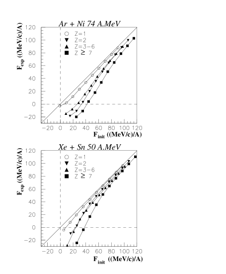
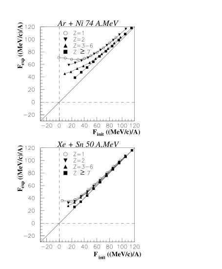
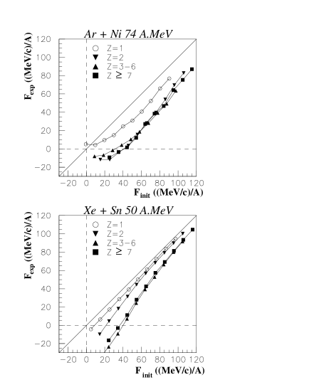
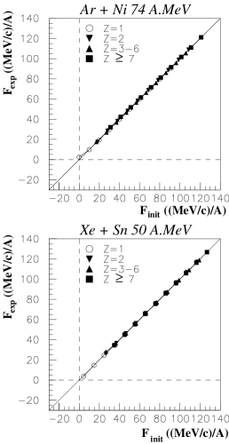
For the transverse momentum method, the dependence of on the initial value of the flow parameter is shown in figure 9 in the case of one plane per particle (left column) and in case of one plane per event (right column). For one plane per particle, the procedure used to remove auto-correlations seems to be efficient for isotopes. For heavier particles, is systematically below . This underestimation increases with increasing charge. For a given value, the underestimation is lower for Xe+Sn system than for Ar+Ni. Finally, the amplitude of this underestimation decreases with increasing value of .
With one plane per event (right column of figure 9), values are systematically larger than values due to the auto-correlation effects mentioned above. For a fixed value, the overestimation increases with decreasing charge of the particle. Here again, the amplitude of the overestimation diminishes for higher values of and with increasing mass of the system.
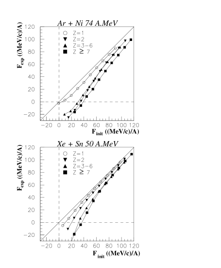
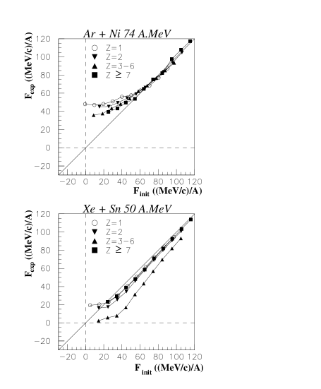
For the momentum tensor method, results are shown in figure 10 for one plane per particle (left column) and for one plane per event (right column). The same trends are observed as for the transverse momentum method. The auto-correlation effects are smaller in the case of one plane per event.
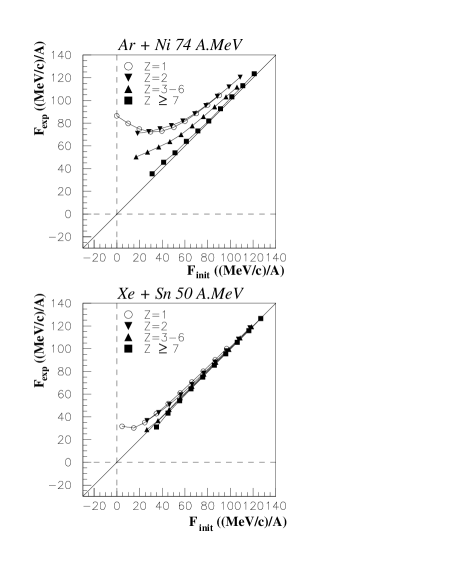
For the azimuthal correlation method (figure 11), the same trends are observed as for the two other methods. The main difference is a somewhat larger underestimation of the flow parameter value.
3 Influence of the experimental set-up
Part of the anti or auto correlation may be related to the detector efficiency. In order to probe the effect of the experimental set-up, the INDRA “filter” has been applied on the generated events. The INDRA “filter” is a sophisticated software which simulates the response of the detector. For each particle, the energy losses in each layer of the detector are calculated. An identification procedure similar to the experimental one is then applied on the energy losses giving back the charge and the energy of the detected particle. Doing this, multiple hits in a detector are treated in the same way they are treated in the experiment. This procedure allowed to reproduce the angular and energy thresholds observed experimentally.
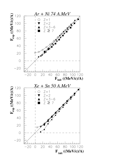
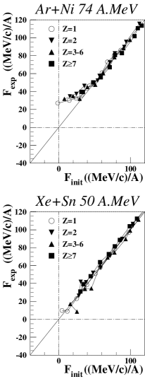
The reaction plane is then reconstructed from the so called “filtered” events. In figure 12, the correlation between and is plotted for the momentum tensor method with the one plane per event prescription. For the two systems studied here, the results are very similar to those obtained with a perfect detection (see the right column of figure 10). The measured flow values are above the initial ones for the Ar + Ni system, and close to the initial ones for the Xe + Sn system. The detector has a weaker effect than the reaction plane determination procedure. This conclusion is identical to those made in reference [23] for a array which had higher thresholds.
4 Conclusions of the simulations
The following conclusions can be drawn from the previous study:
i) removing the particle of interest from the reaction plane
introduces an anti-correlation
which is not counterbalanced by adding a corrective momentum
to the momentum of other particles. The
anti-correlation effect leads to an underestimation of sideward flow values;
ii) when one plane per particle is determined,
the amplitude of the anti-correlation is higher for small values, for
heavy particles and for small system size;
iii) when one plane per event is determined,
the amplitude of the auto-correlation is higher for small values, for
light particles and for small system size;
iv) for all methods, for the one plane per event prescription,
the auto-correlation effect leads to an overestimation of the flow
parameter value.
This overestimation is minimum for the momentum tensor method;
v) the best results are obtained for the momentum tensor method
with the one plane per event prescription;
vi) Detection effects are weaker than effects induced by the
procedures used to reconstruct the reaction plane.
One could conclude from these simulations that the best method to measure small sideward flow values is the momentum tensor method with one plane per event. Unfortunately, the simulation is too simple compared to the experimental situation. We remind the reader that in this simulation, the mid-rapidity contribution is only present for protons and neutrons. This is why the “auto-correlation” effect is mainly seen for protons in the simulation. In the experimental data, the mid-rapidity emission is also made of heavier particles [38, 39]. The autocorrelation effect is seen for all particles for the Ar + Ni system (full circles in figures 1 and 2) as well as for the Xe + Sn system (full circles in figure 5). In the latter case, the flow parameter is weakly dependent on the incident energy. Therefore, from the experimental results, it turns out that the “auto-correlation” effects are strong. In other words, qualitative effects may be understood thanks to the simulations but quantitative estimations of the corrections required in the data are difficult to realize from these simulations. Such a correction may be done if the “auto-correlation” effect is well understood. The study of the origins of the “auto-correlation” effect is done in the next section.
D Origin of the auto-correlations
These studies show us that the methods developed at high energies, where high values of sideward flow are measured, are not well suited for intermediate energies where the flow parameter values are typically around or below 30 MeV/c/A. The amplitude of the anti or auto correlations depends also on the nature of the particle. Let us try nevertheless to identify the origin of the auto-correlations at intermediate energies.
First of all, one has to make some remarks. If a method would be able to reconstruct perfectly the reaction plane from the momentum of all particles, no auto-correlation effect would be seen. This is shown for example in the right column of figure 10 for the Xe+Sn system. The experimental flow parameter is very close to for values above 20 MeV/c/A, although the momenta of all particles have been used to calculate the momentum tensor. This is quite unexpected since for high values, the transverse momenta values are large. The auto-correlation effect should be maximum for high . The usual explanation of the auto-correlation effect does not seem to be the right one. If so, where does this “auto-correlation” effect come from ? Since the azimuthal correlation method is less accurate than the two other ones, the origin of the “auto-corellations” will not be checked for this method.
1 “Auto-correlations” for the transverse momentum method
In the transverse momentum method, one assumes that the particles emitted above Ycm are all coming from the decay of the quasi-projectile (QP), and those emitted below Ycm are all coming from the decay of the quasi-target (QT). But at intermediate energies, the contributions from the QT, the QP and from the mid-rapidity area are mixed, especially for the most violent collisions [38, 39]. In addition, for the most central collisions, the azimuthal angular distributions are rather flat and no privileged direction can be clearly seen. Therefore a wrong weight may be attributed to the particles, and the estimated reaction plane may have nothing to do with the true one. In this case, the reconstructed reaction plane may be oriented along the particles with the highest momenta.
On the other hand, if the right weight was attributed to the right particles, this effect should vanish. This can be checked in the simulation, for which the origin of particles is known. The results are shown in figure 13. In this simulation, a pure binary scenario has been assumed: the first stage of the collision leads to the formation of a quasi-projectile and a quasi-target both deflected in the reaction plane, without any pre-equilibrium emissions. One plane per event is determined, using the transverse momentum method, and the weight of the particles is attributed according to their origin: +1 for the particles emitted by the quasi-projectile, -1 for those emitted by the quasi-target. It is seen that the effect of “auto-correlation” is removed, even for the smaller flow values. The so called “auto-correlation” effect comes from a loss of information (the origin of the detected particles), instead of the use of the transverse momenta in both the reaction plane determination and in the projection.
In the experiment, the exact knowledge of the origin of the particle is impossible, especially for the most damped reactions. In addition the collisions are not purely binary due to prompt emissions. The promptly emitted particles carry a part of the total tansverse momentum and the QP and QT are hence pushed out of the reaction plane. In the experiment, the perfect determination of the reaction plane using the tranverse momentum method is very difficult, especially for the central collisions.
2 “Auto-correlations” for the momentum tensor method
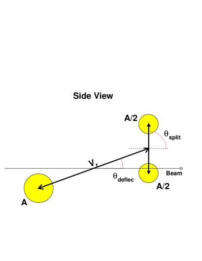
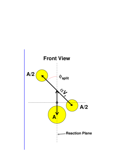
For the momentum tensor method, the origin of “auto-correlations” effects can be understood using a simple test. Let us consider the case where a quasi-projectile of mass number splits into two equal size fragments and the quasi-target of the same mass number remains unchanged. The quasi-projectile and the quasi-target are deflected in the reaction plane. The axis joining their center of mass has an angle with respect to the beam axis (see figure 14). The axis joining the two fragments issued from the splitting of the quasi-projectile has an angle with respect to the beam direction and an angle with respect to the reaction plane. The relative velocity between the quasi-projectile and the quasi-target is and the relative velocity between the two fragments of the quasi-projectile is . A scheme of the described configuration is presented in figure 14.
The momentum tensor of such a simple case can be calculated and one can study the azimuthal angular difference between the reconstructed reaction plane and the true one. The direction of the reaction plane is defined in the plane transverse to the beam axis, displayed in the right panel of figure 14. In this panel, the QT is by definition in the reaction plane but the two splitting fragments are out of the plane.
The first key variable is . When its value is small (close to zero), the QP-QT axis is obviously the main axis and the reaction plane is perfectly determined. But when the value is big enough the axis between the two splitting fragments may become the main axis. In this case, the reconstructed reaction plane direction may be dependent on the splitting direction which is the second key variable.
In figure 15, the evolutions of as a function of and are displayed. The angles and are set respectively to 10∘ and 40∘ . Similar pictures are obtained for other and values. For large enough values of is strongly dependent on . For low values of , i.e. small relative velocities of the two fragments compared to the relative velocities of the quasi-projectile and the quasi-target, does not depend on and is equal to zero. The two out-of-plane fragments do not introduce much pertubations on the reconstruction procedure. The direction of the reconstructed reaction plane is mainly determined by the QT. The reaction plane is therefore well estimated. On the other hand, when is larger than 1, the reaction plane is mainly determined by the two out-plane fragments. The direction of the reconstructed reaction plane is therefore correlated to the splitting direction. In the experiment, this last configuration is similar to the most violent (central) collisions but with a larger multiplicity.
If the two fragments issued from the splitting of the quasi-projectile were gathered before applying the momentum tensor method, the reaction plane would be perfectly determined whatever the fragmenting configuration. That means that if the origin of the fragments is known, on can determine perfectly the reaction plane by grouping the fragments coming from the same source in a single fragment. The results of the momentum tensor method depend on the way the fragments are gathered. As for the tranverse momentum method, a perfect determination of the reaction plane by using the momentum tensor method is very difficult in the experiment.
E Discussion
For incident energies around the balance energy, the standard methods used for the reaction plane reconstruction are not well suited. Whatever the method used, the one plane per event prescription leads to an “auto-correlation” effect i.e. a large overestimation of the flow parameter values. At variance, the one plane per particle prescription induces an anti-correlation effect which gives an underestimation of the flow parameter.
This indicates that the negative flow values observed in experimental data can be attributed to the used reconstruction methods, especially for the heaviest fragments. For the light charged particles, the physical effect can not be completely ruled out, since positive values of flow are observed for alphas, whereas negative values are expected if the reaction plane determination methods effects are dominant. For such particles, the two effects are probably mixed and more detailed studies have to be performed to establish their relative weights in the observed values. To obtain the true flow parameter values, one has to understand the auto-correlation effects in order to correct them accurately.
But understanding the origin of the “auto-correlation” effects is a complicated task. To correct them, a complete knowledge of the origin of particles is needed. This can be achieved only for the less violent collisions and/or at higher energies where the mixing between the different contributions is weak. For the most violent collisions, such a knowledge is unreachable unless assumptions are made. But in this case, the flow values obtained may only result from these assumptions.
Since the correction of experimental data seems to be impossible, it could be easier to apply the experimental filter and the analysis procedure on theoretical calculations. Most of the available dynamical calculations have to evolve to enable this procedure, since most of them are following the time evolution of the one body density. More precisely, the dynamical calculations should include the proper description of particle and fragment formation.
VI Conclusions
The in-plane flow parameter has been determined for the Ar + Ni collisions from 32 A.Mev to 95 A.Mev, for the Ni + Ni system from 32 A.Mev to 90 A.MeV and for the Xe + Sn system from 25 A.MeV to 50 A.MeV. For central collisions, the balance energies are equal to 82 2 A.MeV for the Ar + Ni system and 75 2 A.MeV for the Ni + Ni system. For the Xe + Sn system, the balance energy is around 50 A.MeV, but experiments at higher incident energies have to be performed to confirm the result. These values are in agreement with the systematics of balance energies found in other experiments. This systematics has been reproduced by a dynamical model assuming K∞ 220 MeV and =0.8 [2]. As already observed, the balance energy weakly depends on the particle nature. For these central collisions, negative flow values are observed for both systems. Two different explanations are proposed for these negative values.
The first one, supported by transport model calculations, attributes this effect to the relative importance between the prompt emission and the evaporative one. A negative flow parameter value can be observed if the prompt emission is dominant. This explanation seems to be satisfactory for the light particles. Deuterons, tritons and are predominantly emitted in the mid-rapidity regions [38, 39] and their flow parameter values are indeed negative. At variance, for protons and alpha particles, the measured flow parameters are positive. They are emitted as much by the QP and QT as at mid-rapidity. But on the other hand, negative flow values are measured for fragments while the prompt emission is not the dominant process for these products. For these heavy fragments, the observed negative values cannot be explained in this way.
The second explanation attributes these negative values to the experimental methods used to extract the reaction plane. The usual method used to avoid auto-correlations, the omission of the particle of interest, leads to an anti-correlation. This induces an inversion of the reaction plane reaction and then lead to the measurement of negative flow values. The amplitude of this effect increases when the flow parameter value decreases i.e. when the incident energy is getting closer to the balance energy. This explanation is supported by the observation of negative flow values for the heaviest fragments, whereas a positive value is expected. A careful study of the “auto-correlation” effect shows that its manifestation results from the loss of information about the product origins for both methods.
In experimental data, these two effects are probably mixed up. They disturb the measurement of the absolute value of sideward flow, especially around the balance energy for which low flow parameter values are expected. On the other hand, the relative evolutions with incident energy, and especially the determination of the balance energy, are in agreement with previous experimental studies and theoretical calculations. It may indicate a relative robustness of the balance energy variable. In the present status, the real effect can only be studied with simulations on which the complete experimental procedure can be applied. An accurate determination of the in-medium nucleon-nucleon interaction parameters can only be achieved if the disturbances induced by the analysis methods and the experimental set-up are explicitely taken into account. This requires an evolution of dynamical calculation to make possible this comparison procedure.
REFERENCES
- [1] G.F.Bertsch, W.G.Lynch and M.B.Tsang, Phys. Let. B189 , 384 (1987).
- [2] V.De La Mota, F.Sébille, M.Farine, B.Remaud and P.Shuck, Phys. Rev. C 46 , 677 (1992).
- [3] G.D.Westfall et al., Phys. Rev. Let. 71 , 1986 (1993).
- [4] W.Q.Shen et al., Nucl. Phys. A551 , 333 (1993).
- [5] R.Popescu et al., Phys. Let. B331 , 285 (1994).
- [6] J.C.Angélique et al., Nucl. Phys. A614 , 261 (1997).
- [7] D.J.Magestro, W.Bauer and G.D.Westfall, Phys. Rev. C 62 , 041603 (2000).
- [8] J.J.Molitoris, H.Stöcker and B.L.Winer, Phys. Rev. C 36 , 220 (1987).
- [9] H.M.Xu, Phys. Rev. Let. 67 , 2769 (1991).
- [10] G.D.Westfall, Nucl. Phys. A630 , 27c–40c (1998).
- [11] A.Ono and H.Horiuchi, Phys. Rev. C 51 , 299 (1995).
- [12] B.Li, Z.Ren, C.M.Ko and S.J.Yennello, Phys. Rev. Let. 76 , 4492 (1996).
- [13] R.Pak et al., Phys. Rev. Let. 78 , 1022 (1997).
- [14] W. Reisdorf, Nucl. Phys. A630 , 15c–26c (1998).
- [15] J.Pouthas et al. (INDRA Collaboration), Nucl. Inst. and Meth. A357 , 418 (1995).
- [16] J.Pouthas et al., Nucl. Inst. and Meth. A369 , 222 (1996).
- [17] J.C.Steckmeyer et al., Proceedings of the XXXIII International Winter Meeting on Nuclear Physics, Bormio, Italy, Edited by I.Iori, 255 (1995).
- [18] J.Péter et al., Nucl. Phys. A519 , 611 (1990).
- [19] P.Danielewicz et al., Phys. Rev. C 38 , 120 (1988).
- [20] J.Cugnon and D.L’Hote, Nucl. Phys. A397 , 519 (1983).
- [21] W.K.Wilson et al., Phys. Rev. C 41 , 1881 (1990).
- [22] C.A.Ogilvie et al., Phys. Rev. C 40 , 2592 (1989).
- [23] J.P.Sullivan et al., Phys. Let. B249 , 8 (1990).
- [24] C.A.Ogilvie et al., Phys. Rev. C 42 , R10 (1990).
- [25] D.Krofcheck et al., Phys. Rev. C 46 , 1416 (1992).
- [26] R.Bougault et al., Nucl. Phys. A488 , 255 (1989).
- [27] L.Stuttgé et al., Nucl. Phys. A539 , 511 (1992).
- [28] J.F.Lecolley et al., Phys. Let. B354 , 202 (1995).
- [29] Y.Larochelle et al., Phys. Rev. C 59 , 565 (1999).
- [30] J.F.Dempsey et al., Phys. Rev. C 54 , 1710 (1996).
- [31] J.Tõke et al., Nucl. Phys. A583 , 519 (1995).
- [32] S.L.Chen et al., Phys. Rev. C 54 , 2114 (1996).
- [33] C.P.Montoya et al., Phys. Rev. Let. 73 , 3070 (1994).
- [34] J.Lukasik et al. (INDRA Collaboration), Phys. Rev. C 55 , 1906 (1997).
- [35] G.Casini et al., Phys. Rev. Let. 71 , 2567 (1993).
- [36] A.A.Stefanini et al., Zeit. Phys. A351 , 167 (1995).
- [37] F.Bocage et al. (INDRA Collaboration), Nucl. Phys. A676 , 391 (2000).
- [38] T.Lefort et al. (INDRA Collaboration), Nucl. Phys. A662 , 397 (2000).
- [39] D.Doré et al. (INDRA Collaboration), Phys. Rev. C 63 , 034612 (2001).
- [40] D.Durand, Nucl. Phys. A541 , 266 (1992).