Directed and elliptic flow of charged pions and protons in Pb + Pb collisions at 40 and 158$A$ GeV

Abstract

Directed and elliptic flow measurements for charged pions and protons are reported as a function of transverse momentum, rapidity, and centrality for 40 and 158$A$ GeV Pb + Pb collisions as recorded by the NA49 detector. Both the standard method of correlating particles with an event plane, and the cumulant method of studying multiparticle correlations are used. In the standard method the directed flow is corrected for conservation of momentum. In the cumulant method elliptic flow is reconstructed from genuine 4, 6, and 8-particle correlations, showing the first unequivocal evidence for collective motion in A+A collisions at SPS energies.

I Introduction

In non-central collisions, collective flow leads to characteristic azimuthal correlations between particle momenta and the reaction plane. The geometry of a non-central collision between spherical nuclei is uniquely specified by the collision axis and the impact parameter vector ${\bf b}$. In particular, the latter defines a unique reference direction in the transverse plane. Directed flow ($v_{1}$) and elliptic flow ($v_{2}$) cause correlations between the momenta of outgoing particles with this reference direction VoZh96 . They are defined by

$$v_{1}\equiv\left\langle\cos(\phi-\Phi_{RP})\right\rangle,\ \ v_{2}\equiv\left\langle\cos(2(\phi-\Phi_{RP}))\right\rangle,$$ (1)

where $\phi$ denotes the azimuthal angle of an outgoing particle and $\Phi_{RP}$ is the azimuthal angle of ${\bf b}$. Angular brackets denote an average over particles and events.

Since primary collisions between the incoming nucleons are expected to be insensitive to the direction of impact parameter at high energy, azimuthal correlations are believed to result from secondary interactions, or final state interactions. As such, they are sensitive probes of “thermalization,” which should be achieved if final state interactions are strong enough. In the energy regime in which relatively few new particles are created, the flow effects are due to the nucleons which participate in the collision. Thus at low energy flow is used to study the properties of compressed nuclear matter and more specifically the nuclear equation of state WRHR . In nuclear collisions at ultrarelativistic energies the number of newly created particles is so large that their behavior will dominate the observable flow effects.

For the interpretation of experimental results on flow, theoretical tools are needed. There are two types of models to describe final state interactions, based either on hydrodynamics or on a microscopic transport (or cascade) approach. Hydrodynamics is adequate when the mean free path of particles is much smaller than the system size. Then, the interactions between the various particles in the system can be expressed in terms of global thermodynamic quantities, i.e., an equation of state. In this essentially macroscopic description, the collective motion results from a pressure gradient in the reaction volume, the magnitude of which depends upon the compressibility of the underlying equation of state OL92 . Since partonic and hadronic matter are expected to have different compressibilities, it may be possible to deduce from a flow measurement whether it originates from partonic or hadronic matter, or from the hadronization process taking place during the transition between the two WRHR ; DR96 ; OL98 ; PD99 . Microscopic cascade models are more appropriate when the mean free path of the particles is of the same order, or larger, than the size of the system, which is often the case in heavy ion collisions. They require a more detailed knowledge of the interactions (cross sections, etc.) of the various particles in the medium. Detailed flow analyses may help to falsify or confirm the corresponding model assumptions.

In particular, the study of the energy dependence of flow is considered Kolb:99 ; Kolb:00 ; Teaney:01 as a promising strategy in the search for evidence for the hypothesis that the onset of deconfinement occurs at low SPS energies. More generally, the energy scan project NA49-ADD1 at the CERN Super Proton Synchrotron (SPS) was dedicated to the search for the onset of deconfinement in heavy ion collisions. In fact anomalies observed in the energy dependence of total kaon and pion yields NA49-energy can be understood as due to the creation of a transient state of deconfined matter at energies larger than about 40$A$ GeV Gazdzicki:99 .

In that context, this paper presents the most detailed analysis so far of directed and elliptic flow of pions and protons at various SPS energies. The first publication from NA49 on anisotropic flow NA49PRL was based on a small set of 158$A$ GeV data with a medium impact parameter trigger with only the tracks in the Main TPCs used in the analysis. Subsequently a method was found for improving the second harmonic event plane resolution and revised results were posted on the web NA49Web . The present analysis of 158$A$ GeV data is both more detailed and more accurate than the previous one: it uses much larger event statistics, a minimum bias trigger, integration over transverse momentum $p_{t}$ or rapidity $y$ using cross sections as weights, and improved methods of analysis. Moreover, in this paper the NA49 results on flow at 40$A$ GeV are published for the first time. Preliminary results from this analysis have been presented in Refs. NA49QM99 ; Wetzler:QM02 ; Borghini:QM02 .

Two types of methods are used in the flow analysis: the so-called “standard” method Danielewicz:hn ; Ollitrault:1997di ; Poskanzer:1998yz requires for each individual collision an “event plane” which is an estimator of its reaction plane. Outgoing particles are then correlated with this event plane. This method, however, neglects other sources of correlations: Bose-Einstein (Fermi-Dirac) statistics, global momentum conservation, resonance decays, jets, etc. The effects of these “nonflow” correlations may be large at the SPS, as shown in Ref. Dinh:1999mn ; Borghini:2000cm . The standard method has been improved to take into account part of these effects. In particular, correlations from momentum conservation are now subtracted following the procedure described in Ref. Borghini:2002mv . Recently, a new method has been proposed which allows to get rid of nonflow correlations systematically, independent of their physical origin Borghini:2000sa ; Borghini:2001vi ; Borghini:2002vp . This method extracts directed and elliptic flow from genuine multiparticle azimuthal correlations, which are obtained through a cumulant expansion of measured multiparticle correlations. The results obtained with both methods will be presented and compared.

The paper is organized as follows: Sec. II covers the experiment, Sec. III describes the data sets, the selection criteria for events and particles, and the acceptance of the detector, in Sec. IV the two methods of flow determination are explained, and Sec. V contains the results on elliptic and directed flow as function of centrality and beam energy. Sec. VI focuses the discussion on model calculations and Sec. VII summarizes the paper.

II Experiment

The NA49 experimental set–up na49_nim is shown in Fig. 1. It consists of four large-volume Time Projection Chambers (TPCs). Two of these, the Vertex TPCs (VTPC-1 and VTPC-2), are placed in the magnetic field of two super-conducting dipole magnets (VTX–1 and VTX–2). This allows separation of positively and negatively charged tracks and a precise measurement of the particle momenta ($p$) with a resolution of $\sigma(p)/p^{2}\cong(0.3-7)\cdot 10^{-4}$ (GeV/$c$)^-1. The other two TPCs (MTPC-L and MTPC-R), positioned downstream of the magnets, were optimized for high precision detection of the ionization energy loss $dE/dx$ (relative resolution of about 4%) which provides a means to measure the particle mass. The TPC data yield spectra of identified hadrons above midrapidity. The magnet settings at 158$A$ GeV were: $B$(VTX–1) $\cong$ 1.5 T and $B$(VTX–2) $\cong$ 1.1 T. In order to optimize the NA49 acceptance at 40$A$ GeV the magnetic fields of VTX–1 and VTX–2 were lowered in proportion to the beam momentum. Data were taken for both field polarities.

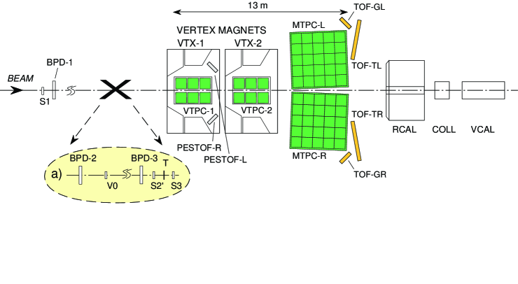
Figure 1: (Color online) The experimental set–up of the NA49 experiment na49_nim .

The target (T), a thin lead foil (224 mg/cm², approx. 0.47% of Pb-interaction length), was positioned about 80 cm upstream from VTPC–1. Beam particles were identified by means of their charge as seen by a gas Cherenkov counter (S2’) in front of the target. An identical veto-counter directly behind the target (S3) is used to select minimum bias collisions by requiring a reduction of the Cherenkov signal by a factor of about 6. Since the Cherenkov signal is proportional to $Z^{2}$, this requirement ensures that the projectile has interacted with a minimal constraint on the type of interaction. This limits the triggers on non-target interactions to rare beam-gas collisions, the fraction of which proved to be small after cuts, even in peripheral Pb+Pb collisions. The counter gas which is present at atmospheric pressure all the way from S2’ to the target and further on to S3 was He for the 158$A$ GeV and CO₂ for the 40$A$ GeV runs. The signal from a small angle calorimeter (VCAL), which measured the energy carried by the projectile spectators, was used to make off-line centrality selections. The geometrical acceptance of the VCAL calorimeter was adjusted for each energy in order to cover the projectile spectator region by a proper setting of a collimator (COLL) na49_nim ; veto . The NA49 coordinate system is defined as right handed with the positive $z$-axis along the beam direction and the $x$-axis in the horizontal and the $y$-axis in the vertical plane.

III Data

The data on Pb+Pb collisions at 40$A$ GeV were collected within the energy scan program at the CERN SPS NA49-ADD1 . As part of this program Pb+Pb collisions at 20, 30, 40 and 80$A$ GeV were recorded by the NA49 detector during heavy ion runs in 1999, 2000 and 2002. Due to limited beam time, minimum bias data required for a flow analysis were not taken at 80 $A$ GeV, and the 20 and 30 $A$ GeV data from 2002 have not yet been analyzed. The corresponding data at the top SPS energy (158$A$ GeV) were taken from runs in 1996 and 2000.

III.1 Data sets

The data sets used in this analysis were recorded at 158$A$ GeV and 40$A$ GeV with a minimum bias trigger allowing for a study of centrality and energy dependence. Since central collisions have a small weight in such a selection of events, their number was augmented by data from central trigger runs at 158$A$ GeV. The final results for the 40$A$ GeV beam minimum bias data were obtained from 350 k minimum bias events for the standard method and 310 k events for the cumulant method. For the 158$A$ GeV results, the minimum bias events used were 410 k for the standard method and 280 k for the cumulant method. The 12.5% most central events added in were 130 k for the standard method and 670 for the cumulant method. In addition, for the integrated cumulant results, 280 k events from another run triggered on 20% most central collisions was added. These numbers refer to events which fulfill the selection criteria. After verifying that the analysis of events recorded with opposite field polarities give compatible results the corresponding data sets were combined and processed together. Full coverage of the forward hemisphere for pions and protons is achieved by using the tracks combined from both the Vertex and Main TPCs.

III.2 Selections and particle identification

The sample of events provided by the hardware trigger is contaminated by non-target interactions which are removed by a simultaneous cut on the minimum number of tracks connected to the reconstructed primary vertex (10) and on the deviation from its nominal position in space (0.5 cm in all dimensions). Quality criteria ensured that only reliably reconstructed tracks were processed. This acceptance was defined by selecting tracks in each TPC if the number of potential points in that TPC based on the geometry of the track was at least 20 in the vertex TPCs and 30 in the main TPC. In order to avoid split tracks the number of fit points for the whole track had to be greater than 0.55 times the number of potential points for that track. The $\chi^{2}$ per degree of freedom of the fit had to be less than 10. Tracks with transverse momentum ($p_{t}$) up to 2 GeV/$c$ were considered. The fraction of tracks of particles from weak decays or other secondary vertices was reduced by cutting on the track distance from the reconstructed event vertex in the target plane ($\pm$3 cm in the bending and $\pm$0.5 cm in the non-bending direction).

The binning of the event samples in centrality was done on the basis of the energy measurement in the forward calorimeter (VCAL). Its distribution was divided into 6 bins with varying widths. Each bin has a mean energy ($E^{0}$) and corresponds in a Glauber-like picture to an impact parameter range ($b$) with an appropriate mean, a mean number of wounded nucleons $\left\langle N_{WN}\right\rangle$, a mean number of participants $\left\langle N_{part}\right\rangle$, and a cross section fraction $\sigma/\sigma_{T}$ with $\sigma_{T}$ being the total hadronic inelastic cross section of Pb+Pb collisions which has been estimated to be 7.1 b at both energies. Details of the binning are given in Table 1. In the graphs “central” refers to bins 1 plus 2, “mid-central” to bins 3 plus 4, and “peripheral” to bins 5 plus 6. When we integrate over the first five centrality bins to present “minimum bias” results, we believe we have integrated out to impact parameters of about 10 fm corresponding to $\sigma/\sigma_{T}$=0.435.

In the standard method of flow analysis the determination of the event plane is required (see below). The uncertainty of its azimuthal angle in the laboratory coordinate system depends not only on the total number of particles used but also on the size and sign of the flow signal of these particles, which are in general different for different types of flow and different phase space regions. To optimize the resolution of the event plane orientation the following selection of tracks used for the event plane determination was made using $y$ in the center of mass and $p_{t}$. For the first harmonic: $0<p_{t}<1$ GeV/$c$ (centrality bins 3–6), $0<p_{t}<0.3$ GeV/$c$ (centrality bin 1), $0<p_{t}<0.6$ GeV/$c$ (centrality bin 2), $1.1<y<3.1$ for 158$A$ GeV data, and $0<p_{t}<1$ GeV/$c$ (centrality bins 1–6), $0.8<y<2.8$ for 40$A$ GeV data. For the second harmonic: $0<p_{t}<1$ GeV/$c$, $-0.5<y<2.1$ for 158$A$ GeV data, and $0<p_{t}<1$ GeV/$c$, $-0.4<y<1.8$ for 40$A$ GeV data. In comparison to these selections for good event plane resolution, the differential data to be presented go to higher $p_{t}$ but lower maximum $y$ values.

Particle identification is based on energy loss measurements ($dE/dx$) in the time projection chambers. An enriched sample of pions is obtained by removing those particles which are obviously not pions by appropriate cuts in the lab momentum - $dE/dx$ plane. The remaining contamination amounts to less than 5% for negatively charged pions. For positively charged pions it is less than 20% between 2 and 20 GeV/c momentum in the laboratory. Outside this range the contamination increases up to 35% for lower momenta. For higher momentum the contribution to the measured flow is small due to the vanishing cross section of pions in this region. Although the fraction of misidentified particles is substantial, the effect on the results will be small, since $v_{2}$ for pions and protons is comparable and depends on rapidity and $p_{t}$ in a similar way. The kaons are expected to follow the same trend. To examine the influence of the contamination, $v_{1}$ and $v_{2}$ of all charged particles were analyzed and compared to results for pions. The small differences are included in the quoted systematic errors. The proton identification is restricted to laboratory momenta above 3 GeV/$c$ and thus to the region of the relativistic rise of the specific energy loss. Tight upper limits of $dE/dx$ remove almost quantitatively all lighter particles. The remaining contamination amounts to less than 5% kaons and pions for 158$A$ GeV data and less than 8% for 40$A$ GeV data.

Table 1: Listed for the two beam energies and six centralities are: $E^{0}/E^{0}_{beam}$, the forward calorimeter energy divided by the beam energy; $\left\langle E^{0}/E^{0}_{beam}\right\rangle$, the mean value; $\sigma/\sigma_{T}$, the fraction of the total cross section in that bin; the integral of $\sigma/\sigma_{T}$; $b$, the estimated range of impact parameters; $\left\langle b\right\rangle$, the estimated mean impact parameter; $\left\langle N_{WN}\right\rangle$, the estimated number of wounded nucleons, and $\left\langle N_{part}\right\rangle$, the estimated mean number of participants. The 6 bins in centrality have different values of $E^{0}/E^{0}_{beam}$ at 40 and 158$A$ GeV since the acceptance of the forward calorimeter depends on beam energy.

Centrality	Central		Mid-Central		Peripheral
	Minimum Bias
Centrality bin	1	2	3	4	5	6
158$A$ GeV = 32.86 TeV
$E^{0}/E^{0}_{beam}$	0 - 0.251	0.251 - 0.399	0.399 - 0.576	0.576 - 0.709	0.709 - 0.797	0.797 - $\infty$
$\left\langle E^{0}/E^{0}_{beam}\right\rangle$	0.19	0.32	0.49	0.65	0.75	0.86
40$A$ GeV = 8.32 TeV
$E^{0}/E^{0}_{beam}$	0 - 0.169	0.169 - 0.314	0.314 - 0.509	0.509 - 0.66	0.66 - 0.778	0.778 - $\infty$
$\left\langle E^{0}/E^{0}_{beam}\right\rangle$	0.12	0.24	0.41	0.58	0.71	0.86
both energies
$\sigma/\sigma_{T}$ in each bin	0.050	0.075	0.11	0.10	0.10	0.57
${\rm Sum}~{}\sigma/\sigma_{T}$	0.050	0.125	0.235	0.335	0.435	1.00
$b$ (fm)	0 - 3.4	3.4 - 5.3	5.3 - 7.4	7.4 - 9.1	9.1 - 10.2	10.2 - $\infty$
$\left\langle b\right\rangle$ (fm)	2.4	4.6	6.5	8.3	9.6	11.5
$\left\langle N_{WN}\right\rangle$	352	281	204	134	88	42
$\left\langle N_{part}\right\rangle$	366	309	242	178	132	85

III.3 Acceptance

The NA49 detector was designed for large acceptance in the forward hemisphere of the center-of-mass frame. The resulting acceptance is illustrated by the density distributions of protons and pions as a function of rapidity and transverse momentum as seen in Ref. NA49-energy . The scaling of the magnetic field strength with beam energy ensures similar distributions at both energies. The NA49 detector employs two dipole magnets with main field components perpendicular to the beam axis. This breaking of rotational symmetry together with the rectangular TPC shapes introduces azimuthal anisotropies which are more pronounced at the lower beam energy. The Lorentz boost focuses the tracks of all particles forward of midrapidity into cones of approximately 5 and 10 degrees at 158 and 40$A$ GeV, respectively. Acceptance losses occur for particles at large angles with respect to the bending plane. A typical inclusive azimuthal angle ($\phi$) distribution is shown in Fig. 2 top for pions, which in an ideal detector would be flat.

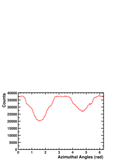
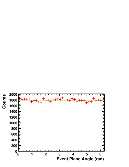
Figure 2: (Color online) On top is a typical azimuthal distribution of particles (pions, third centrality bin) at 40$A$ GeV. On the bottom is the azimuthal distribution of the first harmonic event planes after correction for the laboratory azimuthal anisotropies.

In the standard method, event plane determinations from such a distribution would obviously lead to acceptance biased event planes. As long as each bin in the acceptance is populated significantly, the bias can be removed as described below by recentering the particles in the plane perpendicular to the beam for each rapidity and $p_{t}$ bin, in such a way that the event plane distribution becomes flat. The result of this procedure is exemplified for the first harmonic in Fig. 2 bottom.

In the cumulant method, the main contributions of the detector inefficiency, that is, spurious correlations which have nothing to do with physical (flow or nonflow) correlations, are automatically removed. The only required acceptance corrections amount to a global multiplicative factor which depends solely on the specific detector under study, and can thus be calculated separately from the flow analysis Borghini:2001vi . Further details will be given in Sec. IV.2.

IV Methods

In this section, we recall the principles of the standard (Sec. IV.1) and cumulant (Sec. IV.2) methods of flow analysis.

IV.1 Standard method

The standard method Ollitrault:1997di ; Poskanzer:1998yz correlates the azimuthal angles of particles, $\phi$, with an estimated event plane to obtain the observed coefficients in a Fourier expansion in the plane transverse to the beam. The observed coefficients are then divided by the resolution of the event plane obtained from the correlation of the estimated event planes of two random subevents. The estimated event plane angle, $\Phi_{n}$, are obtained from the azimuthal angles of the $Q_{n}$ vectors whose $x$ and $y$ components are defined by:

$$Q_{n}\cos n\Phi_{n} = \sum_{i}w_{i}\left(\cos n\phi_{i}-\left\langle\cos n\phi\right\rangle\right),$$

$$Q_{n}\sin n\Phi_{n} = \sum_{i}w_{i}\left(\sin n\phi_{i}-\left\langle\sin n\phi\right\rangle\right)\,,$$ (2)

where $n$ is the harmonic order and the sum is taken over the $M$ particles in the event. In this work the weights, $w_{i}$, have been taken to be $p_{t}$ for the second harmonic and $y$ in the center of mass for the first harmonic. To make the event plane isotropic in the laboratory in order to avoid acceptance correlations, we have used the recentering method Poskanzer:1998yz . The mean $\left\langle\sin n\phi\right\rangle$ and $\left\langle\cos n\phi\right\rangle$ values in the above equation were calculated as a function of $p_{t}$ and $y$ for all particles in all events in a first pass through the data, and then used in a second pass to recenter the $Q_{n}$ vector to be isotropic as shown in Fig. 2 bottom. The mean sin and cos values were stored in a matrix of 20 $p_{t}$ values and 50 $y$ values for each harmonic. Particles were only used for the event plane determination if the absolute value of the mean sin and cos values for that bin were less than 0.2. Then the flow values are calculated by

$$v_{n}=\frac{\left\langle\cos(n(\phi_{i}-\Phi_{n}))\right\rangle}{\left\langle\cos(n(\Phi_{n}-\Phi_{RP}))\right\rangle}.$$ (3)

If particle $i$ was used also for the event plane determination, its contribution to $Q_{n}$ is subtracted before calculating $\Phi_{n}$, so as to avoid autocorrelations. The denominator is called the resolution and corrects for the difference between the estimated event plane and the real reaction plane, $\Phi_{RP}$. It is obtained from the resolution of the subevent event planes, which is $\sqrt{\left\langle\cos(n(\Phi_{a}-\Phi_{b}))\right\rangle}$. The resolution of the full event plane, for small resolution, is approximately $\sqrt{2}$ larger, but the actual equation in Ref. Poskanzer:1998yz was used for this calculation. It was found to be more accurate to calculate $v_{2}$ relative to the second harmonic event plane, $\Phi_{2}$, although the sign of $v_{2}$ was determined to be positive by correlation with the first harmonic event plane $\Phi_{1}$. The sign of $v_{1}$ was set so that protons at high rapidity have positive $v_{1}$ as described below. The software used in this analysis was derived from that used for the STAR experiment Ackermann:2000tr .

Equation (3) is the most general form to determine $v_{n}$. In the case of the NA49 experiment the main losses are concentrated around 90 deg and 270 deg in the up and down directions. (See Fig. 2 top.) In order to limit the analysis to the regions of more uniform acceptance a cut on the particle azimuthal angle was applied: Particles with $\cos(2\phi)<0$ are cut out. This however requires large acceptance corrections if Eq. 3 is used for $v_{2}$ determination. The correlation term may be modified in Eq. (3) in order to select azimuthal regions with small distortions. Its numerator may be rewritten in the form of a sum of products instead of a difference of angles:

$$\left\langle\cos(n\phi_{i})\cdot\cos(n\Phi_{n})\right\rangle+\left\langle\sin(n\phi_{i})\cdot\sin(n\Phi_{n})\right\rangle.$$ (4)

Since the (ideal) inclusive azimuthal distributions in A+A collisions are flat by definition, both terms must be of equal magnitude and $v_{n}$ can be calculated by 2 times either the first or second term. The cut applied on the azimuthal angle ($\cos(2\phi)<0$) leads to large corrections to the cosine term in Eq. (4). Therefore, for the second harmonic at 40$A$ GeV the numerator in the $v_{2}$ calculation was done using the expression

$$2\left\langle\sin(n\phi_{i})\cdot\sin(n\Phi_{n})\right\rangle.$$ (5)

The same line of argument applies to the denominator of Eq. (3) where again only the sin terms were used and the subevent plane resolution was increased by a factor of $\sqrt{2}$:

$$v_{n}=\frac{2\cdot\left\langle\sin(n\phi_{i})\cdot\sin(n\Phi_{n})\right\rangle}{\sqrt{2}\cdot\left\langle\sin(n\Phi_{n})\cdot\sin(n\Phi_{RP})\right\rangle}$$ (6)

Determination of $v_{2}$ by Eq. 6 requires the acceptance correction only for losses in the selected angular ranges.

A momentum conservation correction for the first harmonic was made as described in Ref. Borghini:2002mv . The correction is made to the observed differential flow values before they are divided by the event plane resolution. Figure 3 shows that this correction, without any adjustable parameter, makes the directed flow curve cross zero at midrapidity. The figure also shows that because this correction is proportional to $p_{t}$ there is a large effect at high $p_{t}$. There is no effect on the elliptic flow because it is calculated relative to the second harmonic event plane. Table 2 shows the parameters used in making this correction.

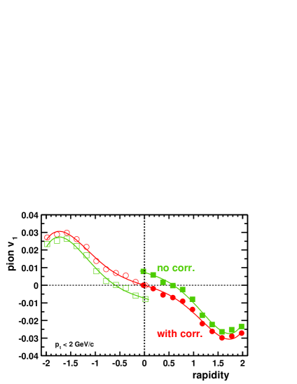
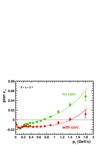
Figure 3: (Color online) Charged pion directed flow as a function of rapidity (top) and $p_{t}$ (bottom) for minimum bias 158$A$ GeV Pb + Pb. Shown are $v_{1}$ before (squares) and after (circles) correction for momentum conservation. The open points in the top graph have been reflected about midrapidity. The solid lines are polynomial fits.

Table 2: Listed for the two beam energies and six centralities are: $N$, the estimated total multiplicity of charged plus neutral hadrons over all phase space; $\left\langle p_{t}^{2}\right\rangle$, the estimated mean $p_{t}^{2}$ of all hadrons over all phase space; $M$, the mean multiplicity of particles used for the event plane determination; $f$, the fraction defined by Eq. (17) in Ref. Borghini:2002mv , which controls the correction for momentum conservation; $\chi_{1}$, the first harmonic resolution parameter for the full event plane (it follows the convention of Ref. Ollitrault:ba and is $\sqrt{2}$ smaller than defined in Ref. Poskanzer:1998yz ); the resolution of the first harmonic full event plane; the percent increase in the resolution due to momentum conservation, and the resolution of the second harmonic event plane. The first two centralities at 158$A$ GeV had more restrictive $p_{t}$ cuts. The first centrality bin at 40$A$ GeV did not have sufficient statistics to determine the second harmonic event plane.

Centrality	1	2	3	4	5	6
158$A$ GeV
$N$	2402	1971	1471	1028	717	457
$\left\langle p_{t}^{2}\right\rangle$ (GeV${}^{2}/c^{2}$)	0.32	0.32	0.31	0.30	0.28	0.27
$M$	119	181	154	110	78	46
$f$	0.07	0.14	0.17	0.17	0.18	0.17
$\chi_{1}$	0.25	0.27	0.40	0.44	0.48	0.47
resolution 1st	0.22	0.24	0.34	0.38	0.40	0.40
res. increase, %	4	16	11	9	7	7
resolution 2nd	0.23	0.28	0.36	0.40	0.37	0.29
40$A$ GeV
$N$	1473	1215	913	643	453	290
$\left\langle p_{t}^{2}\right\rangle$ (GeV${}^{2}/c^{2}$)	0.39	0.38	0.38	0.36	0.34	0.32
$M$	89.3	76.4	59.5	42.2	29.7	17.2
$f$	0.11	0.11	0.11	0.12	0.12	0.11
$\chi_{1}$	0.23	0.23	0.30	0.34	0.38	0.40
resolution 1st	0.20	0.20	0.26	0.29	0.33	0.34
res. increase, %	14	16	8	6	5	4
resolution 2nd	-	0.13	0.25	0.31	0.25	0.21

IV.2 Cumulant method

In this section we first recall the motivations for developing alternative methods of flow analysis. We then explain the principle of the method. Unlike the standard method, the cumulant method yields in principle several independent estimates of directed and elliptic flow, which will be defined below. Finally, we describe the practical implementation of the method.

At the core of the standard method outlined in Sec. IV.1 lies a study of two-particle correlations: one correlates either two subevents, to derive the event plane resolution, or one particle with (a second particle belonging to) the $Q_{n}$ vector. The basic assumption is that the correlation between two arbitrary particles is mainly due to the correlation of each single particle with the reaction plane, that is, due to flow. However, there exist other sources of two-body correlations, that do not depend on the reaction plane; for instance, physical correlations arising from quantum (HBT) effects, global momentum conservation, resonance decays, or jets. At SPS energies, it turns out that these “nonflow” two-particle correlations are a priori of the same magnitude as the correlations due to flow Dinh:1999mn ; Borghini:2000cm , at least in some phase space regions. While some of these correlations can be taken into account in the standard method with a minimal modeling of the collisions (see end of Sec. IV.1), others cannot be estimated as reliably.

This observation motivated the elaboration of new methods of flow analysis, which are much less biased by nonflow correlations than the standard method Borghini:2000sa . The basic idea of the methods is to extract flow from multiparticle azimuthal correlations, instead of using the correlation between two particles only. Naturally, the measured $k$-body correlations also consist of contributions due to flow and to nonflow effects. Nevertheless, by performing a cumulant expansion of the measured correlations, it is possible to disentangle the flow contribution from the other, unwanted sources of correlations. Thus, at the level of four-particle correlations, one can remove all nonflow two- and three-particle correlations, keeping only the correlation due to flow, plus a systematic uncertainty arising from genuine nonflow four-particle correlations, which is expected to be small.

The cumulant method not only minimizes the influence of nonflow correlations; it also provides several independent estimates of $v_{1}$ and $v_{2}$, which will be labeled by the order $k$ at which the cumulant expansion is performed: for instance, $v_{2}\{4\}$ denotes our estimate of $v_{2}$ using cumulants of $4$-particle correlations, etc. Generally speaking, the systematic error due to nonflow correlations decreases as the order $k$ increases, at the expense of an increased statistical error.

To be more specific, we first consider a simplified situation where one wishes to measure the average value of the flow $v_{n}$ over the detector acceptance, which is assumed to have perfect azimuthal symmetry. The lowest order estimate of $v_{n}$ from two-particle correlations, $v_{n}\{2\}$, is then defined by

$$v_{n}\{2\}^{2}\equiv\left\langle e^{in(\phi_{1}-\phi_{2})}\right\rangle$$ (7)

where brackets denote an average value over pairs of particles emitted in a collision, and over events. Please note that $v_{n}\{2\}$ is a priori consistent with the value given by the standard method, Eq. (3), at least if the cuts in phase space are identical in both analyses.

Higher order estimates are obtained from two complementary multiparticle methods. The first one Borghini:2001vi measures the flow harmonics separately, either $v_{1}$ or $v_{2}$. For instance, the four-particle estimate $v_{n}\{4\}$ is defined by

$$-v_{n}\{4\}^{4} \equiv \left\langle e^{in(\phi_{1}+\phi_{2}-\phi_{3}-\phi_{4})}\right\rangle$$ (10)

$$-\left\langle e^{in(\phi_{1}-\phi_{3})}\right\rangle\left\langle e^{in(\phi_{2}-\phi_{4})}\right\rangle$$

$$-\left\langle e^{in(\phi_{1}-\phi_{4})}\right\rangle\left\langle e^{in(\phi_{2}-\phi_{3})}\right\rangle,$$

where the average runs over quadruplets of particles emitted in the collision, and over events. The right-hand side defines the cumulant of the four-particle correlations. This can be generalized to an arbitrary even number of particles, which yields higher order estimates $v_{n}\{6\}$, $v_{n}\{8\}$, etc.

The second multiparticle method Borghini:2002vp was used to analyze directed flow $v_{1}$. It relies on a study of three-particle correlations which involve both $v_{1}$ and $v_{2}$:

$$\left\langle e^{i(\phi_{1}+\phi_{2}-2\phi_{3})}\right\rangle\simeq(v_{1})^{2}v_{2}.$$ (11)

In the case of NA49, we shall see that the first multiparticle method provides reliable estimates of $v_{2}$ (the most reliable was found to be $v_{2}\{2\}$ at 40$A$ GeV and $v_{2}\{4\}$ at 158$A$ GeV, as will be discussed later). Then, the above equation can be used to obtain an estimate of $v_{1}$, which is denoted by $v_{1}\{3\}$ since it involves a $3$-particle correlation. As shown in Ref. Borghini:2002vp , and will be seen below in Sec. V.2, $v_{1}\{3\}$ offers the best compromise between statistical errors (which prevent obtaining $v_{1}\{4\}$ with the first method) and systematic errors from nonflow correlations, which plague the lowest order estimate $v_{1}\{2\}$. In particular, among other nonflow correlations, $v_{1}\{3\}$ is insensitive to the correlation due to momentum conservation, so that one need not compute it explicitly as in the case of the standard method. As a matter of fact, a straightforward calculation using the three-particle correlation due to momentum conservation, given by Eq. (12) in Ref. Borghini:2003ur , shows that the contribution of $p_{t}$ conservation to the average $\left\langle e^{i(\phi_{1}+\phi_{2}-2\phi_{3})}\right\rangle$ is $\left\langle p_{t}\right\rangle^{2}/(N^{2}\left\langle p_{t}^{2}\right\rangle)$, roughly smaller than $1/N^{2}$. (Please note that this three-particle correlation is positive, while the two-particle one is negative, back-to-back.) With the values of $N$ listed in Table 2, this ranges from $0.2\times 10^{-6}$ to $4.8\times 10^{-6}$ at 158$A$ GeV: for the various centrality bins, this is a factor of 10 smaller than the $(v_{1})^{2}v_{2}$ values we shall find. Therefore, the contamination of correlations due to transverse momentum conservation in our derivation of the estimate $v_{1}\{3\}$ is indeed negligible.

The flow analysis with either multiparticle method consists of two successive steps. The first step is to estimate the average value of $v_{1}$ and $v_{2}$ over phase space (in practice, these are weighted averages, as we shall see shortly), which we call “integrated flow”. This is done using Eq. (7), Eq. (10) or Eq. (11), which yield $v_{n}\{2\}$, $v_{n}\{4\}$ and $v_{1}\{3\}$, respectively. The second step is to analyze differential flow, $v_{n}(p_{t},y)$, in a narrow $(p_{t},y)$ window. For this purpose, one performs averages as in Eqs. (7-11), where the particle with angle $\phi_{1}$ belongs to the $(p_{t},y)$ window under study, while the average over $\phi_{2}$, $\phi_{3}$, $\phi_{4}$ is taken over all detected particles. The left-hand sides of Eqs. (7,10) and the right-hand side of Eq. (11) are then replaced by $v_{n}\{2\}(p_{t},y)\times v_{n}\{2\}$, $v_{n}\{4\}(p_{t},y)\times v_{n}\{4\}^{3}$, $v_{1}\{3\}(p_{t},y)\times v_{1}\{3\}v_{2}$, respectively. This defines the estimates of differential flow from 2, 4 and 3 particle correlations. Note that they can be obtained only once the integrated flow is known. In order to reduce the computing time, the analysis was performed over 20 $p_{t}$ bins of 0.1 GeV/$c$ and 20 $y$ bins of 0.3 rapidity units (instead of 50 $y$ bins in the standard method).

In the case of NA49, the use of higher order cumulants was limited by statistical errors, in particular for differential flow. In practice, up to four estimates of integrated elliptic flow were obtained, namely $v_{2}\{2\}$, $v_{2}\{4\}$, $v_{2}\{6\}$ and $v_{2}\{8\}$, but at most two ($v_{2}\{2\}$ and $v_{2}\{4\}$) for differential flow. In the case of directed flow, at most three estimates were obtained for integrated flow ($v_{1}\{2\}$, $v_{1}\{3\}$ and $v_{1}\{4\}$) and two for differential flow ($v_{1}\{2\}$ and $v_{1}\{3\}$).

The practical implementation of these multiparticle methods is described in detail in Refs. Borghini:2001vi ; Borghini:2002vp . In order to illustrate the procedure, we recall here how estimates of integrated (directed or elliptic) flow are obtained from the first multiparticle method outlined above. One first defines the generating function

$$\left\langle G_{n}(z)\right\rangle=\left\langle\prod_{j=1}^{M}\left(1+\frac{w_{n}(j)}{M}(z\,e^{-in\phi_{j}}+z^{*}\,e^{in\phi_{j}})\right)\right\rangle,$$ (12)

where $z$ is a complex variable, and $z^{*}$ its complex conjugate. The product runs over particles detected in a single event, and $w_{n}(j)\equiv w_{n}({p_{t}}_{j},y_{j})$ is the weight attributed to the $j$-th particle with azimuthal angle $\phi_{j}$. Angular brackets denote an average over events. A similar generating function for the analysis of directed flow from three-particle correlations can be found in Ref. Borghini:2002vp . Weights in Eq. (12) are identical to the weights used in the standard method (see Eq. (2)), namely $y$ in the center of mass for $v_{1}$, and $p_{t}$ for $v_{2}$. As in the standard method, they are introduced in order to reduce the statistical error.

In Eq. (2), we use the same value of $M$ for all events in a given centrality bin. This value has been fixed to 80% of the average event multiplicity in the bin. The small fraction of events having multiplicity less than $M$ are rejected. For the events having multiplicity greater than $M$, the $M$ particles required to construct the generating function are chosen randomly. Alternatively, one could have chosen for $M$ in Eq. (2) the total event multiplicity. We have checked on a few examples that results are the same within statistical errors. Note that the value of $M$ is much larger for the cumulant method (Table 3) than for the standard method (Table 2). In the standard method, we have seen that cuts were performed in order to minimize the azimuthal asymmetry of the detector, resulting in a lower value of $M$. In the cumulant method, such detector effects are taken into account, as will be explained below, so that cuts are not necessary. Furthermore, statistical errors are extremely sensitive to $M$ for higher-order estimates, so that it is important to use as many particles as possible.

The cumulants of $2k$-particle correlations, $c_{n}\{2k\}$ are then obtained by expanding in power series the generating function of cumulants, ${\cal C}_{n}(z)$, defined as

$${\cal C}_{n}(z) = M\left(\left\langle G_{n}(z)\right\rangle^{1/M}-1\right)$$ (13)

$$\equiv \sum_{k=0}^{+\infty}c_{n}\{2k\}\left\langle w_{n}^{2}\right\rangle^{k}\frac{|z|^{2k}}{(k!)^{2}}.$$ (14)

The average value of the weight squared, $\left\langle w_{n}^{2}\right\rangle$, has been introduced so that the cumulants $c_{n}\{2k\}$ are dimensionless. In practice, the cumulants are obtained from the generating function using interpolation formulas given in Appendix A. Finally, each cumulant yields an independent estimate of the integrated flow $v_{n}$:

$$c_{n}\{2\}=v_{n}\{2\}^{2} c_{n}\{4\}=-v_{n}\{4\}^{4}\,,$$ , (15)

$$c_{n}\{6\}=4\,v_{n}\{6\}^{6} c_{n}\{8\}=-33\,v_{n}\{8\}^{8}\ldots$$ , (16)

A similar procedure holds for differential flow. If the cumulant extracted from the data comes out with the wrong sign (for instance, a positive number for $c_{n}\{4\}$), one cannot obtain the corresponding flow estimate ($v_{n}\{4\}$). As we shall see in Sec. V, this does occur, most often for central collisions where the flow is small. There are two reasons for this: statistical fluctuations, which may be large for multiparticle cumulants Borghini:2001vi ; nonflow correlations, in particular for two-particle cumulants, which may be opposite to the correlations due to flow (see the effect of momentum conservation on directed flow in Sec.V.2).

In the last equation, $v_{n}$ denotes the weighted integrated flow, defined as

$$v_{n}\equiv\frac{\langle w_{n}e^{in(\phi-\Phi_{R})}\rangle}{\sqrt{\langle w_{n}^{2}\rangle}}.$$ (17)

It is dimensionless, as it should be. We decided to normalize with $\sqrt{\langle w_{n}^{2}\rangle}$ rather than $\langle w_{n}\rangle$ since the weight $w_{n}$ can be negative: for a perfect detector, $\left\langle w_{1}\right\rangle=\left\langle y\right\rangle$ would vanish! One should note that this integrated flow differs from that obtained in the standard method, which integrates the doubly differential flow without weights. Since the average values in Eq. (17) are taken over the whole detector acceptance, the integrated $v_{n}$ is a strongly detector-dependent quantity, whose absolute value has little physical significance. It is essentially an intermediate step: as explained above, one can analyze differential flow only once integrated flow is known. However, we shall see in Sec. V.4 that the centrality dependence of $v_{n}$ is meaningful. The magnitude of integrated flow also determines the magnitude of statistical errors through the resolution parameter $\chi_{n}=v_{n}\sqrt{M}$, which is essentially the same quantity as for the standard method. Using weights increases $\chi_{n}$ roughly by a factor of 1.2. In Table 3 are presented the multiplicity used in the cumulant method and the corresponding $\chi$ parameters.

Table 3: Listed for the two beam energies and six centralities are: $M$, multiplicity used in the cumulant method, Eq.  (12), for the reconstruction of the integrated flow; $\chi_{n}=v_{n}\sqrt{M}$, the resolution parameter, where $v_{n}$ is a (rescaled) weighted flow, see Eq. (17). The multiplicities are larger for the cumulant method than for the standard method because all particles were used, including particles in the backward hemisphere.

Centrality	1	2	3	4	5	6
158$A$ GeV
$M$	591	528	419	301	209	109
$\chi_{1}$	-	0.27	0.33	0.39	0.41	0.35
$\chi_{2}$	0.27	0.42	0.63	0.67	0.62	0.44
40$A$ GeV
$M$	318	257	185	120	80	42
$\chi_{1}$	-	0.003	0.19	0.23	0.16	0.26
$\chi_{2}$	-	0.45	0.43	0.42	0.40	0.23

Although the formalism may at first sight look complicated, its various features make it the simplest to use in practice, for several reasons. First, the several estimates are obtained from a single generating function. Second, the generating function automatically involves all possible $k$-tuplets of particles in the construction of the $k$-particle cumulants. Last but not least, the formalism can be used even if the detector does not have perfect azimuthal symmetry. In this case, Eqs. (7-11) no longer hold. Other terms must be added in order to remove the spurious, nonphysical correlations arising from detector inefficiencies, and the number of these terms increases tremendously as the order of the cumulant increases. With the generating-function formalism, they are automatically included and require no additional work.

When the azimuthal coverage of the detector is strongly asymmetric, further acceptance corrections must be made, which amount to a global multiplicative factor  in the relations Eqs. (15) between the cumulants $c_{n}\{k\}$ and the flow estimates $v_{n}\{k\}$ Borghini:2001vi ; Borghini:2002vp . In the case of the NA49 acceptance, the corrections are negligible at 158$A$ GeV but can become significant at 40$A$ GeV. We present the range of the corrections factors on the reconstructed flow values in Table 4.

Table 4: Acceptance correction factors on the reconstructed values of the flow $v_{n}\{k\}$. For integrated flow, the range corresponds to the various centrality bins. For differential flow, the correction factors are calculated in centrality bin 4 and the range corresponds to the various ($p_{t},y$) bins. The larger corrections are for the highest $p_{t}$ or $y$ values.

158$A$ GeV	$v_{1}\{2\}$	$v_{1}\{3\}$	$v_{2}\{2\}$	$v_{2}\{4\}$	40$A$ GeV	$v_{1}\{2\}$	$v_{1}\{3\}$	$v_{2}\{2\}$	$v_{2}\{4\}$
Integrated	1.00	1.01	1.00	1.00	Integrated	1.03 – 1.04	1.07 – 1.09	1.03 – 1.04	1.01
Differential	1.00 – 1.08	1.01	1.00 – 1.02	1.01 – 1.06	Differential	1.07 – 1.23	1.10 – 1.17	1.07 – 1.29	1.01 – 1.78

IV.3 Systematic uncertainties

Various measures are introduced above in order to quantify azimuthal correlations of particles produced in heavy ion collisions. These measures are used in the data analysis with the aim to extract information on directed and elliptic flow of primary charged pions and protons emitted in the interaction of two nuclei. The measured correlations consist, however, not only of the genuine flow correlations, but also from other physical correlations of primary hadrons (nonflow physical correlations) as well as correlations introduced by the imperfectness of the measuring methods. The issue of nonflow physical correlations is addressed in the description of the methods in Secs. IV.1,  IV.2 and, in particular, in Sec. V.5. In the following we discuss various sources of detector induced correlations, as well as corrections and cuts used to reduce their influence on the results and the systematic uncertainties.

The geometrical acceptance of the detector is not uniform in azimuthal angle as seen in Fig. 2 top. This effect is corrected for in both methods. As the geometrical acceptance of the detector can be probed to high accuracy by the particle yields, the systematic uncertainty caused by non-uniform acceptance is small except as noted below. The majority of the events selected by the hardware trigger and off–line event cuts (see Sec. III.2) are Pb+Pb collisions. However, there is a small ($<5\%$) contamination in low multiplicity events from collisions of the Pb beam with the material surrounding the target foil. A possible bias caused by this contamination was estimated by varying off–line selection cuts on the primary vertex position. No influence on the magnitude of the $v_{1}$ and $v_{2}$ was observed.

About 90% of tracks selected by the track selection cuts (see Sec. III.2) are tracks of primary hadrons coming from the main interaction vertex. The remaining fraction of tracks originates predominately from weak decays and secondary interactions occurring in the detector material. In order to estimate a possible bias due to this contamination the cuts on track distance from the reconstructed event vertex ($b_{x}$,$b_{y}$) were varied as shown in Fig. 4 with little effect on the results.

Figure 4: (Color online) Rapidity dependence of pion elliptic flow for different cuts on the track impact parameter. The sets of the cuts were chosen to be 1.0 cm for $b_{x}$ and 0.2 cm for $b_{y}$ for the tight cut. For the open case no cut was used. The standard cut is 3.0 cm for $b_{x}$ and 0.5 cm for $b_{y}$.

The efficiency of track reconstruction and track selection cuts depends on track density in the detector and this efficiency is the lowest ($\approx 80\%$) for central Pb+Pb collisions at 158$A$ GeV at midrapidity. The systematic uncertainty due to track losses was estimated by varying track selection cuts (see Sec. III.2). Additionally, data taken at the two magnetic field polarities and during two running periods were analyzed separately and the results compared in Fig. 5. The systematic variations are largest in near central collisions for $v_{1}$ ($\Delta v_{1}=0.005$ ) and in peripheral collisions for $v_{2}$ ($\Delta v_{2}=0.01$).

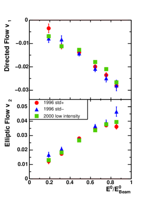
Figure 5: (Color online) Centrality dependence of results for different data sets taken with the same beam energy, same centrality definition, but two different field polarities and beam intensities. The most recent data set was taken after some changes to the detector and analysis procedures.

The influence of the particle identification procedures on the flow values was probed by changing the energy loss criteria within reasonable limits. The resulting variation of $v_{1}$ and $v_{2}$ are below 0.005. The integrations over $p_{t}$ and rapidity involve a weighting procedure on the basis of differential cross sections (see Sec V). These cross sections are available at 40$A$ GeV only for pions in central collisions, for other cases they were estimated based on data systematics. Variation of the cross section weights within reasonable limits results in variations below 0.001 for $v_{2}$ and 0.005 for $v_{1}$.

The azimuthal coverage of the NA49 TPCs is significantly reduced at 40$A$ GeV as compared to 158$A$ GeV (see Sec. III.3). Modifications to the standard analysis method were necessary to reduce the systematic errors. The validity of the results from the modified method were scrutinized by applying it to the 158$A$ GeV data. The results of this test are stable and in agreement with those of the standard method for mid-central collisions. In near central and peripheral collisions large relative differences are taken as estimate of systematic uncertainties. These are significant, if low event multiplicity or low flow values make the event plane determination unreliable.

The results of our study of systematic uncertainties can be summarized as follows. The systematic error of $v_{2}(p_{t},y)$ and $v_{1}(p_{t},y)$ for pions in mid-central and peripheral collisions is 0.005 and 0.002 respectively. For central collisions the numbers increase to 0.01 for both. The error for protons for mid-central and peripheral collisions is 0.005 for $v_{2}$ and 0.01 for $v_{1}$. For central collisions it increases to about 0.03 for both. At 40$A$ GeV these errors could be 50% larger than those at 158$A$ GeV. Note that the errors plotted in all figures are statistical ones only.

V Results

Both methods outlined in Sec. IV have been applied at 40$A$ GeV and 158$A$ GeV. The double differential flow values $v_{n}(p_{t},y)$ for each harmonic as obtained from the methods were tabulated as a function of $p_{t}$, $y$, and centrality. Integration of $v_{n}(p_{t},y)$ to obtain $v_{n}(p_{t})$ or $v_{n}(y)$ values was done by averaging over the integration variable using the cross sections of the particles as weights. The cross section values at 158$A$ GeV had been parametrized crosssections and were available as a macro. Since no cross sections were available at 40$A$ GeV for non-central collisions, the width of the pion Gaussian rapidity distribution and the separation of the two proton rapidity Gaussian distributions were scaled down by the ratio of the beam rapidities at 40 and 158$A$ GeV. Since we chose larger $y$ bins in the cumulant method than in the standard method, the integration over rapidity was not performed over exactly the same $y$ range. More precisely, the upper limit is always smaller for the cumulant method because the results for proton flow did not seem to be very stable with respect to integration up to high rapidity values. In the cumulant $v(p_{t})$ graphs the indicated $y$ ranges refer to the cumulant results; the reproduced standard method results in these graphs have the $y$ ranges indicated in the preceding standard method plots. The results are presented for three centrality bins (two successive bins have been combined, weighted with the known cross sections and the fraction of events in each bin, see Table 1) and also integrated over the first five centrality bins (weighted with the known cross sections and the fraction of the geometric cross section for each bin given in Table 1), which we call minimum bias. We present elliptic flow (Sec. V.1), directed flow (Sec. V.2), minimum bias results (Sec. V.3), centrality dependence (Sec. V.4), nonflow effects (Sec. V.5), and beam energy dependence (Sec. V.6). The standard method $v_{1}$ values have been corrected for momentum conservation but the cumulant method $v_{1}\{2\}$ values have not.

In the graphs of flow as a function of rapidity the points have been reflected about midrapidity and fitted with polynomial curves to guide the eye. Please note that we always use the rapidity in the center of mass, and to calculate this the nominal laboratory rapidity of the center of mass was taken to be 2.92 at 158$A$ GeV and 2.24 at 40$A$ GeV. In the graphs of flow as a function of $p_{t}$ the smooth curves shown to guide the eye were obtained by fitting to a simple hydrodynamic motivated Blast Wave model as described in Ref. Snellings:2001 ; pasi2 but generalized to also describe $v_{1}$:

$$v_{n}(p_{t})=\frac{\int_{0}^{2\pi}d\phi_{b}\cos(n\phi_{b})I_{n}(\alpha_{t})K_{1}(\beta_{t})(1+2s_{n}\cos(n\phi_{b}))}{\int_{0}^{2\pi}d\phi_{b}I_{0}(\alpha_{t})K_{1}(\beta_{t})(1+2s_{n}\cos(n\phi_{b}))},$$ (18)

where the harmonic $n$ can be either one or two, where $I_{0}$, $I_{n}$, and $K_{1}$ are modified Bessel functions, and where $\alpha_{t}(\phi_{b})=(p_{t}/T_{f})\sinh(\rho(\phi_{b}))$ and $\beta_{t}(\phi_{b})=(m_{t}/T_{f})\cosh(\rho(\phi_{b}))$. The basic assumptions of this model are boost-invariant longitudinal expansion and freeze-out at constant temperature $T_{f}$ on a thin shell, which expands with a transverse rapidity exhibiting a first or second harmonic azimuthal modulation given by $\rho(\phi_{b})=\rho_{0}+\rho_{a}\cos(n\phi_{b})$. In this equation, $\phi_{b}=\phi-\Phi_{RP}$ is the azimuthal angle (measured with respect to the reaction plane) of the boost of the source element on the freeze-out hyper-surface pasi2 , and $\rho_{0}$ and $\rho_{a}$ are the mean transverse expansion rapidity [$v_{0}=\tanh(\rho_{0})$] and the amplitude of its azimuthal variation, respectively. The parameters in this model are $T_{f}$, the temperature, $\rho_{0}$, the transverse flow rapidity, $\rho_{a}$, the azimuthal flow rapidity, and $s$, the surface emission parameter. The $T_{f}$ parameter was fixed and the $s$ parameter was allowed to be non-zero only for pions at 158$A$ GeV. The values of the fit parameters themselves are not very meaningful because the flow values derived from two-particle correlations contain nonflow effects and the values from many-particle analyses have poor statistics, but the fits do provide the curves to guide the eye shown in the $p_{t}$ graphs. The data are clearly not boost invariant, but since we use the blast wave model only to fit the $p_{t}$ dependence of the flow, it was felt that a more sophisticated model was not warranted. When the fits would not converge the points were just connected, giving rise to the jagged lines in some graphs.

The error bars shown for the standard method are the standard deviation of the data. For the cumulant method, they are calculated analytically following the formulas given in Refs. Borghini:2001vi ; Borghini:2002vp . Tables of the data can be found on the web at http://na49info.cern.ch/na49/Archives/Data/FlowWebPage/.

V.1 Elliptic flow

V.1.1 158$A$ GeV

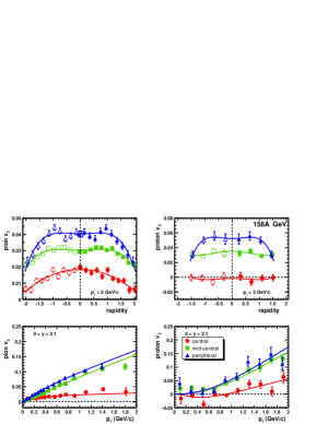
Figure 6: (Color online) Elliptic flow obtained from the standard method as a function of rapidity (top) and transverse momentum (bottom) for charged pions (left) and protons (right) from 158$A$ GeV Pb + Pb. Three centrality bins are shown. The open points in the top graphs have been reflected about midrapidity. Solid lines are polynomial fits (top) and Blast Wave model fits (bottom).

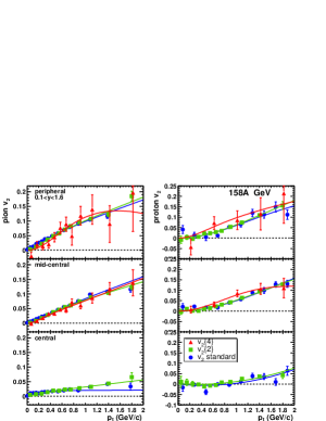
Figure 7: (Color online) Elliptic flow of charged pions (left) and protons (right) from the cumulant method as a function of transverse momentum in 158$A$ GeV Pb + Pb collisions. Three centrality bins are shown with results from the standard method, from cumulants for two-particle correlations ($v_{2}\{2\}$), and from cumulants for four-particle correlations ($v_{2}\{4\}$). Solid lines are from Blast Wave model fits.

Figure 8: (Color online) Same as Fig. 7, as a function of rapidity. The open points have been reflected about midrapidity. Solid lines are from polynomial fits. Please note the different vertical scales.

Results from 158$A$ GeV collisions are displayed in Fig. 6 (from the standard method) and are compared to the results from the cumulant method in Figs. 7 and 8.

We first discuss results for mid-central collisions (Figs. 7 and 8, middle) for the following reason: as usual in flow analyses, they have smaller errors than peripheral collisions (Figs. 7 and 8, top) due to the larger multiplicity, and also smaller than central collisions (Figs. 7 and 8, bottom) due to the larger value of the flow. By errors, we mean both the statistical error, shown in the figures, and the uncertainty of the contribution of nonflow correlations, which is not known and not shown in the figures. For mid-central collisions, $v_{2}$ is positive over all phase space for pions and protons. As a function of $p_{t}$, it rises linearly for pions up to 2 GeV/c (Fig. 7 middle left). For protons (Fig. 7 middle right), the rise is slower at low $p_{t}$ (quadratic rather than linear up to 1 GeV/c), but interestingly, $v_{2}$ reaches the same value as for pions at 2 GeV/c. All three methods give compatible results within statistical error bars. As a function of rapidity, the pion $v_{2}$ exhibits the usual bell shape (Fig. 8 middle left), with a maximum at mid-rapidity. This maximum, however, is not very pronounced, and $v_{2}$ remains essentially of the same magnitude, between 2% and 3%, over four units of rapidities. For protons (Fig. 8 middle right), the rapidity dependence is similar. Note that $v_{2}(y)$ is slightly larger than for pions, although $v_{2}(p_{t})$ was smaller. This can be explained simply: $v_{2}(y)$ is integrated over $p_{t}$, protons have higher average $p_{t}$ than pions, and $v_{2}$ increases with $p_{t}$. For protons, a small discrepancy appears around $y=0$ between the estimate from the two-particle cumulants ($v_{2}\{2\}$) and the standard reaction plane estimate, which we do not understand, and consider part of our systematic error.

For peripheral collisions, $v_{2}$ is somewhat larger than for mid-central collisions at low $p_{t}$ (Fig. 6 bottom), but comparable at high $p_{t}$. $v_{2}(y)$ is dominated by the low $p_{t}$ region where the yield is larger, hence it is also larger for peripheral than for mid-central collisions (Fig. 6 top). A small discrepancy can be seen around $y=1$ for pions between $v_{2}\{2\}$ and the standard $v_{2}$ (Fig. 8 top left).

For central collisions, elliptic flow is much smaller (Fig. 6). As a consequence, four-particle cumulants could not be used, due to large statistical fluctuations. Contrary to more peripheral collisions, $v_{2}(y)$ is larger for pions than for protons (Figs. 6, top, and 8, bottom), for which it is consistent with zero in the available rapidity range.

We have also compared these results with those of the earlier analysis published in Ref. NA49PRL and updated on the collaboration web page NA49Web . Note that the previous analysis used narrower cuts in $p_{t}$ and $y$, and had much larger statistical errors. Results are compatible for protons, but not for pions. In particular $v_{2}(p_{t})$ is significantly different at low $p_{t}$, where the increase is now much smoother. The earlier analysis was biased by Bose-Einstein correlations Dinh:1999mn , whose contribution is reduced in the present analysis thanks to the $w_{i}=p_{t}$ weights used in Eq. (2), rather than the unit weights used in the previous analysis.

V.1.2 40$A$ GeV

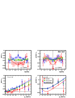
Figure 9: (Color online) Elliptic flow obtained from the standard method as a function of rapidity (top) and transverse momentum (bottom) for charged pions (left) and protons (right) from 40$A$ GeV Pb + Pb. Three centrality bins are shown (“central” corresponds to centrality bin 2 only, see Table 1). The open points in the top graphs have been reflected about midrapidity. Solid lines are polynomial fits (top) and Blast Wave model fits (bottom).

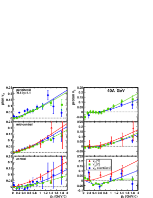
Figure 10: (Color online) Elliptic flow of charged pions (left) and protons (right) obtained from the cumulant method as a function of transverse momentum from 40$A$ GeV Pb + Pb. Three centrality bins are shown. Here, “central” (bottom) corresponds only to centrality bin 2 (see Table 1). Results are shown from the standard method, from cumulants for two-particle correlations ($v_{2}\{2\}$), and from cumulants for four-particle correlations ($v_{2}\{4\}$). The smooth solid lines are from Blast Wave model fits.

Figure 11: (Color online) Same as Fig. 10, as a function of rapidity. The open points have been reflected about midrapidity. Solid lines are from polynomial fits.

Results from 40$A$ GeV collisions are displayed in Figs. 9 (from the standard method), 10, and 11 (from the cumulant method). Both the values of $v_{2}$ and the multiplicities are smaller than at 158$A$ GeV, which results in larger errors.

In mid-central collisions, $v_{2}(p_{t})$ (Fig. 10 middle) is roughly the same as at 158$A$ GeV (Fig. 7 middle), both in shape and magnitude, and all three methods give consistent results. The value of $v_{2}$ at a fixed $p_{t}$ is in fact very similar up to the highest RHIC energy, as pointed out by Snellings Snellings:2003mh . Since the average $p_{t}$ is smaller at 40$A$ GeV than at 158$A$ GeV, however, the corresponding $v_{2}(y)$ is smaller (Fig. 11 middle). As a function of rapidity, both the standard $v_{2}$ and $v_{2}\{2\}$ of pions are remarkably flat. On the other hand, $v_{2}\{4\}$ is bell-shaped, as at 158$A$ GeV, but statistical error bars prevent any definite conclusion. For protons (Fig. 11 middle right), a discrepancy appears between $v_{2}\{2\}$, which is bell-shaped, and the standard $v_{2}$, which has a dip at mid-rapidity.

For peripheral collisions, $v_{2}$ is slightly larger, but similar to mid-central collisions (Fig. 9). The four-particle cumulant result $v_{2}\{4\}$ could not be obtained due to large statistical errors.

At this energy, statistics did not allow the determination of the second harmonic event plane, nor the derivation of estimates from two- or four-particle cumulants for the most central bin. Thus, the “central” bin corresponds to bin 2 only in Figs. 9 to 11. A striking discrepancy appears between the two-particle estimates (standard $v_{2}$ and $v_{2}\{2\}$) and the four-particle cumulant result $v_{2}\{4\}$ in the $p_{t}$ dependence (Fig. 10 bottom). It is closely related to that observed in the rapidity dependence: For pions (Fig. 11, bottom left), the standard $v_{2}$ and $v_{2}\{2\}$ both seem to show a dip at midrapidity, where they are compatible with zero; for protons (Fig. 11, bottom right), the standard $v_{2}$ and $v_{2}\{2\}$ are even negative at midrapidity. By contrast, the four-particle cumulant result, $v_{2}\{4\}$, is positive for both pions and protons and has the usual bell shape, with a maximum value at midrapidity.

Since the difference between two-particle estimates and $v_{2}\{4\}$ is much beyond statistical error bars, this is a hint that the two-particle estimates for pions are affected by nonflow effects (recall that $v_{2}\{4\}$ is expected to be free from two-particle nonflow effects). This could be due to correlations from $\rho$ decays, since $\rho$ mesons are more concentrated near midrapidity, and produce a negative correlation in the second harmonic Borghini:2000cm , which tends to lower the two-particle $v_{2}$ estimates. This effect, however, cannot explain the difference for protons.

While the four-particle cumulant result $v_{2}\{4\}$ for central collisions looks very reasonable in shape (bell shape in rapidity, regular increase with $p_{t}$ for both pions and protons), its magnitude is unusual: it is as large as for mid-central collisions, while we would have expected a significantly smaller value following the observations at 158$A$ GeV.

V.2 Directed flow

V.2.1 158$A$ GeV

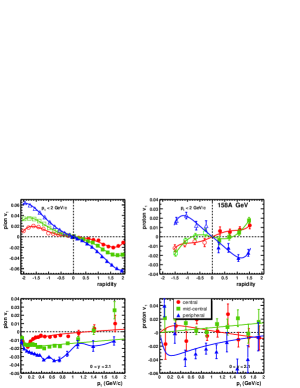
Figure 12: (Color online) Standard directed flow as a function of rapidity (top) and transverse momentum (bottom) for charged pions (left) and protons (right) from 158$A$ GeV Pb + Pb. Three centrality bins are shown. The open points in the top graphs have been reflected about midrapidity. On the top, solid lines are polynomial fits. On the bottom, smooth solid lines are Blast Wave model fits.

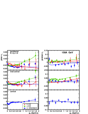
Figure 13: (Color online) Directed flow of charged pions (left) and protons (right) from cumulant method, as a function of transverse momentum in 158$A$ GeV Pb + Pb. Three centrality bins are shown. Here, “central” (bottom) corresponds to centrality bin 2 (see Table 1) only. Results are shown from the standard method, from cumulants for two-particle correlations ($v_{1}\{2\}$), and from cumulants for three-particle correlations ($v_{1}\{3\}$). The $v_{1}\{2\}$ estimates are not corrected for momentum conservation, while the standard method results are. Smooth solid lines are Blast Wave model fits. Please note the different vertical scales.

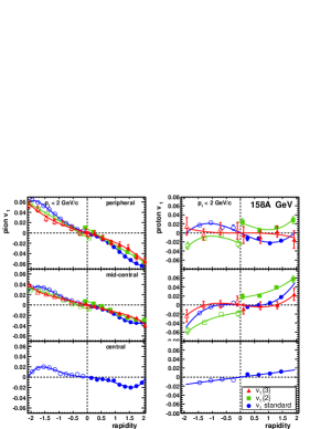
Figure 14: (Color online) Same as Fig. 13, as a function of rapidity. The open points have been reflected about midrapidity. Solid lines are polynomial fits.

Results from collisions at 158$A$ GeV are shown in Figs. 12 (from the standard method),  13, and 14 (from the cumulant method). It can be seen in Fig. 12 top left that the curves for the different centralities all cross zero at midrapidity, indicating that the correction for global momentum conservation in the standard method, shown in Fig. 3 for minimum bias data, also works for the individual centralities. One clearly sees the magnitude of the correction for momentum conservation in Figs. 13, and 14, by comparing the results from the two-particle cumulants, $v_{1}\{2\}$ (squares), which are not corrected, with the results of the standard reaction plane analysis (circles), which are corrected (see Sec. IV.1). The difference between the two results rises linearly with $p_{t}$, and is larger for peripheral collisions (Fig. 13 top) than for mid-central collisions (Fig. 13 middle), as expected from the discussion in Ref. Borghini:2002mv . For central collisions, the negative correlations due to momentum conservation become larger in absolute value than the positive correlations due to flow (because flow is much smaller in central collisions), so that the cumulant $c_{1}\{2\}$ in Eq. (15) becomes negative and the flow estimate $v_{1}\{2\}$ could not be obtained. As a function of rapidity, the difference between $v_{1}\{2\}$ and the standard $v_{1}$ is approximately constant (Fig. 14 top and middle). Unlike the standard $v_{1}$, $v_{1}\{2\}$ does not cross zero at midrapidity, while the true directed flow should. This is a direct indication that $v_{1}\{2\}$ is biased by global momentum conservation (see Fig. 3, top). It is shown merely as an illustration of this effect, and will not be discussed further.

We first discuss the directed flow of pions for mid-central collisions. Its transverse momentum dependence (Fig. 13 middle left) is peculiar. The standard $v_{1}$ (circles) is negative at low $p_{t}$, but then increases and becomes positive above 1.4 GeV/c. The result from the mixed three-particle correlation method [Eq. (11)], $v_{1}\{3\}$, which is expected to be free from all nonflow effects including momentum conservation, is also shown (triangles). Above 0.6 GeV/c, it is compatible with the standard reaction plane estimate, but not with the two-particle estimate $v_{1}\{2\}$. This suggests that nonflow effects are dominated by momentum conservation in this region. Unfortunately, statistical error bars on $v_{1}\{3\}$ are too large at high $p_{t}$ to confirm the change of sign observed in the standard $v_{1}$. Below 0.2 GeV/c, where momentum conservation is negligible, both the standard analysis value and $v_{1}\{2\}$ seem to intercept at a finite value when $p_{t}$ goes to zero. This is suggestive of nonflow effects arising from quantum Bose-Einstein effects between identical pions Dinh:1999mn . The three-particle estimate $v_{1}\{3\}$, which is free of nonflow effects, smoothly vanishes at $p_{t}=0$. This discussion shows that results on directed flow must be interpreted with care, and are more biased by nonflow effects than results on elliptic flow. This is mostly due to the smaller value of directed flow (typically 2% in absolute value, instead of 3% for elliptic flow).

The rapidity dependence of the pion $v_{1}$ for mid-central collisions is displayed in Fig. 14 middle left. One notes that $v_{1}\{3\}$ vanishes at midrapidity (unlike $v_{1}\{2\}$), which confirms that it is automatically corrected for momentum conservation effects. Both $v_{1}\{3\}$ and the standard $v_{1}$ exhibit a smooth, almost linear rapidity dependence. They are in close agreement near mid-rapidity, where we observe clear evidence that the slope is negative. At the more forward rapidities, however, the standard $v_{1}$ becomes larger in absolute value than $v_{1}\{3\}$ and seems to saturate, while the slope becomes steeper for $v_{1}\{3\}$. This small discrepancy can be attributed to the above mentioned Bose-Einstein effects which bias the standard $v_{1}$ at low $p_{t}$. This bias is only present over the phase space used to determine the event plane Dinh:1999mn , i.e. above center-of-mass rapidity $y=1.08$. Note that the value of $v_{1}\{3\}$ is only 4% in absolute value at $y=2$. This is smaller by at least a factor of 5 than the value obtained by the WA98 collaboration in the target fragmentation region (center-of-mass rapidity around -3), where $v_{1}$ reaches 20% for pions Aggarwal:1998vg . There is no overlap between their rapidity coverage and ours, so that we cannot check whether the two analyses are consistent. Nevertheless, this comparison suggests that the slope becomes much steeper toward beam rapidity, a trend already seen on our $v_{1}\{3\}$ result.

In peripheral collisions, the pion $v_{1}$ (Fig. 13 and Fig. 14 top left) has a $p_{t}$ and $y$ dependence very similar to the one in mid-central collisions. Its magnitude, however, is larger, and the increase is more significant than for elliptic flow: $v_{1}\{3\}$ is 50% larger at the most forward rapidities (-6%, instead of -4% for mid-central collisions). In central collisions, $v_{1}\{3\}$ could not be obtained due to large statistical errors. The standard $v_{1}$ (Fig. 13 and Fig. 14 top left) is largest at low $p_{t}$ (below 0.3 GeV/c) and forward rapidities (above $y=1$) where it is biased by Bose-Einstein effects as explained above. This bias is even more important for the centrality bin 1, where a tighter $p_{t}$ cut (below 0.3 GeV/c) was chosen for the event plane determination.

We now discuss the directed flow of protons in mid-central collisions. As a function of $p_{t}$ (Fig. 13 middle right) both the standard $v_{1}$ and $v_{1}\{3\}$ are generally positive but almost consistent with zero. The rapidity dependence (Fig. 14 middle right) is more interesting. $v_{1}$ is flat near midrapidity (error bars are large, but we can safely state that it is flatter than for pions). Only one point, at the most forward rapidity, clearly deviates from zero. This is an essential point, since we use it to resolve the overall sign ambiguity of the $v_{1}$ analysis: at high energies, $v_{1}$ is assumed to be positive for protons at forward rapidities, and this determines the pion flow to be negative in this region (Fig. 14 middle left). In peripheral and central collisions where the sign of the proton $v_{1}$ could not be clearly determined, the pion $v_{1}$ was assumed to be negative for sake of consistency. This sign will be established more firmly at 40$A$ GeV (see below). As already noted for pions, the slope of $v_{1}$ above $y=2$ must be very steep in order to match WA98 results, which give a proton $v_{1}$ of the order of 20% around $y=3$ Aggarwal:1998vg .

In peripheral collisions, there is a discrepancy between the standard $v_{1}$ and $v_{1}\{3\}$ for protons, which is clearly seen on the $p_{t}$ graph (Fig. 13 top right). This difference may be due to nonflow correlations from $\Delta$ decays into protons and pions Borghini:2000cm , which are automatically corrected for in the three-particle analysis, but not in the reaction plane analysis. This contamination from correlations from $\Delta$ decays would then explain why the standard $v_{1}$ has a negative sign at forward rapidities (Fig. 14 top right). In central collisions, where only the reaction plane estimate is available, $v_{1}(p_{t})$ is compatible with zero (Fig. 13 bottom right), but is positive at forward rapidities (Fig. 14 bottom right), as expected.

Let us briefly compare the present results with those of the earlier analysis NA49PRL ; NA49Web . As in the case of elliptic flow, the most significant differences are seen for pions, where $v_{1}$ was biased in the earlier analysis by Bose-Einstein correlations and global momentum conservation Dinh:1999mn ; Borghini:2000cm . The earlier $v_{1}(p_{t})$ is in fact similar to the present $v_{1}\{2\}$ (squares in Fig. 13, middle left), which suffer from the same biases.

V.2.2 40$A$ GeV

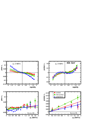
Figure 15: (Color online) Standard directed flow as a function of rapidity (top) and transverse momentum (bottom) for charged pions (left) and protons (right) from 40$A$ GeV Pb + Pb. Three centrality bins are shown. The open points in the top graphs have been reflected about midrapidity. On the top, solid lines are polynomial fits. On the bottom, smooth solid lines are Blast Wave model fits.

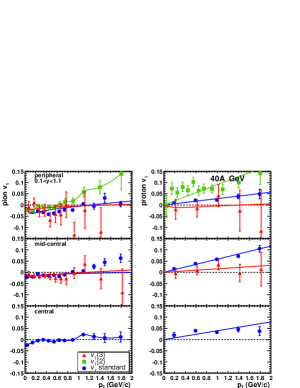
Figure 16: (Color online) Directed flow of charged pions (left) and protons (right) from the cumulant method, as a function of transverse momentum in 40$A$ GeV Pb + Pb. Three centrality bins are shown. Results are shown from the standard method, from cumulants for two-particle correlations ($v_{1}\{2\}$), and from cumulants for three-particle correlations ($v_{1}\{3\}$). Please note that the $v_{1}\{2\}$ estimates are not corrected for momentum conservation, while the standard method results are. Smooth solid lines are Blast Wave model fits.

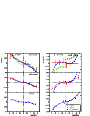
Figure 17: (Color online) Same as Fig. 16, as a function of rapidity. The open points have been reflected about midrapidity. Solid lines are polynomial fits. Please note the different vertical scales.

Results from 40$A$ GeV collisions are shown in Fig. 15 (from the standard method), 16, and 17 (from the cumulant method). In Fig. 15, top, one can see that the standard $v_{1}$ crosses zero at midrapidity for all centralities, which shows that the correlation from global momentum conservation has been properly subtracted. The three-particle results $v_{1}\{3\}$, which is automatically free from all nonflow effects including momentum conservation, also crosses zero at mid-rapidity for peripheral and mid-central collisions (Fig. 17 top and middle). It could not be obtained for central collisions due to large statistical fluctuations. The effect of momentum conservation is even larger than at 158$A$ GeV, as can be seen by comparing $v_{1}\{2\}$ (not corrected) with the standard $v_{1}$ (corrected) for peripheral collisions (Figs. 16 and 17 top). For mid-central and central collisions, the momentum conservation effect is so large that $v_{1}\{2\}$ could not even be obtained, as for central collisions at 158$A$ GeV.

The directed flow of pions (Figs. 15, 16 and 17 left) is similar at 40$A$ GeV and at 158$A$ GeV, both in magnitude and shape. The standard $v_{1}$ and $v_{1}\{3\}$ are compatible. Error bars are larger at the lower energy due to the lower multiplicity, especially for the three-particle result $v_{1}\{3\}$. The nonzero value of the standard $v_{1}$ at low $p_{t}$ (Fig. 15 bottom left) probably results from nonflow Bose-Einstein correlations, as at 158$A$ GeV.

The directed flow of protons, on the other hand, (Figs. 15, 16 and 17 right), is significantly larger at 40$A$ GeV than at 158$A$ GeV. For mid-central collisions, both the standard $v_{1}$ and $v_{1}\{3\}$ clearly differ from zero at forward rapidities (Fig. 17 middle right). As already explained, the proton $v_{1}$ is assumed to be positive at forward rapidities, and this fixes the sign of the pion flow to be negative in this region (Fig. 17 middle left). This is consistent with our prescription at 158$A$ GeV. The standard $v_{1}$ is larger than $v_{1}\{3\}$. The discrepancy is beyond statistical error bars (Fig. 16 middle right) and might be due to some nonflow effect.

Unlike the pion $v_{1}$, the proton $v_{1}$ does not seem to be larger for peripheral collisions than for mid-central collisions. In Figs. 12 and 15, top right panels, the peripheral data seem to exhibit a “wiggle” such that the proton $v_{1}$ has a negative excursion. Due to the large statistical error bars, this can neither be confirmed nor invalidated by the three-particle cumulant results in Figs. 14 and 17, top right. Nevertheless, such a behavior has been predicted Snellings:1999bt due to the variation in stopping in the impact parameter direction in peripheral collisions coupled with the space-momentum correlations of flow Voloshin:QM02 . This is the first experimental observation of this phenomenon.

V.3 Minimum Bias

The results of the standard method integrated over the first five centrality bins weighted with the fraction of the geometric cross section for each bin given in Table 1 are shown in Figs. 18 and 19 for the two beam energies. For 40$A$ GeV $v_{2}$ bin 1 was not included because we had no results for it. (Also, the cumulant data could not be summed for minimum bias graphs because too many centrality bins were missing.) In the lower left graphs, $v_{1}$ for pions shows a sharp negative excursion in the first 100 MeV/$c$ of $p_{t}$. This can also be seen in the graphs for the individual centralities. To describe this feature the Blast Wave fits require a very large $\rho_{0}$ parameter. However, the physical explanation is not clear and the effect may in fact be caused by some very low $p_{t}$ short range nonflow correlation, most probably quantum correlations between pions Dinh:1999mn ; Borghini:2000cm . Similarly, the positive values of $v_{1}$ for pions at high transverse momenta is due to nonflow correlations (see $v_{1}\{3\}$ in Fig. 16). In Fig. 18 lower right, the proton $v_{1}$ is consistent with zero at all $p_{t}$ values because of the accidental cancellation of its positive and negative values at the different centralities.

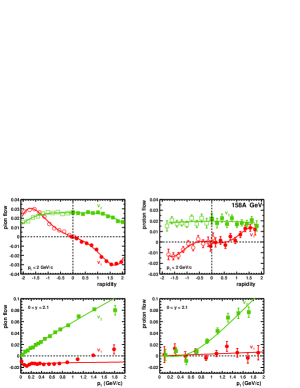
Figure 18: (Color online) Standard minimum bias directed and elliptic flow as a function of rapidity (top) and transverse momentum (bottom) for charged pions (left) and protons (right) from 158$A$ GeV Pb + Pb. Shown are $v_{1}$ (circles) and $v_{2}$ (squares). The open points in the top graphs have been reflected about midrapidity. Solid lines are polynomial fits on the top and Blast Wave model fits on the bottom.

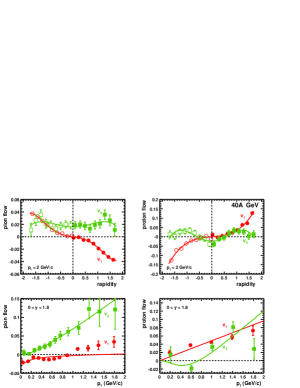
Figure 19: (Color online) Same as Fig.18 for 40$A$ GeV Pb + Pb.

V.4 Centrality dependence of integrated flow values

Results from the standard method for the doubly-integrated $v_{n}$ as a function of centrality are shown in Fig. 20. As the differential flow values $v_{n}(p_{t})$ or $v_{n}(y)$, these results were obtained by averaging the tabulated $v_{n}(p_{t},y)$ values, here over both transverse momentum and rapidity, using the cross sections as weights. For pions on top, the values generally increase in absolute magnitude in going from central to peripheral collisions. However, for protons on bottom, the values appear to peak at mid-centrality.

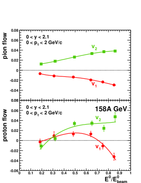
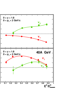
Figure 20: (Color online) Directed and elliptic flow as a function of centrality for charged pions (top) and protons (bottom) from 158$A$ GeV Pb + Pb (left) and 40$A$ GeV Pb + Pb (right) from the standard analysis. Shown are $v_{1}$ (circles) and $v_{2}$ (squares). The more central collisions are on the left side of each graph. Solid lines are polynomial fits.

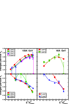
Figure 21: (Color online) Weighted flow $\langle w_{n}e^{in(\phi-\Phi_{RP})}\rangle/\sqrt{\left\langle{w_{n}}^{2}\right\rangle}$, Eq. (17), with $w_{1}=y$ in the center of mass frame and $w_{2}=p_{t}$, from the cumulant method as a function of centrality in 158$A$ GeV Pb + Pb (left) and 40$A$ GeV Pb+Pb (right). The more central collisions are on the left side of each graph. The lines are polynomial fits. The unplotted points could not be obtained or had error bars which were too large.

Figure 21 shows the weighted integrated flow values for charged particles, Eq. (17), from the cumulant method as a function of centrality, up to eight-particle correlations. Contrary to the standard method results, these values were not obtained by averaging the differential values a posteriori. As mentioned in Sec. IV.2, integrated flow is the first outcome of the cumulant method, which is then used to obtain differential values. In particular, this explains why for $v_{2}$ we could derive integrated values from up to eight-particle cumulants, while only four-particle results are available for differential flow. Also for $v_{1}$ we could obtain integrated values from up to four-particle cumulants while only three-particle results are available for differential flow with reasonable error bars.

Please note that the plotted quantity is not $v_{n}$, but a weighted flow $\left\langle w_{n}e^{in(\phi-\Phi_{RP})}\right\rangle/\sqrt{\left\langle{w_{n}}^{2}\right\rangle}$. Since it is only intended as a reference value in the cumulant method, the weights were chosen so as to maximize it, and indeed it is about a factor of 1.2 larger than the standard analysis value because of the weighting.

A striking feature is the consistency between the flow estimates using more than two particles. Thus, in Fig. 21 top left for 158$A$ GeV, $v_{2}\{4\}$, $v_{2}\{6\}$, and $v_{2}\{8\}$ are in agreement within statistical error bars. This is a clear signal that these estimates indeed measure the “true” $v_{2}$, and are all arising from a collective motion. In addition, it is interesting to note that these three estimates differ significantly from the two-particle estimate $v_{2}\{2\}$, which suggests that the latter is contaminated by nonflow effects. This will be further examined in Sec. V.5. Apart from that, these charged particle values follow the usual trend for pions: the absolute value of $v_{1}$ increases in going to more peripheral collisions; $v_{2}$ also increases in going from central to semi-central collisions, but then starts to decrease for the most peripheral bins, both at 40 and 158$A$ GeV.

V.5 Nonflow effects

The purpose of the cumulant method is to remove automatically nonflow effects, so as to isolate flow. Nevertheless, one may wonder whether this removal is really necessary, and if nonflow effects are significant.

A first way to estimate the contribution of nonflow effects, which was proposed in Ref. Borghini:2002vp , consists in plotting the quantity $N\cdot(v_{n}\{2\}^{2}-v_{n}\{k\}^{2})$ as a function of centrality, where $N$ is the mean total number of particles per collision in a given centrality bin, and $k>2$. The reason is that the two-particle estimate $v_{n}\{2\}$ is contaminated by nonflow effects, while the estimate from more particles $v_{n}\{k\}$ is not, hence their difference should be due to the nonflow correlations. More precisely, the two-particle cumulant reads

$$c_{n}\{2\} \equiv v_{n}\{2\}^{2}\,$$ (19)

$$= (v_{n})^{2}+{\rm nonflow}\,$$ (20)

$$= (v_{n})^{2}+\frac{g_{n}}{N},$$ (21)

where we have recalled the definition of the two-particle flow estimate $v_{n}\{2\}$, see Eq. (15), and the nonflow term scales as $1/N$. Since it is hoped that the multi-particle estimates reflect only flow, $v_{n}\simeq v_{n}\{k\}$, a straightforward rearrangement shows that

$$N\cdot(v_{n}\{2\}^{2}-v_{n}\{k\}^{2})=g_{n}$$ (22)

should be approximately constant. Note that $g_{1}$ and $g_{2}$ were calculated directly from the cumulants, not from the values of the flow estimates:

$$g_{1} = N\cdot\left(c_{1}\{2\}-c_{1}\{3\}/v_{2}\right),$$ (23)

$$g_{2} = N\cdot\left(c_{2}\{2\}-\sqrt{-c_{2}\{4\}}\right)$$ (24)

($c_{1}\{3\}$ denotes the left-hand side of Eq. (11), and the other cumulants have been defined in Sec. IV.2). This explains why we can display values for almost all centrality bins, while there might be no corresponding flow values because of a wrong sign for the cumulant . In Fig. 22 are shown the coefficients $g_{1}$ and $g_{2}$ as a function of centrality, for both 158 and 40$A$ GeV, where the values of $N$ are taken from Table 2. The magnitude of the statistical error follows the analytical formulas given in Appendix B.

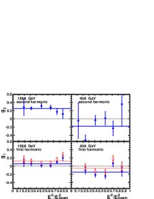
Figure 22: (Color online) Nonflow azimuthal correlations from Eq.(22), for the first, $g_{1}$, (bottom) and second, $g_{2}$, (top) Fourier harmonics, from 158$A$ GeV (left) and 40$A$ GeV (right) Pb+Pb collisions. For $g_{1}$, the solid points represent all nonflow effects, while the open points are corrected for momentum conservation. The horizontal lines are at the mean values.

As could be expected from the fact that in Fig. 21 top left the two-particle points are above the multi-particle points, a clear nonflow signal can be observed in Fig. 22 top left for the second harmonic in full energy collisions. Moreover, $g_{2}$ is approximately constant, as expected for nonflow correlations: one has approximately $v_{2}\{2\}^{2}\simeq v_{2}\{4\}^{2}+0.26/N$, at least for the four more central bins.

For the first harmonic, two types of results are displayed in Fig. 22 bottom: the solid points correspond to all nonflow effects in Eq. (22), while the open points are corrected for momentum conservation. The uncorrected points are approximately constant and close to zero at 158$A$ GeV for all but the most peripheral bin. This is quite surprising since we have seen above that the two-particle $v_{1}\{2\}$ is strongly contaminated by correlations arising from momentum conservation. Actually the contribution of this nonflow effect can be explicitly calculated using Eq. (4) of Ref. Borghini:2002mv :

$$g_{1}^{\rm mom-cons}=-\frac{\left\langle y\,p_{t}\right\rangle^{2}}{\left\langle y^{2}\right\rangle\left\langle{p_{t}}^{2}\right\rangle_{\rm all}}=-\frac{N}{M}f^{2}\,,$$ (25)

where averages are calculated over the phase space covered by the detector, except for the subscript “all” which means that all particles are taken into account, including those that fall outside the detector acceptance. The corresponding quantity $\left\langle{p_{t}}^{2}\right\rangle_{\rm all}$ is estimated from a model calculation, see Table 2. In the second version of the equation, $N$ is the multiplicity over all phase space, $M$ is the multiplicity of detected particles, and $f$ is defined by Eq. (19) of Ref. Borghini:2002mv . Note that for a perfect acceptance, or an acceptance symmetric about midrapidity, $g_{1}^{\rm mom-cons}$ vanishes. As expected, $g_{1}^{\rm mom-cons}$ depends weakly on centrality and its mean value is about $-0.067$ at 158$A$ GeV, and $-0.10$ at 40$A$ GeV. Since the acceptance is better at 158$A$ GeV than at 40$A$ GeV, we expect to get a lower value at that energy, and this is the case indeed. Finally, subtracting this contribution to $g_{1}$ (which amounts to an addition, since $g_{1}^{\rm mom-cons}<0$), all values are shifted upward and we get a clear positive value at 158$A$ GeV for all nonflow effects except momentum conservation.

The important point is that the whole $g_{1}$ is only an integrated quantity, averaged over phase space and summed over different particle types, and variations of opposite sign may cancel. As a matter of fact, we have already noted in Sec. V.2 that for pions the three-particle estimate $v_{1}\{3\}$ is lower than $v_{1}\{2\}$ at large $p_{t}$, but larger at low $p_{t}$ (Fig. 13, left): ascribing the large-momentum discrepancy to momentum conservation, and the low-$p_{t}$ one to short-range correlations, it turns out that they compensate when one averages over $p_{t}$. Similarly, we have already mentioned that the difference seen in the directed flow of protons (Fig. 13, right) between the standard analysis value (corrected for $p_{t}$ conservation) and the three-particle estimate at high momentum could be due to correlations from $\Delta$ decays, an effect that may explain the open points in Fig.22, bottom.

On the contrary, the nonflow correlations in the second harmonic, which are seen in Fig. 22, cannot be localized in any definite region of phase space in Figs. 7 or 8, and thus there is no clue regarding the actual effects which contribute. One may simply notice that the order of magnitude of $g_{2}$ is the same as the estimate for the contribution from $\rho$-meson decays Borghini:2000cm , although resonance decays may only explain part of $g_{2}$. Nevertheless, one can safely conclude that nonflow effects are significant at 158$A$ GeV and play a role in the analysis of both $v_{1}$ and $v_{2}$.

At 40$A$ GeV, Fig. 22 is less conclusive than at 158$A$ GeV, but we have seen in Sec. V clear indications of nonflow correlations. First, we recall that the importance of nonflow effects, and especially of momentum conservation, in the first harmonic is such that it is not possible to obtain directed flow from the two-particle cumulant, $v_{1}\{2\}$, while the standard method (including correction for $p_{t}$ conservation) or the three-particle cumulant do give results. Apart from this large effect, we also mentioned the possible presence of short-range correlations at low $p_{t}$, which could explain why the standard method value for $v_{1}$ does not go smoothly to zero at vanishing momentum, while the three-particle result $v_{1}\{3\}$ does. In the second harmonic, we have seen in Sec. V.1 large discrepancies between the two- and four-particle estimates, in central collisions. As suggested above, the observed differences may arise from two-particle correlations due to $\rho$-meson decays.

V.6 Beam energy dependence

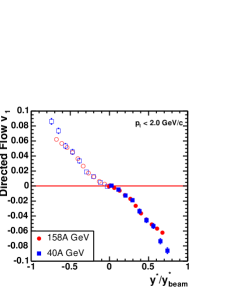
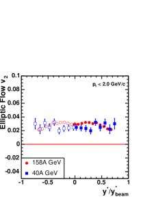
Figure 23: (Color online) A comparison of directed and elliptic flow of charged pions at 40 and 158$A$ GeV using the standard method is shown as a function of scaled rapidity. The left graph for $v_{1}$ is for peripheral collisions and the right graph for $v_{2}$ is for mid-central collisions. The open points have been reflected about midrapidity.

A direct comparison between flow at 40 and 158$A$ GeV is presented in Fig. 23, where $v_{1}$ and $v_{2}$ for pions are plotted as a function of scaled rapidity $y/y_{beam}$. The use of scaled rapidity is justified by the fact that the width of the rapidity distribution of produced hadrons increases approximately as $y_{beam}$ NA49-energy and that the shapes of the transverse momentum distributions are similar at 40 and 158$A$ GeV NA49-energy . Dependence of $v_{1}$ and $v_{2}$ on scaled rapidity is similar for both energies, however there is an indication that $v_{2}$ is slightly larger at 158$A$ GeV than at 40$A$ GeV, although $v_{1}$ appears to be the same at the two beam energies. For $v_{1}$ at the other centralities the agreement is not as close, but the $v_{1}\{3\}$ integrated results, which are free from nonflow effects, agree at the two beam energies.

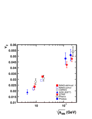
Figure 24: (Color online) Energy dependence of $v_{2}$ near mid-rapidity ($0<y<0.6$ for 40$A$ GeV and $0<y<0.8$ for 158$A$ GeV) for mid-central collisions (approx. 12 to 34 % of geometrical cross section). The results of NA49 pion $v_{2}$ are compared to charged particle $v_{2}$ measured by E877, STAR, PHENIX and PHOBOS.

Elliptic flow was recently measured at midrapidity in Au+Au at RHIC energies Ray:QM02 ; Esumi:QM2002 ; Manly:QM2002 . These measurements together with the corresponding measurements presented in this paper and other SPS measurements CERES:INPC01 ; CERES:QM02 (there are newer measurements not taken into account yet, as they were taken at different centralities CERES:YUN02 ), as well as the measurement at the AGS Voloshin:1999gs , allow us to establish the energy dependence of $v_{2}$ in a broad energy range. The STAR data have been scaled down to take into account the low $p_{t}$ cut-offs of 150 MeV/c at $\sqrt{s_{NN}}=200$ GeV and 75 MeV/c at $\sqrt{s_{NN}}=130$ GeV. The correction factors have been obtained by extrapolating the charged particle yield to zero $p_{t}$ and assuming a linear dependence of $v_{2}(p_{t})$ at small transverse momenta. The factors were 1.14 for the $\sqrt{s_{NN}}=200$ GeV data and 1.06 for the $\sqrt{s_{NN}}=130$ GeV data. The SPS data do not have a low $p_{t}$ cutoff. In Fig. 24 $v_{2}$ at midrapidity is plotted as a function of center of mass energy per nucleon–nucleon pair for mid-central collisions. The rise with beam energy is rather smooth.

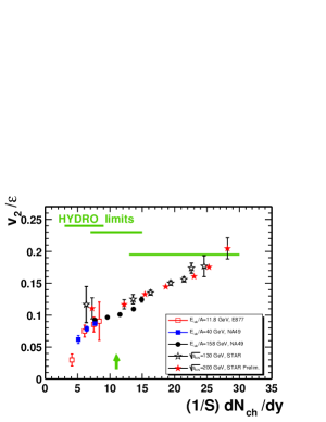
Figure 25: (Color online) $v_{2}/\epsilon$ as a function of particle density. The $v_{2}$ values are for near mid-rapidity ($0<y<0.6$ for 40$A$ GeV and $0<y<0.8$ for 158$A$ GeV). The results of NA49 pion $v_{2}$ are compared to charged particle $v_{2}$ measured by E877 and STAR. The meaning of the horizontal lines (hydro limits) and of the arrow will be discussed in Sec. VI.

$v_{2}$ divided by the initial eccentricity of the overlap region, $\epsilon$, is free from geometric contributions Sorge:1998mk . It is useful to plot this quantity versus the particle density as estimated by $dN/dy$ of charged particles divided by the area of the overlap region, $S$ Voloshin:1999gs ; Voloshin:QM02 . The initial spatial eccentricity is calculated for a Woods-Saxon distribution with a wounded nucleon model from

$$\epsilon=\frac{\langle y^{2}\rangle-\langle x^{2}\rangle}{\langle y^{2}\rangle+\langle x^{2}\rangle}\,$$ (26)

where $x$ and $y$ are coordinates in the plane perpendicular to the beam and $x$ denotes the in-plane direction. Fig. 25 shows our results for $v_{2}\{2\}$ together with the recent STAR results on elliptic flow from 4-particle cumulants STAR:130 ; Ray:QM02 , and E877 results Voloshin:1999gs from the standard method. The RHIC data have been corrected for their low $p_{t}$ cut-off as described for Fig. 24. Only statistical errors are shown.

The NA49 results shown in the figure were obtained with the 2-particle cumulant method. The total systematic uncertainties for the points are unfortunately rather large and amount to about 30% of the presented values. The systematic errors for the most central collisions are even larger and taking into account also the larger statistical errors we do not plot them in the figure. The results obtained for NA49 with the standard method as well as from 4-particle cumulants have larger statistical errors but are within the systematic errors quoted. There are also possible systematic errors of the order of 10-20% due to uncertainties in the centrality measurements from one experiment to the other. Note that the most peripheral RHIC data are slightly above the slightly more central data from the SPS, but would agree within these systematic errors. This slight non-scaling could be related to the use of $\epsilon$ calculated with a weight proportional to the number of wounded nucleons. A different weight could give somewhat different relative values for spatial eccentricities of central and peripheral collisions. In general the figure shows a nice scaling of the elliptic flow divided by the initial spatial eccentricity when plotted against the produced particle density in the transverse plane. The physical interpretation will be discussed in Sec. VI.

The energy dependence of directed flow is also instructive. Directed flow has not yet been seen at RHIC, but it has been extensively studied at lower energies at the AGS. The most striking difference between the present results and AGS results is in the rapidity dependence of the proton directed flow. Up to the top AGS energy, the proton $v_{1}(y)$ follows the well-known S-shape, with a maximum slope at midrapidity Liu:2000am . By contrast, at SPS, already at 40$A$ GeV, the slope at midrapidity is consistent with zero within our errors. This is compatible with a smooth extrapolation of AGS results, which already show a significant decrease of the slope at midrapidity between 2 and 11 $A$ GeV.

While the proton $v_{1}$ near midrapidity becomes much smaller as the energy increases, the pion $v_{1}$ near midrapidity remains of comparable magnitude. The main difference, compared to AGS energies, is that $v_{1}$ remains negative until very high values of $p_{t}$, while at AGS it becomes positive typically above 500 MeV/c Barrette:1997pt , which was interpreted as an effect of the sidewards motion of the source.

VI Model comparisons

Here we review theoretical predictions for elliptic and directed flow at SPS energies and compare them with our results. Note however that detailed predictions have only been made for 158$A$ GeV collisions.

VI.1 Elliptic flow

Elliptic flow at ultrarelativistic energies is interpreted as an effect of pressure in the interaction region. In the transverse plane, particles are created where the two incoming nuclei overlap. This defines a lens-shaped region for non-central collisions. Subsequent interactions between the particles drive collective motion along the pressure gradient, which is larger parallel to the smallest dimension of the lens. This creates in-plane, positive elliptic flow OL92 . At early times, however, spectator nucleons tend to produce negative elliptic flow Sorge:1996pc : while this effect dominates at energies below 5 GeV per nucleon Pinkenburg:1999ya , one expects it to be negligible at SPS energies, except close to the projectile rapidity, which is not covered by the present experiment.

As it is essentially a pressure effect, elliptic flow is sensitive both to the equation of state of nuclear matter (i.e., the relation between pressure and density), and the degree of thermalization reached in the system. The equation of state enters mainly through the velocity of sound, $c_{s}\equiv(dP/d\epsilon)^{1/2}$, which controls the magnitude of pressure gradients: naturally, a “softer” equation of state, with smaller $c_{s}$, produces smaller elliptic flow, and this is true in particular in the presence of a first-order phase transition where $c_{s}$ vanishes OL92 . From a microscopic point of view, elliptic flow increases with the number of collisions per particle: very generally, one expects a linear increase, followed by a saturation when the system reaches thermal equilibrium Molnar:2001ux . Disentangling both effects (equation of state vs. degree of thermalization), however, is far from obvious.

Various predictions have been made for elliptic flow at SPS energies. They are based either on hydrodynamic models, where full thermal equilibrium is assumed, or on transport models, where collisions between particles are treated at a microscopic level. We briefly review these predictions and discuss how they compare with the present data.

Let us start with the transverse momentum dependence of $v_{2}$. As can be seen in Figs. 7 and 10, $v_{2}$ vanishes at low $p_{t}$ and then increases regularly. The dependence is almost linear for pions, but rather quadratic below 1 GeV/$c$ for protons: therefore $v_{2}$ is smaller for protons than for pions at low $p_{t}$, while they become of comparable magnitude at 2 GeV/$c$. These nontrivial features are qualitatively reproduced by hydrodynamical models Kolb:00 ; Kolb:2000fh , where the dependence on the hadron mass is well understood pasi2 . Unfortunately, there do not seem to be any predictions from transport models for $v_{2}(p_{t})$ at SPS energies. Several such calculations are available at the higher RHIC energies, where the same features are observed Bleicher:2000sx ; Lin:2001zk ; Humanic:2002iw ; Sahu:2002sp . Coming to quantitative comparisons, elliptic flow at 158$A$ GeV seems to be overestimated by hydrodynamical calculations, although not by a large factor. Kolb et al. Kolb:00 predict $v_{2}(p_{t}=1\,{\rm GeV}/c)\simeq 12\%$ for pions in mid-central collisions, while our various estimates (see Fig. 7, middle left) are closer to $8\%$. The model of Teaney et al. Teaney:2001av , which couples hydrodynamics to a transport model, naturally yields smaller values of $v_{2}$ (about $10\%$ for pions at $p_{t}=1$ GeV/$c$), but still higher than our data. These hydrodynamical calculations use “soft” equations of state, which are needed in order to reproduce the measured $p_{t}$ spectra. The fact that they tend to overestimate $v_{2}$ suggests that thermalization is only partially achieved even at the top SPS energy.

The rapidity dependence of $v_{2}$ is also instructive. Due to the strong Lorentz contraction at ultrarelativistic energies, all the produced particles essentially originate from the same point $z=t=0$. Therefore, the longitudinal velocity $v_{z}$ of a particle (or its rapidity) is expected to be strongly correlated to its position $z$ throughout the evolution of the system. This means that particles with the same rapidity are those which interacted throughout the evolution. Following the common interpretation of elliptic flow as due to secondary collisions, one expects an increase of $v_{2}$ with the multiplicity density $dN/dy$, up to the limiting value corresponding to thermal equilibrium. It is interesting to note that, at 158$A$ GeV, the rapidity dependence of $v_{2}$ (Fig. 8) follows that of the multiplicity $dN/dy$ crosssections , although it is less pronounced. This again suggests only partial thermalization. Let us now come to quantitative comparisons with the various models. Most of the calculations were done with the same $p_{t}$ cuts as in the earlier NA49 analysis NA49PRL , i.e. $50<p_{t}<350$ MeV/$c$ for pions, which would yield values of $v_{2}(y)$ smaller than in the present analysis by a factor of approximately 2 according to our measurements. First, all above mentioned hydrodynamical calculations assume rapidity independence Bjorken:1982qr , so that they are unable to predict the rapidity dependence of $v_{2}$. Hirano Hirano:2000eu performs a full three-dimensional hydro calculation, tuned to reproduce both rapidity and transverse momentum spectra. The resulting $v_{2}(y)$ is about $3\%$ at midrapidity, significantly larger than our result in Fig. 8, middle left (with due attention to the different cuts in $p_{t}$, as explained above), and the decrease at higher rapidities seems to be steeper than in our data. Various predictions are available from microscopic models for $v_{2}(y)$ of pions and protons at the top SPS energy. Predictions of RQMD Liu:1998yc and UrQMD Soff:1999yg seem to be in agreement with our data, at least qualitatively. Calculations based on the QGSM model Bravina:2000dg show a dip near midrapidity for peripheral collisions, which we do not see in the data.

The centrality dependence of $v_{2}$ is particularly interesting. In hydrodynamics, it closely follows the centrality dependence of the initial asymmetry, i.e., $v_{2}$ is proportional to the eccentricity $\epsilon$ of the lens-shaped object OL92 . It thus increases with impact parameter up to very peripheral collisions if the system is thermalized. On the other hand, if only partial thermalization is achieved, $v_{2}$ is smaller for peripheral collisions, and the maximum of $v_{2}$ is shifted to less peripheral collisions Kolb:2000fh ; Voloshin:1999gs . Since the eccentricity of the lens-shaped object, $\epsilon$, increases linearly with the number of spectator nucleons OL92 , one would expect a linear increase of $v_{2}$ with $E^{0}$ in Figs. 20 and 21. At 158$A$ GeV, the experimental curve clearly bends over in the two most peripheral bins, and this tendency is more pronounced with estimates from higher order cumulants which are less sensitive to nonflow correlations. This again suggests that thermalization is not fully achieved. At 40$A$ GeV, error bars are larger, but the decrease of $v_{2}$ is even more pronounced in the most peripheral bin: departure from thermalization would then be more important than at the higher energy, which is to be expected since the density is lower. Finally, a peculiar centrality dependence of $v_{2}$ was proposed as a signature of the phase transition to the quark-gluon plasma Sorge:1998mk : with increasing centrality (i.e. decreasing impact parameter), the ratio $v_{2}/\epsilon$ was predicted to first increase, due to better thermalization, then saturate, and eventually increase again for the most central collisions as a result of the re-hardening of the equation of state when a quark-gluon plasma is produced. At 158$A$ GeV, however, Fig. 21 shows that the increase of $v_{2}$ with the number of spectators is linear for the most central collisions, which suggests a constant $v_{2}/\epsilon$. At 40$A$ GeV, on the other hand, the flow obtained from 4-particle cumulants remains unusually high for central collisions, which may be a hint of interesting physics.

We finally come to the dependence of $v_{2}$ on beam energy. There are very few model calculations of $v_{2}$ at 40$A$ GeV in the literature. The most natural expectation is that $v_{2}$ should increase regularly as the beam energy increases, and eventually saturate: first, because the effect of spectators (which tends to lower $v_{2}$) decreases, second, because the degree of thermalization increases. Such a behavior is indeed observed with a smoothly varying equation of state Kolb:99 . If a strong first order phase transition occurs in the system, however, an interesting structure is predicted Kolb:99 , where a small maximum in $v_{2}$ occurs somewhere between the top AGS and the top SPS energies. Such a structure does not appear in Fig. 24, which shows that the increase of $v_{2}$ from AGS to RHIC is smooth.

There is a nice way to combine the centrality dependence and the beam energy dependence of $v_{2}$, by plotting the scaled anisotropy $v_{2}/\epsilon$ versus the particle density as estimated by $dN/dy$ of charged particles divided by the area of the overlap region, $S$ Voloshin:1999gs ; Voloshin:QM02 . If the system is locally thermalized, and if there is no marked structure in the equation of state (such as a strong first order phase transition), $v_{2}/\epsilon$ is expected to be centrality independent as explained above, and to depend only weakly on the beam energy through the equation of state: this is indicated by the horizontal lines (“hydro limits”) in Fig. 25. If the mean free path of the particles becomes as large as the transverse size, thermalization is not reached, and $v_{2}/\epsilon$ is smaller than the hydro limit: it is expected to increase smoothly with the ratio between the transverse size and the mean free path, and eventually saturate at the hydro limit. The latter ratio scales itself like the charged particle density per unit transverse area $(1/S)dN/dy$, which is the abscissa in Fig. 25. The data shown in this figure are compatible with the above picture, since data taken at different beam energies fall on the same universal curve. It is quite remarkable, and far from obvious, that this simple physical picture allows us to compare quantitatively a peripheral collision at the full RHIC energy with a central collision at the lower SPS energy.

A further interest in this plot is the speculation Voloshin:1999gs whether there is flattening at an abscissa value of about 10 which could indicate a change in the physics of rescattering and suggest a deconfinement phase transition in this region. It is noteworthy that the color percolation point Satz:QM02 , which is shown by an arrow in the figure, is just in the same region. Unfortunately, taking into account the large systematic errors of the results, we are not able to resolve this question. Further data analysis at 80$A$ GeV SPS and $\sqrt{s_{NN}}=20$GeV RHIC beam energies would be useful.

VI.2 Directed flow

Elliptic flow at SPS is created by the interactions between the produced particles, but is to a large extent independent of the mechanism of particle production. By contrast, the physics of directed flow probes a time scale set by the crossing time of the Lorentz-contracted nuclei Bleicher:2002xx . It is therefore more subtle, and more strongly model dependent than the physics of elliptic flow.

Directed flow defines the impact parameter as an oriented arrow in the transverse plane. As such, it reflects the asymmetry between target and projectile (to which elliptic flow is insensitive). For this reason, most model calculations only address the directed flow of nucleons. In addition, most papers do not deal with $v_{1}$, but with the mean transverse momentum projected on the reaction plane, $\left\langle p_{x}\right\rangle=\left\langle p_{t}\,v_{1}(p_{t},y)\right\rangle$, as a function of rapidity, for historical reasons Danielewicz:hn .

It was first expected that directed flow would be negligible at SPS energies. In 1991, it was predicted et al. Amelin:cs that it might however be large enough to be measurable in Pb-Pb collisions. Non-zero $v_{1}$ for nucleons was predicted both by a transport model (QGSM) including re-scatterings, and by a hydrodynamical model. Furthermore, in the hydro model, $\left\langle p_{x}\right\rangle$ depended strongly on the equation of state: as elliptic flow, directed flow is smaller with a softer equation of state (involving for instance a phase transition to a quark-gluon plasma).

The interest in directed flow was revived following the prediction that the “softest point” of the equation of state could be directly observed at the AGS  Hung:1994eq . A deep minimum of $\left\langle p_{x}\right\rangle$ may appear, at an energy of about 6 $A$ GeV Rischke:1995pe . These predictions, however, crucially rely on the assumption that the early stages of the collision, when particles are produced, can be described by one-fluid hydrodynamics. A two-fluid model Ivanov:2000dr predicts no minimum as energy increases. In a three-fluid model Brachmann:1999xt , on the other hand, a minimum occurs, but at a higher energy, around 10-20 GeV per nucleon. It is followed by an increase up to a maximum at 40$A$ GeV. Unfortunately, no quantitative estimate is provided. A similar structure is predicted in the transport model UrQMD Bleicher:2002xx , where the minimum of $\left\langle p_{x}\right\rangle$ also appears as a consequence of the softening of the equation of state (although no quark-gluon plasma is explicitly incorporated in the model): $\left\langle p_{x}\right\rangle$ increases from the top AGS energy and then saturates above 40 GeV per nucleon at a value of $30$ MeV/$c$. Unfortunately, an observable such as $\left\langle p_{x}\right\rangle$ is largest in the target and projectile rapidity regions, which are not covered by the present experiment, so that quantitative comparisons are not possible.

We therefore concentrate on predictions for differential flow as a function of rapidity, $v_{1}(y)$. The remarkable feature of our data in Figs. 14 and 17 is the flatness of $v_{1}$ for protons near mid-rapidity, where the slope at midrapidity may even be negative for peripheral collisions. This “antiflow,” or “wiggle,” was predicted at RHIC energies Snellings:1999bt . It is also present at SPS energies in most fluid-dynamical calculations Brachmann:1999xt ; Csernai:1999nf ; Ivanov:2000dr . Transport models like UrQMD Soff:1999yg predict a too large value of $v_{1}(y)$ for protons, although they do see some flattening near midrapidity. In the QGSM model Bravina:2000dg , $v_{1}(y)$ for protons shows no flattening, except for peripheral collisions. The value of $v_{1}$ of protons is much larger than our data: about 7% for central collisions and 10% for mid-central collisions at $y=1.5$, while we see at most 2%. The value of $v_{1}(p_{t})$ in QGSM Zabrodin:2000xc is also larger than our data for protons.

There are comparatively very few studies of pion directed flow at SPS energies. Pion directed flow was first seen in asymmetric collisions Gosset:1988cm at lower energies. The $v_{1}$ of pions usually has a sign opposite to the proton $v_{1}$, which is understood as an effect of shadowing and absorption on nucleons Bass:em ; Li:tj . The same effect was observed at AGS Barrette:1996rs and is clearly seen in all our data. UrQMD Soff:1999yg correctly predicts $v_{1}(y)$ for pions at the top SPS energy, although their prediction for protons is too high. In the QGSM model Bravina:2000dg , the pion $v_{1}(y)$ has a minimum at about half the projectile rapidity. In Fig. 14, the same tendency is seen in the standard analysis (also quantitative agreement) but not in the three-particle estimate which shows further decrease toward projectile rapidities. The peculiar transverse momentum dependence of $v_{1}$ for pions, which is negative at low $p_{t}$ and then positive above 1 GeV/$c$ (see Figs. 13 and 16), does not seem to have been predicted.

VII Summary

We have presented a true multiparticle analysis of directed and elliptic flow which provides results on $v_{1}$ and $v_{2}$ values of pions and protons as function of rapidity, transverse momentum, collision centrality and beam energy (40 and 158$A$ GeV).

Two independent analyses were carried out using two different methods: the standard method of correlating particles with an event plane, and the cumulant method of studying genuine multiparticle correlations. The cumulant method yields several independent estimates of the flow. From the point of view of physics, the lowest-order estimates $v_{1}\{2\}$, $v_{2}\{2\}$ are essentially equivalent to the estimates from the event-plane method, while higher-order estimates $v_{1}\{3\}$, $v_{2}\{4\}$ are hopefully free from nonflow effects. This is the main motivation of the cumulant method. The two methods are very different in their practical implementation. The cumulant method no longer requires one to construct subevents, or to correct for the event-plane resolution. All flow estimates are derived from a single generating function of azimuthal correlations. Constructing this generating function, however, requires more computer time than the standard flow analysis. Another significant difference between the two methods is that the cumulant method takes naturally into account azimuthal asymmetries in the detector acceptance. Hence the flattening procedures, and the cuts in phase space which are required in the event-plane method in order to minimize the effects of these asymmetries, are no longer required. The price to pay for all these enhancements is increased statistical errors.

We have obtained the first direct, quantitative evidence for collective motion at these energies: elliptic flow at 158$A$ GeV has been reconstructed independently from genuine 4, 6 and 8-particle correlations, and all three results agree within statistical errors (Fig. 21, top left). This is confirmed at both energies by differential analyses of elliptic flow (as a function of rapidity or transverse momentum) from genuine 4-particle correlations. In the case of directed flow, nonflow correlations due to momentum conservation, which are large, have been subtracted. Furthermore, a new method of analysis from 3-particle correlations, which is unbiased by nonflow correlations, has been implemented for the first time at both energies.

The directed flow of protons reveals a structure which is characteristic of ultrarelativistic energies, and is not present at AGS energies. A clear separation appears for the first time between the central rapidity region, where the proton $v_{1}$ is essentially zero, and the target-projectile fragmentation region, where it is large. Indeed, at 40$A$ GeV, significant directed flow is observed only at the most forward rapidities covered by the detector acceptance (Fig. 17, right). At 158$A$ GeV, where the acceptance covers smaller values of the scaled rapidity, $v_{1}$ values are consistent with zero (Fig. 14, right), within statistical errors and possible contributions by nonflow effects. In the fragmentation region, on the other hand, large $v_{1}$ values have been observed by WA98 WA98:QM99 . At both energies, the first observation of the “wiggle” (i.e., a negative slope of the proton $v_{1}$ near mid-rapidity) is reported, but there are indications that it may be due to nonflow effects.

Surprisingly, the directed flow of pions does not follow the same behavior as that of protons. While the proton $v_{1}$ at central rapidity is much smaller than at AGS energies, the pion $v_{1}$ remains essentially of the same magnitude. It becomes even larger, in absolute value, than the proton $v_{1}$. This amazing phenomenon, which has never been observed at lower energies, clearly indicates that the proton $v_{1}$ and the pion $v_{1}$ have different physical origins. The directed flow of pions behaves similarly at the two beam energies, both in magnitude and in shape. It has a peculiar, essentially flat, transverse momentum dependence (Figs. 13 and 16, left). Its centrality dependence is also quite remarkable: it increases in magnitude steadily without saturating up to the most peripheral collisions. (Fig. 20, top, and Fig. 21, bottom).

Elliptic flow becomes the dominant azimuthal anisotropy at ultrarelativistic energies. While it is smaller than directed flow up to the top AGS energy, here it becomes larger already at 40$A$ GeV. This is again an indication that SPS is probing the truly ultrarelativistic regime. As a consequence of the larger value, our estimates of $v_{2}$ are more accurate than our estimates of $v_{1}$. As a function of transverse momentum, $v_{2}$ increases almost linearly for pions, and more quadratically for protons, as already seen at RHIC. On the other hand, the rapidity dependences are the same for pions and protons: $v_{2}$ is approximately constant in the central rapidity region (see e.g., Fig. 8, middle) and drops in the target-projectile fragmentation regions, roughly where the proton $v_{1}$ starts increasing. At 158$A$ GeV, $v_{2}$ has a pronounced centrality dependence (Figs. 20 and 21, left) but, unlike directed flow, it saturates for very peripheral collisions. The centrality dependence at 40$A$ GeV (Figs. 20 and 21, right) is less significant. For protons (shown in the same figures) the tendencies are the same, but the significance is reduced due to larger statistical errors.

The energy dependence of $v_{2}$ looks roughly linear from AGS up to RHIC energies (Fig. 24). No indication of non-monotonic behavior is visible, as would be expected from the softening of the equation of state for a system close to the critical temperature. The dependence of elliptic flow (divided by the eccentricity of the nuclear overlap region) on particle (rapidity) density also exhibits a smooth increase without significant structure (Fig. 25) which would indicate a change in the physics of rescattering.

Appendix A Interpolation formulas for the cumulants

In this appendix, we give interpolation formulas which were used to extract the cumulants of multiparticle correlations up to eight-particle correlations. Following the procedure proposed in Ref. Borghini:2001vi , we introduce interpolation points $z_{p,q}=x_{p,q}+iy_{p,q}$,

$$x_{p,q} \equiv r_{0}\sqrt{p}\,\cos\left(\frac{2\,q\,\pi}{9}\right),$$ (27)

$$y_{p,q} \equiv r_{0}\sqrt{p}\,\sin\left(\frac{2\,q\,\pi}{9}\right),$$ (28)

for $p=1,\cdots,4$, $q=0,\cdots,8$, and $r_{0}$ of order unity. The generating function of cumulants Eq. (13) is then computed at these various points: $C_{p,q}\equiv{\cal C}_{n}(z_{p,q})$, and averaged

$$C_{p}\equiv\frac{1}{9}\sum_{q=0}^{8}C_{p,q}.$$ (29)

Finally, the cumulants for correlations of 2, 4, 6, and 8 particles are given by

$$\displaystyle c_{n}\{2\} = \frac{1}{r_{0}^{2}\left\langle w_{n}^{2}\right\rangle}\left(4\,C_{1}-3\,C_{2}+\frac{4}{3}C_{3}-\frac{1}{4}C_{4}\right),$$ (30)

$$\displaystyle c_{n}\{4\} = \frac{1}{r_{0}^{4}\left\langle w_{n}^{2}\right\rangle^{2}}\left(\frac{-52}{3}C_{1}+19\,C_{2}-\frac{28}{3}C_{3}+\frac{11}{6}C_{4}\right),$$ (31)

$$\displaystyle c_{n}\{6\} = \frac{6}{r_{0}^{6}\left\langle w_{n}^{2}\right\rangle^{3}}\left(9\,C_{1}-12\,C_{2}+7\,C_{3}-\frac{3}{2}C_{4}\right),$$ (32)

$$\displaystyle c_{n}\{8\} = \frac{96}{r_{0}^{8}\left\langle w_{n}^{2}\right\rangle^{4}}\left(-C_{1}+\frac{3}{2}C_{2}-C_{3}+\frac{1}{4}C_{4}\right).$$ (33)

Appendix B Statistical errors of the contribution of nonflow effects

In this appendix, we derive the statistical uncertainties on the coefficients $g_{n}$ in Eqs. (23), using the analytical formulas for the statistical errors of the various estimates $v_{n}\{k\}$ given in Refs. Borghini:2001vi ; Borghini:2002vp .

Let us start with $g_{2}$, that measures nonflow correlations in the second harmonic. We recall its definition:

$$g_{2} \equiv N\cdot\left(c_{2}\{2\}-\sqrt{-c_{2}\{4\}}\right),$$ (34)

$$= N\cdot\left(v_{2}\{2\}^{2}-v_{2}\{4\}^{2}\right),$$ (35)

where the second line holds provided $c_{2}\{4\}$ has the right, negative sign. The statistical error of $g_{2}$ can easily be calculated and reads

$$\left(\delta g_{2}\right)^{2}=4N^{2}\,v_{2}^{2}\left[(\delta v_{2}\{2\})^{2}+(\delta v_{2}\{4\})^{2}-2\left(\left\langle v_{2}\{2\}v_{2}\{4\}\right\rangle-\left\langle v_{2}\{2\}\right\rangle\left\langle v_{2}\{4\}\right\rangle\right)\right].$$ (36)

where we used $\delta(v_{n}^{2})=2v_{n}\delta v_{n}$. Note that since $v_{2}\{2\}$ and $v_{2}\{4\}$ are slightly correlated if they measure an existing $v_{2}$, the error is smaller than the mere geometrical mean of the uncertainties on each flow estimate. Using formulas given in Ref. Borghini:2001vi , we obtain

$$\delta g_{2}=\frac{N}{M}\,\frac{1}{\sqrt{N_{\rm evts}}}\,\frac{\sqrt{1+4{\chi_{2}}^{2}+2{\chi_{2}}^{4}}}{{\chi_{2}}^{2}}\,,$$ (37)

where $N$ is the total number of emitted particles, $M$ the multiplicity used in the analysis, $N_{\rm evts}$ the total number of events and ${\chi_{2}}=v_{2}\sqrt{M}$ the resolution parameter. The estimate of $v_{2}$ from 4-particle cumulants, $v_{2}\{4\}$, was used to calculate $\chi_{2}$.

Eq. (37) is valid as long as relative errors on both 2-particle and 4-particle cumulants are small. When relative errors become large (usually for central collisions where $v_{2}$ is small, or for the most peripheral collisions where $M$ is small), it may happen that the cumulant $c_{2}\{4\}$ is positive, so that $g_{2}$ in Eq. (34) is undefined. In this case, we set our 4-particle estimate $v_{2}\{4\}$ to zero in the second line of Eq. (34). We then estimate the statistical error noting that it is essentially dominated by that on the 4-particle cumulant $c_{2}\{4\}$, which is $\delta c_{2}\{4\}=2/\left(M^{2}\sqrt{N_{\rm evts}}\right)$Borghini:2001vi when the resolution parameter $\chi_{2}$ is small. The statistical error of $g_{2}$ then reads

$$\delta g_{2}=N\sqrt{\delta c_{2}\{4\}}=\frac{N\sqrt{2}}{M\,N_{\rm evts}^{1/4}}.$$ (38)

Consider now $g_{1}$, that is, nonflow correlations in the first harmonic. We may assume that $c_{1}\{2\}$ and $c_{1}\{3\}$ are uncorrelated since the latter comes from a mixed correlation. Therefore, the statistical error of $g_{1}$ can be written as

$$\left(\delta g_{1}\right)^{2}=N^{2}\left[(\delta c_{1}\{2\})^{2}+\frac{(\delta c_{1}\{3\})^{2}}{v_{2}^{2}}+\left(\frac{c_{1}\{3\}}{{v_{2}}^{2}}\,\delta v_{2}\right)^{2}\right].$$ (39)

If the estimated $v_{1}\{3\}$ is reconstructed from $v_{2}\{4\}$, as is the case in the 158$A$ GeV analysis, one should use the statistical error $\delta v_{2}\{4\}$ in Eq. (39). However, at 40$A$ GeV, since we used $v_{2}\{2\}$ (see Sec. IV.2) we have to use $\delta v_{2}\{2\}$ in Eq. (39). The corresponding formulas are given in Borghini:2001vi , while the formula for $\delta c_{1}\{3\}$ can be found in Ref. Borghini:2002vp .

References

- (1) S. Voloshin and Y. Zhang, Z. Phys. C 70, 665 (1996) [arXiv:hep-ph/9407282].
- (2) W. Reisdorf and H. G. Ritter, Ann. Rev. Nucl. Part. Sci. 47, 663 (1997).
- (3) J.-Y. Ollitrault, Phys. Rev. D 46, 229 (1992).
- (4) D. H. Rischke, Nucl. Phys. A 610, 88c (1996) [arXiv:nucl-th/9608024].
- (5) J.-Y. Ollitrault, Nucl. Phys. A 638, 195c (1998) [arXiv:nucl-ex/9802005].
- (6) P. Danielewicz, Nucl. Phys. A 661, 82c (1999) [arXiv:nucl-th/9907098].
- (7) P. F. Kolb, J. Sollfrank, and U. Heinz, Phys. Lett. B 459, 667 (1999) [arXiv:nucl-th/9906003].
- (8) P. F. Kolb, J. Sollfrank, and U. Heinz, Phys. Rev. C 62, 054909 (2000) [arXiv:hep-ph/0006129].
- (9) D. Teaney, J. Lauret, and E. V. Shuryak, Phys. Rev. Lett. 86, 4783 (2001) [arXiv:nucl-th/0011058].
- (10) J. Bächler et al. [NA49 Collaboration], Searching for QCD Phase Transition, Addendum–1 to Proposal SPSLC/P264, CERN/SPSC 97 (1997).
- (11) S. V. Afanasiev et al. [NA49 Collaboration], Phys. Rev. C 66, 054902 (2002) [arXiv:nucl-ex/0205002].
- (12) M. Gaździcki and M. I. Gorenstein, Acta Phys. Polon. B 30, 2705 (1999) [arXiv:hep-ph/9803462].
- (13) H. Appelshäuser et al. [NA49 Collaboration], Phys. Rev. Lett. 80, 4136 (1998) [arXiv:nucl-ex/9711001]; A. M. Poskanzer, Nucl. Phys. A 638, 463c (1998).
- (14) http://na49info.cern.ch/na49/Archives/Images/Publications/Phys.Rev.Lett.80:4136-4140,1998/ .
- (15) A. M. Poskanzer et al. [NA49 Collaboration], Nucl. Phys. A 661, 341c (1999) [arXiv:nucl-ex/9906013].
- (16) A. Wetzler et al. [NA49 Collaboration], Quark Matter ’02, Nucl. Phys. A 715, 583c (2003) [arXiv:nucl-ex/0212023].
- (17) N. Borghini, P.M. Dinh, and J.-Y. Ollitrault, Quark Matter ’02, Nucl. Phys. A 715, 629c (2003) [arXiv:nucl-th/0208014].
- (18) P. Danielewicz and G. Odyniec, Phys. Lett. B 157, 146 (1985).
- (19) J.-Y. Ollitrault, [arXiv:nucl-ex/9711003].
- (20) A. M. Poskanzer and S. A. Voloshin, Phys. Rev. C 58, 1671 (1998) [arXiv:nucl-ex/9805001].
- (21) P. M. Dinh, N. Borghini, and J.-Y. Ollitrault, Phys. Lett. B 477, 51 (2000);
- (22) N. Borghini, P. M. Dinh, and J.-Y. Ollitrault, Phys. Rev. C 62, 034902 (2000).
- (23) N. Borghini, P. M. Dinh, J.-Y. Ollitrault, A.M. Poskanzer, and S.A. Voloshin, Phys. Rev. C 66, 014901 (2002) [arXiv:nucl-th/0202013].
- (24) N. Borghini, P. M. Dinh and J. Y. Ollitrault, Phys. Rev. C 63, 054906 (2001) [arXiv:nucl-th/0007063].
- (25) N. Borghini, P. M. Dinh, and J.-Y. Ollitrault, Phys. Rev. C 64, 054901 (2001) [arXiv:nucl-th/0105040]; see also Proceedings of the International Workshop on the Physics of the Quark-Gluon Plasma, Ecole Polytechnique, Palaiseau, France, p. 237 (2001) [arXiv:nucl-ex/0110016].
- (26) N. Borghini, P. M. Dinh, and J.-Y. Ollitrault, Phys. Rev. C 66, 014905 (2002), [arXiv:nucl-th/0204017].
- (27) S. Afanasev et al. [NA49 Collaboration], Nucl. Instrum. Meth. A 430, 210 (1999).
- (28) H. Appelshäuser et al. [NA49 Collaboration], Eur. Phys. J. A2, 383 (1998).
- (29) K. H. Ackermann et al. [STAR Collaboration], Phys. Rev. Lett. 86, 402 (2001) [arXiv:nucl-ex/0009011].
- (30) J.-Y. Ollitrault, Phys. Rev. D 48, 1132 (1993) [arXiv:hep-ph/9303247].
- (31) N. Borghini, arXiv:hep-ph/0302139.
- (32) G. E. Cooper, PhD thesis, University of California at Berkeley, 2000 [LBNL-45467, http://na49info.cern.ch/cgi-bin/wwwd-util/NA49/NOTE?222]; G. E. Cooper [NA49 Collaboration], Nucl. Phys. A661, 362c (1999).
- (33) C. Adler et al. [STAR Collaboration], Phys. Rev. Lett. 87, 182301 (2001) [arXiv:nucl-ex/0107003].
- (34) P. Huovinen, P. F. Kolb, U. W. Heinz, P. V. Ruuskanen, and S. A. Voloshin, Phys. Lett. B 503, 58 (2001) [arXiv:hep-ph/0101136].
- (35) R. Snellings [the STAR Collaboration], arXiv:nucl-ex/0305001.
- (36) M. M. Aggarwal et al. [WA98 Collaboration], [arXiv:nucl-ex/9807004].
- (37) R. J. Snellings, H. Sorge, S. A. Voloshin, F. Q. Wang, and N. Xu, Phys. Rev. Lett. 84, 2803 (2000) [arXiv:nucl-ex/9908001].
- (38) S. A. Voloshin, Quark Matter ’02, Nucl. Phys. A 715, 379c (2003) [arXiv:nucl-ex/0210014].
- (39) L. Ray, Quark Matter ’02, Nucl. Phys. A 715, 45c (2003) [arXiv:nucl-ex/0211030].
- (40) S. Esumi et al. [PHENIX Collaboration], Quark Matter ’02, Nucl. Phys. A 715, 599c (2003) [arXiv:nucl-ex/0210012].
- (41) S. Manly et al. [PHOBOS Collaboration], Quark Matter ’02, Nucl. Phys. A 715, 611c (2003) [arXiv:nucl-ex/0210036].
- (42) K. Filimonov et al. [CERES Collaboration], International Nuclear Physics Conference, Berkeley, (2001) [arXiv: nucl-ex/0109017] and private communication.
- (43) J. Slivova [CERES Collaboration], Quark Matter ’02, Nucl. Phys. A 715, 615c (2003) [arXiv:nucl-ex/0212013].
- (44) S.I.Esumi, J. Slivova, J. Milosevic for CERES Collaboration SFIN, year XV, Series A: Conferences, No. A2(2002)
- (45) H. Liu et al. [E895 Collaboration], Phys. Rev. Lett. 84, 5488 (2000) [arXiv:nucl-ex/0005005].
- (46) J. Barrette et al. [E877 Collaboration], collisions at 11-A-GeV/c,” Phys. Rev. C 56, 3254 (1997) [arXiv:nucl-ex/9707002].
- (47) H. Sorge, Phys. Rev. Lett. 82, 2048 (1999) [arXiv:nucl-th/9812057].
- (48) S. A. Voloshin and A. M. Poskanzer, Phys. Lett. B 474, 27 (2000) [arXiv:nucl-th/9906075].
- (49) C. Adler et al. [STAR Collaboration], Phys. Rev. C 66, 034904 (2002) [arXiv:nucl-ex/0206001].
- (50) H. Satz, Quark Matter ’02, Nucl. Phys. A 715, 3c (2003) [arXiv:hep-ph/0209181].
- (51) H. Schlagheck [WA98 Collaboration], Quark Matter ’99, Nucl. Phys. A661 337c (1999). [arXiv:nucl-ex/9907005].
- (52) H. Sorge, Phys. Rev. Lett. 78, 2309 (1997) [arXiv:nucl-th/9610026].
- (53) C. Pinkenburg et al. [E895 Collaboration], Phys. Rev. Lett. 83, 1295 (1999) [arXiv:nucl-ex/9903010].
- (54) D. Molnar and M. Gyulassy, Nucl. Phys. A 697, 495 (2002) [Erratum-ibid. A 703, 893 (2002)] [arXiv:nucl-th/0104073].
- (55) P. F. Kolb, P. Huovinen, U. W. Heinz, and H. Heiselberg, Phys. Lett. B 500, 232 (2001) [arXiv:hep-ph/0012137].
- (56) M. Bleicher and H. Stöcker, Phys. Lett. B 526, 309 (2002) [arXiv:hep-ph/0006147].
- (57) Z. w. Lin and C. M. Ko, Phys. Rev. C 65, 034904 (2002) [arXiv:nucl-th/0108039].
- (58) T. J. Humanic, [arXiv:nucl-th/0205053].
- (59) P. K. Sahu, N. Otuka, and A. Ohnishi, [arXiv:nucl-th/0206010].
- (60) D. Teaney, J. Lauret, and E. V. Shuryak, [arXiv:nucl-th/0110037].
- (61) J. D. Bjorken, Phys. Rev. D 27, 140 (1983).
- (62) T. Hirano, Phys. Rev. Lett. 86, 2754 (2001) [arXiv:nucl-th/0004029].
- (63) H. Liu, S. Panitkin, and N. Xu, Phys. Rev. C 59, 348 (1999) [arXiv:nucl-th/9807021].
- (64) S. Soff, S. A. Bass, M. Bleicher, H. Stöcker, and W. Greiner, [arXiv:nucl-th/9903061].
- (65) L. V. Bravina, A. Faessler, C. Fuchs, and E. E. Zabrodin, Phys. Rev. C 61, 064902 (2000) [arXiv:nucl-th/0002045].
- (66) M. Bleicher and J. Aichelin, [arXiv:nucl-th/0205069].
- (67) N. S. Amelin, E. F. Staubo, L. P. Csernai, V. D. Toneev, K. K. Gudima, and D. Strottman, Phys. Rev. Lett. 67, 1523 (1991).
- (68) C. M. Hung and E. V. Shuryak, Phys. Rev. Lett. 75, 4003 (1995) [arXiv:hep-ph/9412360].
- (69) D. H. Rischke, Y. Pursun, J. A. Maruhn, H. Stöcker, and W. Greiner, Heavy Ion Phys. 1, 309 (1995) [arXiv:nucl-th/9505014].
- (70) Y. B. Ivanov, E. G. Nikonov, W. Noerenberg, A. A. Shanenko, and V. D. Toneev, [arXiv:nucl-th/0011004].
- (71) J. Brachmann et al., Phys. Rev. C 61, 024909 (2000) [arXiv:nucl-th/9908010]; J. Brachmann, A. Dumitru, H. Stöcker, and W. Greiner, Eur. Phys. J. A 8, 549 (2000) [arXiv:nucl-th/9912014].
- (72) L. P. Csernai and D. Röhrich, Phys. Lett. B 458, 454 (1999) [arXiv:nucl-th/9908034].
- (73) E. E. Zabrodin, C. Fuchs, L. V. Bravina, and A. Fässler, Phys. Rev. C 63, 034902 (2001) [arXiv:nucl-th/0006056].
- (74) J. Gosset et al., Phys. Rev. Lett. 62, 1251 (1989).
- (75) S. A. Bass, R. Mattiello, H. Stöcker, W. Greiner, and C. Hartnack, Phys. Lett. B 302 (1993) 381.
- (76) B. A. Li, Nucl. Phys. A 570, 797 (1994).
- (77) J. Barrette et al. [E877 Collaboration], Phys. Rev. C 55, 1420 (1997) [arXiv:nucl-ex/9610006].