Single Identified Hadron Spectra from $\sqrt{s_{NN}}=130$ GeV Au+Au Collisions

Abstract

Transverse momentum spectra and yields of hadrons are measured by the PHENIX collaboration in Au + Au collisions at $\sqrt{s_{NN}}=130$ GeV at the Relativistic Heavy Ion Collider (RHIC). The time-of-flight resolution allows identification of pions to transverse momenta of 2 GeV/c and protons and antiprotons to 4 GeV/c. The yield of pions rises approximately linearly with the number of nucleons participating in the collision, while the number of kaons, protons, and antiprotons increases more rapidly. The shape of the momentum distribution changes between peripheral and central collisions. Simultaneous analysis of all the $p_{T}$ spectra indicates radial collective expansion, consistent with predictions of hydrodynamic models. Hydrodynamic analysis of the spectra shows that the expansion velocity increases with collision centrality and collision energy. This expansion boosts the particle momenta, causing the yield from soft processes to exceed that for hard to large transverse momentum, perhaps as large as 3 GeV/c.

I INTRODUCTION

Heavy ion reactions at ultrarelativistic energies provide information on strongly interacting matter under extreme conditions. Lattice QCD and phenomenological predictions indicate that at high enough energy density a deconfined state of quarks and gluons, the quark-gluon-plasma, is formed. It is expected that conditions in ultrarelativistic heavy ion reactions may produce this new state of matter, the study of which is the major goal of the experiments at the Relativistic Heavy Ion Collider (RHIC).

The high energy density state thus created will cool down and expand, undergoing a phase transition to “ordinary” hadronic matter. While the tools of choice to study the earliest phase of the reactions, and thereby the new state, are probes that do not interact via the strong force, such as photons, electrons, or muons, the global properties and dynamics of later stages in the system are best studied via hadronic observables. Hadron momentum spectra in proton-proton reactions are often separated into two parts, a soft part at low transverse momentum ($p_{T}$), where the shape is roughly exponential in transverse mass $m_{T}=\sqrt{p_{T}^{2}+m_{0}^{2}}$, and a high $p_{T}$ region where the shape more closely resembles a power law. Soft production (low $p_{T}$) is attributed to fragmentation of a string Andersson et al. (1983); Artru (1983) between components of the struck nucleons, while hard (high $p_{T}$) hadrons are expected to originate predominantly from fragmentation of hard-scattered partons. The transition between these two regimes is not sharply defined, but is commonly believed to be near $p_{T}\approx$ 2 GeV/c Owens et al. (1978).

In proton-nucleus (p+A) scattering, these two regimes depend on the colliding system size in different ways. The soft production depends on the number of nucleons struck, or participating in the collision ($N_{part}$). The number of hard scatterings should increase proportionally to the number of binary nucleon-nucleon encounters ($N_{coll}$) since these processes have a small elementary cross section and may be considered as incoherent. Hard scattering also produces color strings which fragment and produce some low $p_{T}$ particles, though these are much fewer in number than those from the much more frequent soft scatterings. In p+A these $N_{part}$ and $N_{coll}$ are connected by a very simple relation, namely $N_{part}=N_{coll}+1$.

In nucleus-nucleus collisions, the number of participant nucleons does not scale simply with A, so it is more useful to study scaling with $N_{coll}$ or $N_{part}$. Collisions are sorted according to centrality, allowing control of the geometry and determination of $N_{coll}$ or $N_{part}$.

In heavy ion collisions, one expects secondary collisions of particles (rescattering) to take place, especially among particles with low and intermediate transverse momentum. Rescattering may occur among partons early in the collision, and also among hadrons later in the collision. Both kinds of rescattering can lead to collective behavior among the particles, and the presence of elliptic flow (Ackermann et al. (2001); Adler et al. (2001a, 2002, 2003); Adcox et al. (2002a); Back et al. (2002a)) indicates that partonic rescattering is important at RHIC. In the extreme, rescattering can lead to thermalization. Rescattering has observable consequences on the final hadron momentum spectra, causing them to be broadened as shown in this paper. This relates to some of the key questions regarding the evolution of the collision: Are the size and lifetime sufficient to attain local equilibrium? Are the momentum distributions thermal, and if so, what are the chemical and kinetic freeze-out temperatures? Can expansion be described by hydrodynamic models? Momentum distributions of hadrons as a function of centrality provide a means to investigate these questions and permit extraction of thermodynamic quantities which govern the predicted phase transition.

This paper reports semi-inclusive momentum spectra and yields of $\pi$, K, and p from Au-Au collisions at $\sqrt{s_{NN}}=130$ GeV. The data are measured and analyzed by the PHENIX Collaboration in the first year of the physics program at RHIC (Run-1).

The paper is organized as follows. In Section II the PHENIX detectors used in the analysis are described. The data reduction techniques using the Time-of-Flight and Drift Chamber detectors, along with the corrections applied to the spectra, are described in Section  III. Functions that describe the shape of the spectra are used to extrapolate the unmeasured portion in order to determine the total average momentum and particle yield for each particle. The overall systematic uncertainties in the spectra are discussed. The resulting minimum bias and centrality-selected particle spectra are presented in Section  IV. In Section V a description of the particle production within a hydrodynamic picture is investigated. For each centrality selection, a hydrodynamic parameterization of the $m_{T}$ distribution is fit simultaneously to the spectra of different species. The data are compared to full hydrodynamic calculations. The transition region in $p_{T}$ between hard (perturbative QCD) and soft (hydrodynamic behavior) physics is investigated by comparison of extrapolated soft spectra to the data. Finally, we study the dependence of the particle yields on the number of nucleons participating in the collision.

II EXPERIMENT

The PHENIX Morrison et al. (1998); Zajc (2002) experiment at RHIC identifies hadrons over a large momentum range, by the addition of excellent time-of-flight capability to the detector suite optimized for photons, electrons, and muons. PHENIX has four spectrometer arms, two that are positioned about midrapidity (the central arms) and two at more forward rapidities (the Muon Arms). A cross-sectional view of the PHENIX detector, transverse to the beamline is shown in Figure 1. Within the two central arm spectrometers, the detectors that were instrumented and operational during the $\sqrt{s_{NN}}=130$ GeV run (Run-1) are shown. The detector systems in PHENIX are discussed in detail elsewhere Adcox et al. (2001a). The detector systems used for the measurements reported in this paper are described in detail in the following sections.

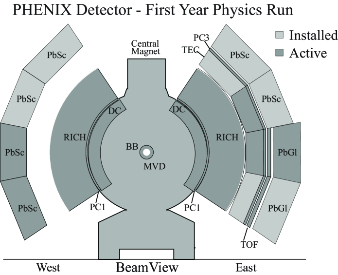
Figure 1: A cross-sectional view of the PHENIX detector, transverse to the beamline. Within the two central arm spectrometers the detectors that were instrumented and operational during the $\sqrt{s_{NN}}=130$ GeV run are shown.

II.1 CENTRAL ARM DETECTORS

The central arm spectrometers use a central magnet that produces an approximately axially symmetric field that focuses charged particles into the detector acceptance. The two central arms are labeled as East and West Arms. The East Arm contains the following subsystems used in this analysis: drift chamber (DC), pad chamber (PC), and a Time-of-Flight (TOF) wall. The PHENIX hadron acceptance using the TOF system in the East Arm is illustrated in Figure 2 where the transverse momentum is plotted as a function of the particle rapidity (the phase space) within the central arm acceptance subtending the polar angle $\theta$ from 70 to 110 degrees for pions, kaons, and protons. The vertical lines are the equivalent pseudorapidity edges, corresponding to $|\eta|<0.35$. More details are discussed elsewhere Mitchell et al. (2002).

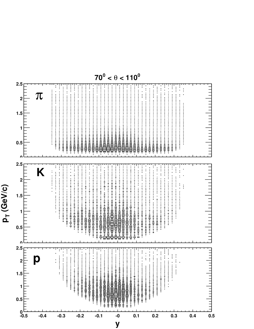
Figure 2: The central arm spectrometer acceptance in rapidity and transverse momentum for pions (top), kaons (middle), and protons (bottom).

II.1.1 TRACKING CHAMBERS

The charged particle tracking chambers include three layers of pad chambers and two drift chambers. The chambers are designed to operate in a high particle multiplicity environment.

The drift chambers are the first tracking detectors that charged particles encounter as they travel from the collision vertex through the central arms. Each is 1.8 m in width in the beam direction, subtends 90-degrees in azimuthal angle $\phi$, centered at a radius $R_{DC}=2.2$ m, and is filled with a 50-50 Argon-Ethane gas mixture. It consists of 40 planes of sense wires arranged in 80 drift cells placed cylindrically symmetric about the beamline. The wire planes are placed in an X-U-V configuration in the following order (moving outward radially): 12 X planes (X1), 4 U planes (U1), 4 V planes (V1), 12 X planes (X2), 4 U planes (U2), and 4 V planes (V2). The U and V planes are tilted by a small $\pm 5^{o}$ stereo angle to allow for full three-dimensional track reconstruction. The field wire design is such that the electron drift to each sense wire is only from one side, thus removing most left-right ambiguities everywhere except within 2 mm of the sense wire. The wires are divided electrically in the middle at the beamline center. The occupancy for a central RHIC Au+Au collision is about two hits per wire.

At the drift chamber location, the field of the central magnet is nearly zero, so the DC determines (nearly) straight-line track segments in the r-$\phi$ plane. Each track segment is intersected with a circle at $R_{DC}$, where it is characterized by two angles: the angular deflection in the main bend plane, and the azimuthal position in $\phi$. A combinatorial Hough transform technique (CHT) is used to identify track segments by searching for location maxima in this angular space/citehough. The DCs are calibrated with respect to the event collision time measurement (see Section  II.2). With this calibration, the single-wire resolution in the r-$\phi$ plane is 160 $\rm{\mu}$m. The single-track wire efficiency is  99% and the two-track resolution is better than 1.5 mm.

The drift chambers are used to measure the momentum of charged particles and the direction vector for charged particles traversing the spectrometer. The angular deflection is inversely proportional to the component of momentum in the bend plane only. Both the bend angle and the measured track points are used in the momentum reconstruction and track model, which uses a look-up table of the measured central magnet field grid. For this data set, the drift chamber momentum resolution is $\sigma_{p}/p=0.6\%\oplus 3.6\%p$, where the first term is multiple scattering up to the drift chambers and the second is the angular resolution of the detector.

In Run-1, there were three pad chambers in PHENIX. Each pad chamber measures a three-dimensional space point of a charged track. The pad chambers are pixel-based detectors with effective readout sizes of 8.45 mm along the beamline by 8.40 mm in the plane transverse to the beamline. The first pad chamber layer (PC1) is fixed to the outer edge radially of each drift chamber at a radial distance of 2.49 m, while the third layer (PC3) is positioned at 4.98 m from the beamline. Both arms include PC1 chambers, while only the East Arm is instrumented with PC3. The second layer (PC2) is located at an inner inscribed radius of 4.19 m in the West Arm and was not installed for Run-1.

The position resolution of PC1 is 1.6 mm along the beam axis and 2.3 mm in the plane transverse to the beam axis. The position resolutions of PC3 are 3.2 mm and 4.8 mm, respectively. The PC3 is used to reject background from albedo and non-vertex decay particles; however, only the PC1 is used for the results presented here. The PC1 is used in the global track reconstruction with the measured vertex position using the beamline detectors (see Section  II.2) to determine the polar angle of each charged track. Both PC1 and the beamline detectors provide z-coordinate information with a 1.89 mm resolution.

II.1.2 TIME OF FLIGHT

The Time-of-Flight detector (TOF) serves as the primary particle identification device for charged hadrons by the measurement of their arrival time at the TOF wall 5.1 m from the collision vertex. The TOF wall spans 30^∘ in azimuth in the East Arm. It consists of 10 panels of 96 scintillator slats each with an intrinsic timing resolution better than 100 ps. Each slat is oriented along the r-$\phi$ direction and provides timing as well as beam-axis position information for each particle hit recorded. The slats are viewed by two photomultiplier tubes, attached to either end of the scintillator. A $\pm\rm{2}\sigma$ $\pi$/K separation at momenta up to 2.0 GeV/c, and a $\pm\rm{2}\sigma$ ($\pi$+K)/proton separation up to 4.0 GeV/c can be achieved.

For each particle, the time, energy loss in the scintillator, and geometrical position are determined. The total time offset is calibrated slat by slat. A particle hit in the scintillator is defined by a measured pulse height which is also used to correct the time recorded at each end of the slat (slewing correction). After calibration, the average of the times at either end of the slat is the measured time for a particle. The azimuthal position is proportional to the time difference across the slat and the known velocity of light propagation in the scintillator (for Bicron BC404, this is 14 cm/ns). The slat position along the beamline determines the longitudinal coordinate position of the particle. The total time of flight is measured relative to the Beam-Beam counter initial time (see Section  II.2), the measured time in the Time-of-Flight detector, and a global time offset from the RHIC clock. Positive pions in the momentum range $1.4<p_{T}<1.8$ GeV/c are used to determine the TOF resolution. The timing calibration in this analysis results in a resolution of $\sigma=115$ ps.

Particle identification for charged hadrons is performed by combining the information from the tracking system with the timing information from the BBC and the TOF. Tracks at 1 GeV/c in momentum point to the TOF with a projected resolution $\sigma_{proj}$ of 5 mrad in azimuthal angle and 2 cm along the beam axis. Tracks that point to the TOF with less than 2.0 $\sigma_{proj}$ were selected. Figure 3 shows the resulting time-of-flight as a function of the reciprocal momentum in minimum-bias Au+Au collisions.

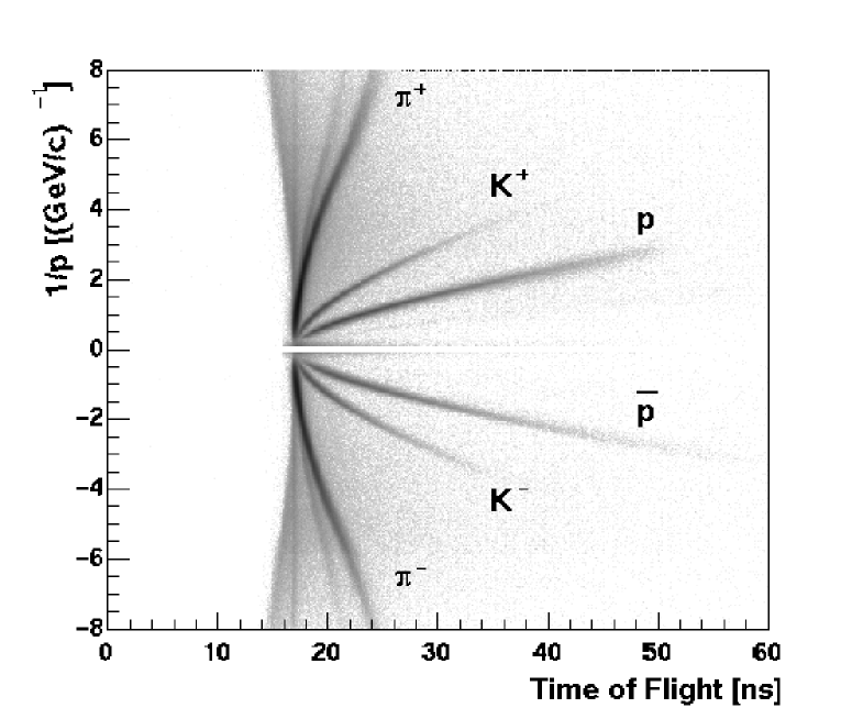
Figure 3: Scaled Time-of-Flight versus reciprocal momentum in minimum-bias Au+Au collisions at $\sqrt{s_{NN}}$ = 130 GeV. The distribution demonstrates the particle identification capability using the TOF for the Run-1 data taking period.

II.2 BEAMLINE DETECTORS

The beamline detectors determine the collision vertex position along the beam direction, and the trigger and timing information for each event. These detectors include the Zero Degree Calorimeters (ZDCs), the Beam-Beam Counters (BBC), and the Multiplicity Vertex Detector (MVD) and are positioned in PHENIX as shown in Figure 4.

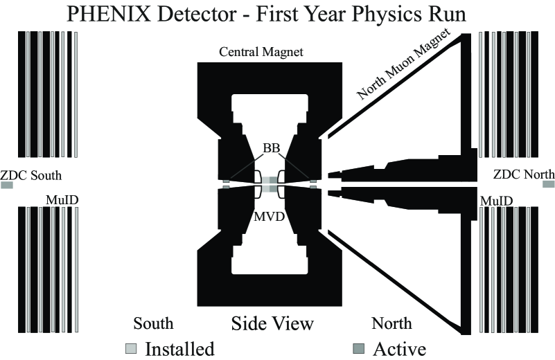
Figure 4: A side view of the PHENIX detector, parallel to the beamline. The beamline detectors determine the collision vertex position along the beam direction, and the trigger and timing information for each event.

The Zero Degree Calorimeters are small transverse area hadron calorimeters that are installed at each of the four RHIC experiments. They measure the fraction of the energy deposited by spectator neutrons from the collisions and serve as an event trigger for each RHIC experiment. The ZDCs measure the unbound neutrons in small forward cones ($\theta<$2 mrad) around each beam axis. Each ZDC is positioned 18 m up and downstream from the interaction point along the beam axis. A single ZDC consists of 3 modules each with a depth of 2 hadronic interaction lengths and read out by a single PMT. Both time and amplitude are digitized for each of the 3 PMTs as well as an analog sum of the PMTs for each ZDC. Adler et al. (2001b)

There are two Beam-Beam counters each positioned 1.4 m from the interaction point, just behind the central magnet poles along the beam axis (see Figure 4). The BBC consists of two identical sets of counters installed on both sides of the interaction point along the beam. Each counter consists of 64 Cherenkov telescopes, arranged radially about the collision axis and situated north and south of the MVD. The BBCs measure the fast secondary particles produced in each collision at forward angles, with $3.0\leq\eta\leq 3.9$, and full azimuthal coverage.

For both the ZDC and the BBC, the time and vertex position are determined using the measured time difference between the north and the south detectors and the known distance between the two detectors. The start time ($T_{0}$) and the vertex position along the beam axis ($Z_{vertex}$) are calculated as $T_{0}=(T_{1}+T_{2})/2$ and $Z_{vertex}=(T_{1}-T_{2})/2c$, where $T_{1}$ and $T_{2}$ are the average timing of particles in each counter and $c$ is the speed of light. With an intrinsic timing resolution of 150 ps, the ZDC vertex is measured to within 3 cm. In Run-1, the BBC timing resolution of 70 ps results in a vertex position resolution of 1.5 cm.

Event centrality is determined using a correlation measurement between neutral energy deposited in the ZDCs and fast particles recorded in the BBCs as shown in Figure 5. The spectator nucleons are unaffected by the interaction and travel at their initial momentum from each respective ion. The number of neutrons measured by the ZDC is proportional to the number of spectators, while the BBC signal increases with the number of participants.

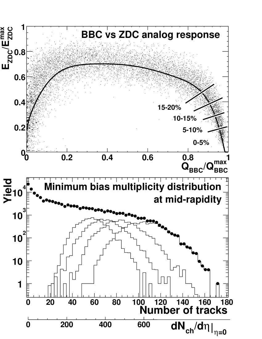
Figure 5: The event centrality (upper plot) is determined using a correlation measurement of the fraction of neutron energy recorded in the ZDCs (vertical scale) and the fractional charge measured in the BBCs (horizontal scale). The equivalent track multiplicity in each centrality selection is shown in the lower plot.

III DATA REDUCTION AND ANALYSIS

III.1 DATA REDUCTION

The PHENIX Level-1 trigger selected events with hits coincident in both the ZDC and BBC detectors, and in time with the RHIC clock. A total of 5M events were recorded at $\sqrt{s_{NN}}=$ 130 GeV in the ZDCs Zajc (2002). The collision position along the beam direction was required to be within $\pm$ 30 cm of the center of PHENIX, using the collision vertex reconstructed by the BBC.

The trigger on both BBC and both ZDC counters includes $92\pm 4\%$ of the total inelastic cross section ($6.8\pm 0.4$ barns). A Monte Carlo Glauber model Glauber and Natthiae (1970) is used with a simulation of the BBC and ZDC responses to determine the number of nucleons participating in the collisions for the minimum bias events. The Woods-Saxon parameters determined from electron scattering experiments are: radius $=6.38\pm 0.06$ fm, diffusivity $=0.54\pm 0.01$ fm Hahn et al. (1956), and the nucleon-nucleon inelastic cross-section, $\sigma^{inel}_{N+N}=40\pm 3$ mb. An additional systematic uncertainty enters the radius parameter since the radial distribution of neutrons in large nuclei should be larger than for protons and is not well determined Pollack et al. (1992).

The centrality selections used in this paper are 0-5%, 5-15%, 15-30%, 30-60%, and 60-92% of the total geometrical cross section, where 0-5% corresponds to the most central collisions.

Only tracks which are reconstructed in all three dimensions are included in the spectra. These tracks are then matched within 2$\sigma_{proj}$ to the measured positions in the TOF detector. For each TOF hit, the time, position, and energy loss are measured in the TOF detector. The widths of residual distance distributions between projected tracks and TOF hit positions, $\sigma_{proj}$, increase at lower momentum due to multiple scattering. Therefore, a momentum-dependent hit association criterion was defined.

Finally, a requirement on energy loss in the TOF is applied to each track to exclude false hits by requiring the energy deposit of at least minimum ionizing particle energy. A $\beta$-dependent energy loss cut whose form is a parameterization of the Bethe-Bloch formulaGroom (1998) is used, where

$$dE/dx\approx\beta^{-5/3}$$ (1)

and $\beta=L/ct$, where $L$ is the pathlength of the particle’s trajectory from the BBC vertex to the TOF detector, t is the particle’s time-of-flight, and c is the speed of light. The approximate Bethe-Bloch formula is scaled by a factor to fall below the data and thereby serve as a cut. The resulting equation is $\Delta E=A\beta^{-5/3}$ where A is a scaling factor equal to $1.6$ MeV. The energy loss cut reduces low momentum background under the kaon and proton mass peaks. The fraction of tracks excluded after the energy loss cut is less than $5.5\%$.

The measured momentum ($p$), pathlength ($L$), and time of flight ($t$) in the spectrometer are used to calculate the particle mass, which is used for particle identification:

$$m^{2}=\frac{p^{2}}{c^{2}}\left[{{\left(\frac{1}{\beta}\right)}^{2}-1}\right].$$ (2)

The width of the peaks in the mass-squared distribution depend on both the momentum and time-of-flight resolutions. An analytic form for the width of $m^{2}$ as a function of momentum resolution $\sigma_{p}$ and time of flight resolution is determined using Equation 2. The error in the particle’s pathlength L results in an effective time width that is included with the TOF resolution, $\sigma_{T}$,

$$\sigma^{2}_{m^{2}}=4m^{4}{\frac{\sigma_{p}}{p}}^{2}+4p^{4}\frac{1}{\beta^{2}}{\frac{\sigma_{T}}{t}}^{2}.$$ (3)

The momentum resolution of the drift chambers is expressed in the following form

$$\sigma_{p}^{2}={\left(C_{1}p\frac{1}{\beta}\right)}^{2}+{\left(C_{2}p^{2}\right)}^{2},$$ (4)

$$C_{1}=\frac{\delta\phi_{ms}}{K_{1}},$$ (5)

$$C_{2}=\frac{\delta\phi_{\alpha}}{K_{1}},$$ (6)

where $C_{1}$ and $C_{2}$ are the multiple scattering and angular resolution terms, respectively. The units of $\delta\phi_{ms}$ are mrad GeV/c. The constant $K_{1}$ is the momentum kick on the particle from the magnetic field and is equal to $87.3$ mrad GeV/c. The constant $C_{1}$ is the width in $\phi$ due to the multiple scattering (ms) of a charged particle with materials of the spectrometer up to the drift chambers. The $C_{2}$ term is the angular resolution of the bend angle ($\alpha$), which is the angular deflection in $\phi$ of the track segment relative to the radius to the collision vertex.

Equation 4 is used in Equation 3 with $\beta=p/\sqrt{p^{2}+m^{2}_{0}}$, where $m_{0}$ is the mass centroid of the particle’s mass-squared distribution. The mass centroid is close to the rest mass of the particle; however due to residual misalignments and timing calibration, the centroid of the distribution is a fit parameter in order to avoid cutting into the distribution. The $m^{2}$ width for each particle is written as follows:

$$\sigma^{2}_{m^{2}}=$$

$$C_{1}^{2}\cdot 4m^{4}(1+\frac{m^{2}_{0}}{p^{2}})+C_{2}^{2}\cdot 4m^{4}_{0}p^{2}+C_{3}^{2}\cdot(4p^{2}(m_{0}^{2}+p^{2}))$$

where the coefficient $C_{3}$ is related to the combined TOF,

$$C_{3}=\frac{\sigma_{T}c}{L},$$ (8)

and pathlength contributions to the time width, $\sigma_{T}$ in Equation  8. From the measured drift chamber momentum resolution, $C_{1}=0.006$ and $C_{2}=0.036$ c/GeV. While the TOF resolution is 115$\pm$5 ps, the pathlength uncertainty introduces a width of $\approx$ 20-40 ps, so 145 ps is used for $\sigma_{T}$ in $C_{3}$.

The pions, kaons, and protons are identified using the measured peak centroids of the $m^{2}$ distribution and selecting $2\sigma$ bands; shown as shaded regions in Figure 6 for two different momentum slices. The 2$\sigma$ bands for pions and kaons do not overlap up to $p_{T}=$2 GeV/c. The protons are identified up to $p_{T}=$ 4 GeV/c. By studying variations in the $m^{2}$ centroid and width before the particle identification cut is applied, the uncertainty in the particle identification is estimated to be 5$\%$ for all particles.

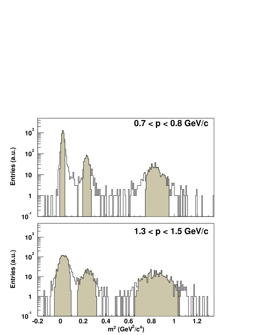
Figure 6: The mass-squared distributions of positive pions, kaons, and protons for two different momentum slices. The momentum slice $\rm{0.7}<p<\rm{0.8}$ GeV/c is the upper panel and $\rm{1.3}<p<\rm{1.5}$ GeV/c is the lower panel. The shaded regions correspond to the 2$\sigma$ particle identification bands based on the calculated mass-squared width, the measured mass-squared centroids, and the known detector resolutions.

Kaons are depleted by decays in flight and geometrical acceptance. For the low momentum protons, energy loss and geometrical acceptance cause a drop in the raw yield for $p_{T}<\rm{0.5}$ GeV/c, as seen in Figure 2.

The remaining background contribution was determined by reflecting the track about the midpoint of PHENIX along the beamline and repeating the association and PID cuts used in the TOF detector. This random background was evaluated separately for each particle type. The background contribution is $\approx$ 30% for the kaon spectra at $\rm{0.2}<p_{T}<\rm{0.4}$ GeV/c and defines the low $p_{T}$ limit in the spectra. The background is $<\rm{5}\%$ in all other cases, and negligible above 0.8 GeV/c in the measured momentum range in this analysis. The background was not subtracted but is instead treated as a systematic uncertainty. This uncertainty is 2, 5, and 3$\%$ for pions, kaons, and protons, respectively, at $p_{T}<\rm{0.6}$ GeV/c and is negligible at higher momenta.

III.2 ANALYSIS

The raw spectra include inefficiencies from detector acceptance, resolution, particle decays in flight and track reconstruction. The baseline efficiencies are determined by simulating and reconstructing single hadrons. Multiplicity dependent effects are then evaluated by embedding simulated single hadrons into real events and calculating the degradation of the reconstruction efficiency.

III.2.1 CORRECTIONS: ACCEPTANCE, DECAYS IN FLIGHT, AND DETECTOR RESPONSE

The corrections for the finite detector aperture, pion and kaon decays in flight, and the detector response are determined using single particles in the the GEANT Brun et al. (1978) simulation of the detector. All details of each detector are modeled, including dead channels in the drift chambers, pad chambers, and Time-of-Flight detector. All physics processes are automatically taken into account, resulting in corrections for multiple scattering, anti-proton annihilation, pion and kaon decays in flight, finite geometrical acceptance of the detector, and momentum resolution, which affects the spectral shape above 2.5 GeV/c.

The drift chamber simulated response is tuned to describe the response of the real drift chambers on the single-wire level. This is done using a simple geometrical model of the drift chamber and the straight-line trajectories of particles from the zero-field data. This simple model of the drift cell in the drift chamber is sufficient to describe the observed drift distance distribution, the pulse width, the single wire efficiency, and the detector resolution. The TOF response is simulated by smearing the true time of flight using a Gaussian distribution with a width as measured in the data.

Figure 7 shows the momentum dependence of the residual distance between projected tracks and TOF hits for the real (solid line) and simulated (dashed) events. These residuals are parameterized in the azimuthal angle $\phi$ and the beamline direction $z$, separately for data and simulation. For each case, tracks that fall outside 2$\sigma$ of the parameterized width are rejected, thus allowing use of the Monte Carlo to evaluate the correction for the 2$\sigma$ match requirement for real tracks.

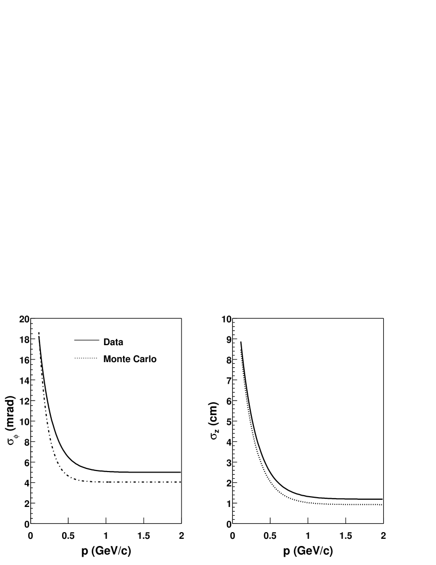
Figure 7: Comparison of the momentum-dependent residuals of DC tracks matched to TOF hits in azimuthal angle $\phi$ (left) and z (right) between data (solid) and simulation (dashed).

A fiducial cut is made in both the simulation and in the data to ensure the same fiducial volume. The systematic uncertainty in the acceptance correction is approximately 5$\%$.

The simulated distributions are generated uniformly in $p_{T}$, $\phi$, and $y$. For each hadron, sufficient Monte Carlo events are generated to obtain the correction factor for every measured $p_{T}$ bin. The statistical errors from the correction factors were smaller than those in the data and both are added in quadrature.

The distribution of the number of particles generated in each $p_{T}$ slice, dN/d$p_{T}$, is the “ideal” input distribution without detector and reconstruction effects. This distribution is normalized to 2$\pi$ and 1 unit of rapidity. After detector response and track reconstruction, the output distribution is the number of particles found in each $p_{T}$ slice. The final corrections are determined after an iterative weighting procedure. First, the flat input and output distributions are weighted by exponential functions for all particles using an inverse slope of 300 MeV. The ratio of input to output distributions is determined as a function of momentum. In each $p_{T}$ slice, the corresponding ratio is applied to the data. The corrected data are next fitted with exponentials for kaons and protons (see Equation 11), and a power-law for the pions (see Equation 9). The original flat input and output distributions are weighted by these resulting functions. The procedure is repeated until the functions remain constant in their parameters. The weighted input and output distributions are divided to produce acceptance correction factors. The corrections are larger for kaons due to the decays in flight. The statistical error in determination of the correction factor is added in quadrature to the statistical error in the data.

III.2.2 HIGH TRACK-DENSITY EFFICIENCY CORRECTION

A final multiplicity dependent correction is determined using simulated single-particles embedded into real events. This correction depends on both the quality of the track reconstruction in a high multiplicity environment and the type of particle measured.

Depending on the centrality of the event, the correction factor is determined for each particle in the raw transverse momentum distribution and is applied as a weight. The final efficiency corrections are shown in Figure 8, where the correction for pions is shown as solid circles and for (anti)protons as open circles. The horizontal axis ranges from the most central to the most peripheral events in increments of 5%. The systematic uncertainty in the multiplicity efficiency correction is 9%.

The difference between pions (solid) and (anti)protons (open) is due to the different TOF efficiencies for each particle (protons are slower than pions). In a small fraction of cases two particles may hit the same TOF slat at different times, and the slower particle is assigned an incorrect time. The particle will then fall outside the particle identification cuts. This effect depends on the type of particle.

For each particle, two curves are shown, representing the DC tracking inefficiency for two types of tracks: fully reconstructed and partially reconstructed tracks. Fully reconstructed tracks include X1 and X2 sections. In a high track-density environment, tracks may be partially reconstructed or hits may be incorrectly associated. There are two cases when this incorrect hit association occurs. In the first case, the direction vector in the azimuth prevents the track from pointing properly to the PC1 detector, and the correct hit cannot be associated. In the second case, the track is reconstructed properly, but there are two possible PC1 points. If no UV hits are found, then the wrong PC1 point can be associated to the track and the track’s beamline coordinate is mis-reconstructed. In both of these cases, the track fails the matching criteria in the TOF detector and is lost.

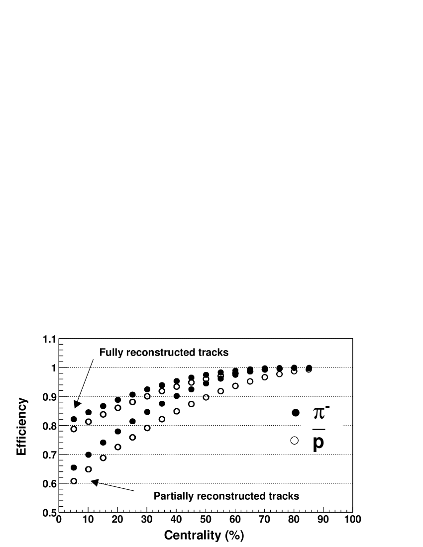
Figure 8: The multiplicity dependent efficiency correction for pions (solid) and (anti)protons (open) for two types of tracks. The upper set of points correspond to fully reconstructed tracks in the drift chambers; while the lower set of points correspond to partially reconstructed tracks in the drift chambers.

III.2.3 DETERMINING THE YIELD AND MEAN $p_{T}$

The dN/dy and $\langle p_{T}\rangle$ are determined using the data in the measured region and an extrapolation to the unmeasured region after integrating a functional form fit to the data. A function describing the spectral shape is fit to the data, with varying $p_{T}$ ranges to control systematic uncertainties in the fit parameters. The fitted shape is extrapolated, integrated over the unmeasured range, and then combined with the measured data to get the full yield. Two different functions are used to estimate upper and lower bounds for each spectrum. The average between the upper and lower bounds is used for dN/dy and $\langle p_{T}\rangle$. The statistical error is determined from the data, and the systematic uncertainty is taken as 1/2 the difference between the upper and lower bounds.

For pions, a power-law in $p_{T}$ (Equation  9) and an exponential in $m_{T}(=\sqrt{p^{2}_{T}+m^{2}_{0}})$ (Equation  10) are fit to the data. For kaons and (anti)protons, two exponentials, one in $p_{T}$ (Equation  11) and the other in $m_{T}$ are used. The $p_{T}$ exponential provides an upper limit for the extrapolated yield, which is most important for the (anti)protons. The power-law function has three parameters labeled $A$, $p_{0}$, and $n$ in Equation  9. The exponentials have two parameters, $A$ and $T$.

$$\frac{d^{2}N}{2\pi p_{T}dp_{T}dy}=A\left(\frac{p_{0}}{p_{0}+p_{T}}\right)^{n}$$ (9)

$$\frac{d^{2}N}{2\pi m_{T}dm_{T}dy}=Ae^{-m_{T}/T}$$ (10)

$$\frac{d^{2}N}{2\pi p_{T}dp_{T}dy}=Ae^{-p_{T}/T}$$ (11)

III.3 SYSTEMATIC UNCERTAINTIES

In Table  1, the sources of systematic uncertainties in both $\langle p_{T}\rangle$ and dN/dy are tabulated. The sources of uncertainty include the extrapolation in $p_{T}$, the background, and the Monte Carlo corrections and cuts. The uncertainty in the Monte Carlo corrections is 11% and includes: the multiplicity efficiency correction of 9%, the particle identification cut of 5%, and the fiducial cuts of 5%. The uncertainties in the correction functions are added in quadrature to the statistical error in the data. Background is only relevant for $p_{T}<0.6$ GeV/c in the spectra.

The total systematic uncertainty in the $\langle p_{T}\rangle$ depends on the extrapolation and background uncertainties; the uncertainties are 7$\%$, 10$\%$, and 8$\%$ for pions, kaons, and protons, respectively. The overall uncertainty on dN/dy includes the uncertainties on $\langle p_{T}\rangle$ in addition to the uncertainties from the corrections and cuts; the uncertainties are 13$\%$, 15$\%$, and 14$\%$ for pions, kaons, and protons, respectively Burward-Hoy (2001).

The hadron yields and $\langle p_{T}\rangle$ values include an additional uncertainty arising from the fitting function used for extrapolation to the unmeasured region at low and high $p_{T}$. The magnitude of the extrapolation is $30\pm 6\%$ of the spectrum for pions, $40\pm 8\%$ for kaons, and $25\pm 7.5\%$ for protons Burward-Hoy (2001). The systematic uncertainty quoted here is taken as 1/2 the difference between the results from the two different functional forms.

Table 1: The sources of systematic uncertainties in $\langle p_{T}\rangle$ and dN/dy.

	$\pi$ (%)	K (%)	(anti)p (%)
Extrapolation	6	8	7.5
Background ($p_{T}<0.6$ GeV/c)	2	5	3
$\langle p_{T}\rangle$ total	7	10	8
Corrections and cuts	11	11	11
dN/dy total	13	15	14

The momentum scale is known to better than 2%, and the momentum resolution affects the spectra shape, primarily for protons, above 2.5 GeV/c. The momentum resolution is corrected by the Monte Carlo. As other sources of uncertainty on the number of particles at any given momentum are much larger, momentum resolution effects are neglected in determining the overall systematic uncertainty from the data reduction.

IV RESULTS

IV.1 TRANSVERSE MOMENTUM DISTRIBUTIONS

The invariant yields as a function of $p_{T}$ for identified hadrons are shown in Figure 9, while Figure 10 provides the centrality dependence of the spectra. The spectra are tabulated in Appendix B. The $\pi^{\pm}$, $K^{\pm}$, p, and $\overline{p}$ invariant yields for the most central, mid-central, and the most peripheral collisions, were reported previously Adcox et al. (2002b). Pion and (anti-)proton invariant yields are comparable for $p_{T}>$1 GeV in the most central collisions.

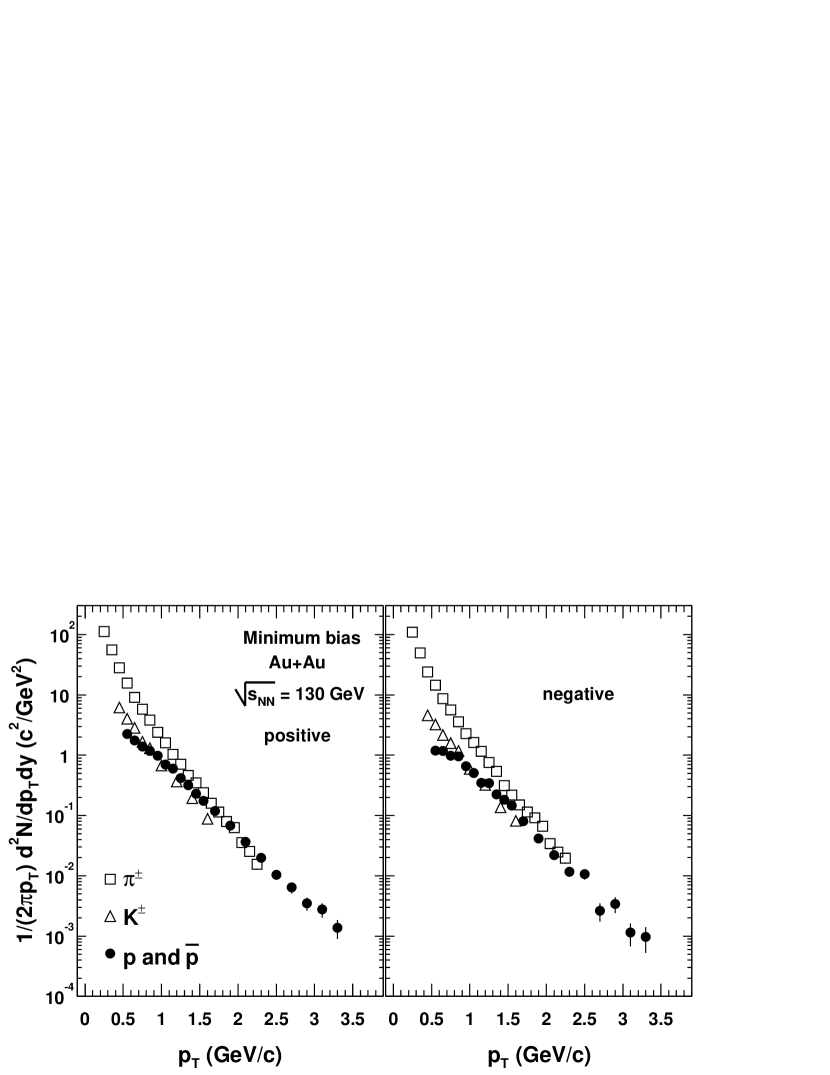
Figure 9: The spectra of positive particles (left) and negative (right) in minimum-bias collisions from Au+Au collisions at $\sqrt{s_{NN}}=$130 GeV. The errors include both statistical and systematic errors from the corrections.

Figure 10: The hadron spectra for five centralities from the most central 0-5% to the most peripheral 60-92% at $\sqrt{s_{NN}}=$ 130 GeV. Errors include both the statistical and point-by-point error in the corrections added in quadrature.

As can be seen already from Figure 10 all the spectra seem to be exponential; however, upon closer inspection, small deviations from an exponential form are apparent for the more peripheral collisions. The spectrum in the most peripheral collisions is noticeably power-law-like when compared to the more exponential-like spectrum in central collisions. This is especially apparent for the pions. The effect can be seen more clearly in the ratio of the spectra for a given particle species in two different centrality classes. Such ratios are shown in Figure 11 for the 5% central and the most peripheral positive spectra (60-92% centrality). The ratios for protons and antiprotons as well as for $\pi^{+}$ have a maximum at intermediate $p_{T}$ and are lower both at low and high $p_{T}$. The kaon shape change is not very significant, given the current statistics.

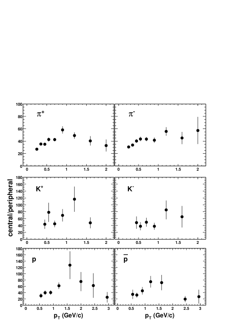
Figure 11: The ratio of the most central to the most peripheral yields as a function of $p_{T}$ for pions (top), kaons (middle) and (anti)protons (bottom).

The change in slope at low-$p_{T}$ in central collisions compared to peripheral is consistent with a more substantial hydrodynamic, pressure-driven transverse flow existing in central collisions, since the increased boost would tend to deplete particles at the lowest $p_{T}$ (see Section IV.3). This is observed at lower energies at the CERN SPS Albrecht et al. (1998); Aggarwal et al. (2002). It is in contrast to results obtained at the ISR Faessler (1984) for p+p collisions at $\sqrt{s}=$ 63 GeV, where a shallow maximum or minimum exists at low $p_{T}$ (in the range $0.3-0.6$ GeV/c).

IV.1.1 FEED-DOWN CONTRIBUTION TO p AND $\overline{p}$ FROM INCLUSIVE $\Lambda$ and $\overline{\Lambda}$

Inclusive $\Lambda$ and $\overline{\Lambda}$ transverse momentum distributions have been measured in the west arm of the PHENIX spectrometer using the tracking detectors (DC, PC1) and a lead-scintillator electromagnetic calorimeter (EMCal) Adcox et al. (2002c). The invariant mass is reconstructed from the weak decays $\Lambda\rightarrow p+\pi^{-}$ and $\overline{\Lambda}\rightarrow\overline{p}+\pi^{+}$.

The tracks from the tracking detectors are required to fall within 3$\sigma$ of EMCal measured space-points. The EMCal timing resolution of the daughter particles is $\approx$ 700 ps. Using the DC momentum and the EMCal time-of-flight, the particle mass is calculated, and protons, antiprotons, and pions are identified using 2$\sigma$ momentum-dependent mass-squared cuts. A clean particle separation is obtained using an upper momentum cut of 0.6 GeV/c and 1.4 GeV/c for pions and protons, respectively. The momentum is determined assuming the primary decay vertex is positioned at the event vertex and results in a momentum shift of 1-2% based on a Monte Carlo study.

Using all combinations of pions and protons, the invariant mass is determined. The mass distribution shows a $\Lambda$ peak on top of a random combinatorial background, which is determined by combining protons and pions from different collisions with the same centrality. A signal-to-background ratio of 1/2 is obtained after applying a decay kinematic cut on the daughter particles. Fitting a Gaussian function to the mass distribution in the range $\rm{1.05}<m_{\rm{p\pi}}<\rm{1.20}~{}GeV/c^{2}$, 12000 $\Lambda$ and 9000 $\overline{\Lambda}$ are observed, with mass resolution $\delta m/m\approx$ 2%. The reconstructed $\Lambda$ and $\overline{\Lambda}$ spectra are corrected for the acceptance, pion decay-in-flight, momentum resolution, and reconstruction efficiency Adcox et al. (2002c). The systematic uncertainty on the $p_{T}$ spectra is 13% from the corrections and 3% from the combinatorial background subtraction. The feed-down contributions from heavier hyperons $\Sigma^{0}$ and $\Omega$ are not measured but are estimated to be $<$ 5%.

In Figure 12, the transverse momentum spectra of inclusive protons (left) and antiprotons (right) are shown with the inclusive $\Lambda$ and $\overline{\Lambda}$ transverse momentum distributions. The solid points are the (anti)proton spectra after the feed-down correction from $\Lambda$ and $\overline{\Lambda}$ weak decays. From here forward, the data that are presented and discussed are not corrected for this feed-down effect; inclusive p and $\overline{p}$ yields are given. More details on the $\Lambda$ and $\overline{\Lambda}$ measurement are included in Adcox et al. (2002c).

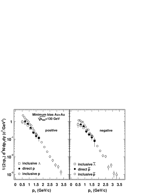
Figure 12: For minimum-bias collisions, the inclusive $\Lambda$, inclusive p, and direct p transverse momentum distributions are plotted together in the left panel. The equivalent comparison for inclusive $\overline{\Lambda}$, $\overline{p}$, and direct $\overline{p}$ transverse momentum distributions is in the right panel.

IV.2 YIELD AND $\langle p_{T}\rangle$

The yield, dN/dy, and the average transverse momentum, $\langle p_{T}\rangle$, are determined for each particle as described in the preceding section and have been previously published in Adcox et al. (2002b). For each centrality, the rapidity density dN/dy and average transverse momentum $\langle p_{T}\rangle$ are tabulated in Tables 2 and  3, respectively.

The $N_{part}$ and $N_{coll}$ in each centrality selection are determined using a Glauber-model calculation in Adcox et al. (2001b). The resulting values of $N_{part}$ and $N_{coll}$ are also tabulated in Table 2. (See Appendix  A for more detail). The errors on $N_{part}$ and $N_{coll}$ include the uncertainties in the model parameters as well as in the fraction of the total geometrical cross section ($92\%\pm 4\%$) seen by the interaction trigger. The error due to model uncertainties is 2% Adcox et al. (2001b). An additional 3.5% error results from time dependencies in the centrality selection over the large data sample.

Table 2: The dN/dy at midrapidity for hadrons produced at midrapidity in each centrality class. The errors are statistical only. The systematic errors are 13%, 15% and 14% for pions, kaons, and (anti)protons, respectively. The $N_{part}$ and $N_{coll}$ in each centrality selection are from a Glauber-model calculation in Adcox et al. (2001b), also shown with systematic errors based on a 92$\pm$4% coverage.

	0-5%	5-15%	15-30%	30-60%	60-92%
$N_{part}$	$347.7\pm 10$	$271.3\pm 8.4$	$180.2\pm 6.6$	$78.5\pm 4.6$	$14.3\pm 3.3$
$N_{coll}$	1008.8	712.2	405.5	131.5	14.2
$\pi^{+}$	$276\pm 3$	$216\pm 2$	$141\pm 1.5$	$57.0\pm 0.6$	$9.6\pm 0.2$
$\pi^{-}$	$270\pm 3.5$	$200\pm 2.2$	$129\pm 1.4$	$53.3\pm 0.6$	$8.6\pm 0.2$
$K^{+}$	$46.7\pm 1.5$	$35\pm 1.3$	$22.2\pm 0.8$	$8.3\pm 0.3$	$0.97\pm 0.11$
$K^{-}$	$40.5\pm 2.3$	$30.4\pm 1.4$	$15.5\pm 0.7$	$6.2\pm 0.3$	$0.98\pm 0.1$
$p$	$28.7\pm 0.9$	$21.6\pm 0.6$	$13.2\pm 0.4$	$5.0\pm 0.2$	$0.73\pm 0.06$
$\overline{p}$	$20.1\pm 1.0$	$13.8\pm 0.6$	$9.2\pm 0.4$	$3.6\pm 0.1$	$0.47\pm 0.05$

Table 3: The $\langle p_{T}\rangle$ in MeV/c for hadrons produced at midrapidity in each centrality class. The errors are statistical only. The systematic uncertainties are 7%, 10%, and 8% for pions, kaons, and (anti)protons, respectively.

	0-5%	5-15%	15-30%	30-60%	60-92%
$\pi^{+}$	$390\pm 10$	$380\pm 10$	$380\pm 20$	$360\pm 10$	$310\pm 30$
$\pi^{-}$	$380\pm 20$	$390\pm 10$	$380\pm 10$	$370\pm 20$	$320\pm 20$
$K^{+}$	$560\pm 40$	$580\pm 40$	$570\pm 40$	$550\pm 40$	$470\pm 90$
$K^{-}$	$570\pm 50$	$590\pm 40$	$610\pm 40$	$550\pm 50$	$460\pm 90$
$p$	$880\pm 40$	$870\pm 30$	$850\pm 30$	$800\pm 30$	$710\pm 80$
$\overline{p}$	$900\pm 50$	$890\pm 40$	$840\pm 40$	$820\pm 40$	$800\pm 100$

Pions dominate the charged particle multiplicity, but a large number of kaons and (anti)protons are produced. The inclusive yield of antiprotons is nearly comparable to that of protons. In the most central Au+Au collisions, the particle density at midrapidity (dN/dy) is $\approx$ 20 for antiprotons and 28 for protons, not corrected for feed-down from strange baryons.

The average transverse momenta increase with particle mass and with decreasing impact parameter. The mean transverse momentum increases with the number of participant nucleons by 20$\pm$5% for pions and protons, as shown in Figure 13. The $\langle p_{T}\rangle$ of particles produced in $p+p$ and $p\overline{p}$ collisions, extrapolated to RHIC energies, are consistent with the most peripheral pion and kaon data; however, the $\langle p_{T}\rangle$ of protons produced in Au+Au collisions is significantly higher. This dependence on the number of participant nucleons may be due to radial expansion.

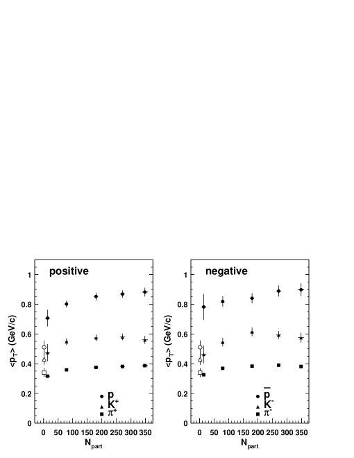
Figure 13: The integrated mean $p_{T}$ for pions, kaons, and (anti)protons produced in the five different classes of event centrality Adcox et al. (2002b). The error bars are statistical only. The systematic uncertainties are 7%, 10%, and 8% for pions, kaons, and (anti)protons, respectively. The open points are equivalent average transverse momenta from $pp$ and $p\overline{p}$ data, interpolated to $\sqrt{s}$=130 GeV.

IV.3 TRANSVERSE MASS DISTRIBUTIONS

Production of hadrons from a thermal source would make transverse mass the natural variable for analysis. Therefore we extract inverse slopes from the transverse mass distributions by separately fitting a thermal distribution to each particle species. The Boltzmann distribution is given in equation 12.

$$\frac{d^{2}N}{2\pi m_{T}dm_{T}dy}=Am_{T}e^{-m_{T}/T_{eff}},$$ (12)

We use a simple exponential, however, with no powers of $m_{T}$ in the prefactor, as shown in equation 10. This simplification is acceptable as the difference in the inverse slope is found to be less than 2%. The simple $m_{T}$ exponential was also used in an equivalent analysis in Reference Bearden et al. (1997). The inverse slope, $T_{eff}$, can be compared to other experiments, provided the same momentum range of the spectrum is used for fitting.

If the system develops collective motion, particles experience a velocity boost from this motion, resulting in an additional transverse kinetic energy component. This motivates use of the transverse kinetic energy, i.e. transverse mass minus the particle rest mass, for plotting data. Figure 14 shows the transverse kinetic energy distributions (i.e. transverse mass minus the particle rest mass) for all positive particles (left) and negative particles (right). Pions are in the top panel, kaons in the middle panel, and (anti)protons in the bottom panel, with different symbols indicating different centrality bins. The solid lines are $m_{T}$ exponential fits in the range $(m_{T}-m_{0})<1$ GeV for all particle species while the dashed lines are the extrapolated fits. The pion spectra follow an exponential for $0.38<(m_{T}-m_{0})<1.0$ GeV while the kaons and protons appear exponential over the entire measured $m_{T}$ range. The same is true for the negative particles in the right panel; however, the antiprotons have more curvature for $(m_{T}-m_{0})<0.5$ GeV. We extract $T_{eff}$ by fitting exponentials of the form Equation  10 to the transverse mass spectra in the range $(m_{T}-m_{0})<$1 GeV.

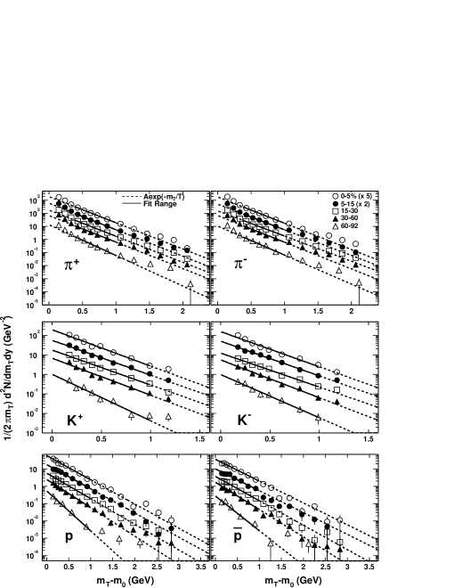
Figure 14: Transverse mass distributions of pions (top), kaons (middle), and (anti)protons (bottom) in events with different centralities. Positive particle distributions are on the left and negative particle distributions are on the right. The solid lines are $m_{T}$ exponential fits in the range $(m_{T}-m_{0})<1$ GeV for all particle species while the dashed lines are the extrapolated fits.

This range is chosen common for all particle species and minimizes contributions from hard processes. Caution must be taken when comparing $T_{eff}$ values as the local slope of the transverse mass spectra varies somewhat over $m_{T}$ for pions and antiprotons even within this fit range. The resulting values of $T_{eff}$ for all particles and centralities are tabulated in Table 4 in units of MeV. The inverse slopes increase and then saturate for more central collisions for all particles except antiprotons. The fact that the inverse slope is different for mesons and baryons and for central and peripheral events is consistent with the mean $p_{T}$ trends discussed above.

Table 4: The resulting inverse slopes in MeV after fitting an $m_{T}$ exponential to the spectra in the range $m_{T}-m_{0}<$1 GeV in each event centrality classes. The pion resonance region is excluded in the fits. The equivalent $p_{T}$ fit range for each particle is shown accordingly. The errors are statistical only.

	0-5%	5-15%	15-30%	30-60%	60-92%
$\pi^{+}$ in $0.5<p_{T}<1.05$ GeV/c	216.8 $\pm$ 5.7	214.3 $\pm$ 4.6	217.4 $\pm$ 4.7	214.4 $\pm$ 5.2	176.9 $\pm$ 9.5
$\pi^{-}$ in $0.5<p_{T}<1.05$ GeV/c	215.8 $\pm$ 6.5	221.2 $\pm$ 5.6	225.3 $\pm$ 5.8	212.8 $\pm$ 5.7	215.8 $\pm$ 16.8
$K^{+}$ in $0.45<p_{T}<1.35$ GeV/c	233.2 $\pm$ 10.8	243.6 $\pm$ 9.8	242.4 $\pm$ 9.2	228.7 $\pm$ 10.2	182.3 $\pm$ 19.0
$K^{-}$ in $0.45<p_{T}<1.35$ GeV/c	241.1 $\pm$ 15.8	244.5 $\pm$ 10.2	250.0 $\pm$ 12.3	224.2 $\pm$ 11.1	196.4 $\pm$ 22.3
$p$ in $0.55<p_{T}<1.85$ GeV/c	310.8 $\pm$ 14.8	311.0 $\pm$ 12.3	293.8 $\pm$ 11.4	265.3 $\pm$ 10.9	200.9 $\pm$ 14.8
$\overline{p}$ in $0.55<p_{T}<1.85$ GeV/c	344.2 $\pm$ 25.3	344.0 $\pm$ 20.9	307.6 $\pm$ 17.1	275.1 $\pm$ 14.0	217.0 $\pm$ 28.3

We compare to published inverse slopes of transverse mass distributions at midrapidity from $m_{T}$ exponential fits in the region $(m_{T}-m_{0})<1.2$ GeV, listed in Table 5. The comparison includes NA44 Bearden et al. (1997); Boggild et al. (1999); Bearden et al. (1998, 1996) and WA97  Andersen et al. (1999); Antinori et al. (1998) at the SPS at $\sqrt{s_{NN}}=17$ GeV; and, at $\sqrt{s_{NN}}=23$ GeV at the ISR, Alper et al. Alper et al. (1975a) and Guettler et al. Guettler et al. (1976). These data are chosen as they match the ($m_{T}-m_{0}$) range used in fitting our data. For pions, the low-$p_{T}$ region of ($m_{T}-m_{0})<0.3$ GeV, populated by decay of baryonic resonances, is systematically excluded from the fits. The effective temperatures are given in Table 5 with the references noted accordingly.

Table 5: Inverse slope parameters (in MeV) of hadrons for p+p, p+nucleus, and central S+S, S+Pb, and Pb+Pb colliding systems at CERN energies. Pb+Pb is at $\sqrt{s_{NN}}=17$ GeV, and the other systems at 23 GeV. The errors are statistical and systematic, respectively.

Hadron	Pb+Pb	S+Pb	S+S	p+Pb	p+S	p+Be	p+p
$\pi^{+}$	156$\pm$6$\pm$23	165$\pm$9$\pm$10	148$\pm$4$\pm$22	145$\pm$3$\pm$10	139$\pm$3$\pm$10	148$\pm$3$\pm$10	139$\pm$13$\pm$21
$K^{+}$	234$\pm$6$\pm$12	181$\pm$8$\pm$10	180$\pm$8$\pm$9	172$\pm$9$\pm$10	163$\pm$14$\pm$10	154$\pm$8$\pm$10	139$\pm$15$\pm$7
$p$	289$\pm$7$\pm$14	256$\pm$4$\pm$10	208$\pm$8$\pm$10	203$\pm$6$\pm$10	175$\pm$30$\pm$10	156$\pm$4$\pm$10	148$\pm$20$\pm$7
$\Lambda$	289$\pm$8$\pm$29	—	—	203$\pm$9$\pm$20	—	—	—
$\overline{\Lambda}$	287$\pm$13$\pm$29	—	—	180$\pm$15$\pm$18	—	—	—

Radial flow imparts a radial velocity boost on top of the thermal distribution. Heavy particles are boosted to higher $p_{T}$, depleting the cross section at lower $p_{T}$ and yielding a higher inverse slope. Therefore, the observed inverse slope dependence on both centrality and particle mass implies more radial expansion in more central collisions. At CERN SPS, the $T_{eff}$ depends on both mass and system size (the number of participating nucleons in the collision), indicating collective expansion. The $T_{eff}$ values at RHIC shown in Table IV are somewhat larger.

In p-p collisions at similar $\sqrt{s}$ at the ISR, hadron spectra were analyzed in transverse mass, $m_{T}$, rather than transverse kinetic energy $m_{T}-m_{0}$ Alper et al. (1975b); K.Guettler et al. (1976). To facilitate a direct comparison, figure  15 shows the PHENIX hadron spectra, including $\pi^{0}$ from the 10% most central Au+Au collisions. The spectra approach one another, but do not fall upon a universal curve, and thereby fail the usual definition of scaling.

It has been suggested that at transverse mass significantly larger than the rest mass of the particle, thermal emission and radial flow may not be the only physics affecting the particle spectra. If heavy ion collisions can be described as collisions of two sheets of colored glass in which the gluon occupation number is sufficiently large to saturate, scaling of different hadron spectra with transverse mass is also predicted Schaffner-Bielich et al. (2002). For Au+Au collisions at different impact parameters, the saturation scale differs, and some differences in the spectra may be expected. Nevertheless, the authors observe that the level of $m_{T}$ scaling in our data is in qualitative agreement with expectations from gluon saturation Schaffner-Bielich et al. (2002). Single particle spectra alone, however, are not sufficient to disentangle saturation from flow effects.

It is often stated that $m_{T}$ scaling holds in pp collisions at similar $\sqrt{s}$ to RHIC [see data, for example, in references Alper et al. (1975b) and K.Guettler et al. (1976)]. Scaling in $m_{T}$, i.e. spectra following a universal curve in $m_{T}$, might be expected if the hadrons are emitted from a source in thermal equilibrium. It is instructive to note that reference Alper et al. (1975b) states “Although the curves for different particles do come together, there is no real evidence for any universal behavior in this variable.” Thus, scaling at the ISR was never claimed by the original authors. In central Au+Au collisions, the slopes and yields of $\pi$, K and p approach each other as well, but figures 15 and 16 also do not support a truly universal behavior in $m_{T}$. Therefore the apparent puzzle of how the data could exhibit both $m_{T}$ scaling and the mass-dependent $p_{T}$ boost characteristic of radial flow is no puzzle at all, as any “$m_{T}$ scaling” is only very approximate.

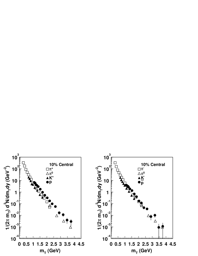
Figure 15: The transverse mass distributions of inclusive identified hadrons produced in 10% central events, including the $\pi^{0}$ as measured in the Electromagnetic Calorimeter in PHENIX and published in Adcox et al. (2002d).

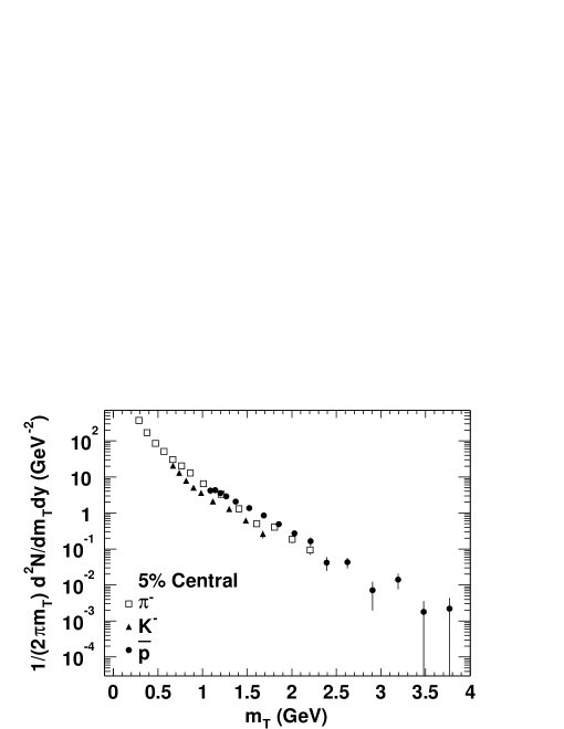
Figure 16: The transverse mass distributions of the inclusive identified hadrons produced in the 5% central events.

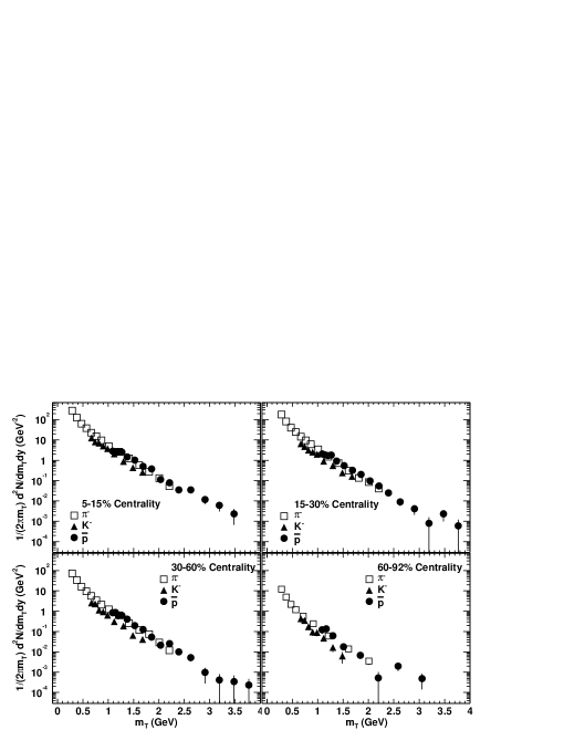
Figure 17: The transverse mass distributions of the inclusive identified hadrons produced in events with different centralities.

IV.4 SUMMED CHARGED PARTICLE MULTIPLICITY

As a consistency check we compare the measured rapidity densities as given in Section  IV.2 to previously published pseudorapidity densities of charged particles. The measured dN/dy for each hadron species is converted to dN/d$\eta$, and the total dN/d$\eta$ is calculated by summation. Figure 18 shows dN/d$\eta$ per participant nucleon pair, compared to the measurement made by PHENIX using the pad chambers alone Adcox et al. (2001b) as well as to PHOBOS and STAR yields in central collisions Back et al. (2002b); Adler et al. (2001c). We note that the lines correspond to the fit of a linear parameterization of $N_{part}$ and $N_{coll}$ to the PHENIX measurement (open circles) with $a=0.88\pm 0.28$ and $b=0.34\pm 0.12$ as described in Adcox et al. (2001c). For the 5% central collisions, we measure $598\pm 30$, and is comparable to the STAR result of $567\pm 38$ Adler et al. (2001c), the PHOBOS result of $555\pm 37$ Back et al. (2000), and the PHENIX pad chamber result of $622\pm 41$ Adcox et al. (2001b). The agreement is excellent, allowing the results of this analysis to be used to decompose the particle type dependence of the charge particle multiplicity increase with centrality.

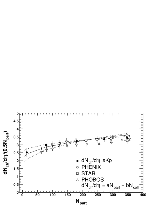
Figure 18: Both the total charged multiplicity (open) in References Adcox et al. (2001c); Adler et al. (2001c); Back et al. (2002b) and the total identified charged multiplicity (closed) scaled by the number of participant pairs are plotted together as a function of the number of participants. The lines correspond to the fit of a linear parameterization of $N_{part}$ and $N_{coll}$ to the PHENIX charged multiplicity measurement (open circles) with $a=0.88\pm 0.28$ and $b=0.34\pm 0.12$ as described in Adcox et al. (2001c).

V COMPARISON WITH MODELS

V.1 HYDRODYNAMIC-INSPIRED FIT

The charged particle pseudorapdity distributions are incompatible with a static thermal source, but the flat distribution observed in Back et al. (2000) reflects the strong longitudinal motion in the initial state. Consequently, the longitudinal momentum distribution is not an unambiguous sign of collective motion. Transverse momentum is, however, generated in the collision, so collective expansion may be more easily inferred from transverse momentum distributions.

Following the arguments of the previous section, we analyze the particle $m_{T}$ spectra. A parameterization of the $m_{T}$ distribution of particles emitted from a hydrodynamic expanding hadron source is used. In order to determine the freeze-out temperature and collective flow without confusion from hard scattering processes, a limited $p_{T}$ range is used in the fits. We include only particles with $(m_{T}-m_{0})<$ 1 GeV in the fit. Pions with $(m_{T}-m_{0})<0.38$ GeV are excluded to avoid resonance decays. All particles are assumed to decouple from the expanding hadron source Schnedermann et al. (1993) at the same freeze-out temperature, $T_{fo}$. This procedure allows us to extract $T_{fo}$ and the magnitude of the collective boost in the transverse direction.

The inverse slope includes the local temperature of a section of the hadronic matter along with its collective velocity. The simple exponential fit of Equation 10 treats each particle spectrum as a static thermal source, and a collective expansion velocity cannot be extracted reliably from a single particle spectrum. However, the relative sensitivity to the temperature and collective radial flow velocity differs for different particles. By using the information from all the particles, the expansion velocity can be inferred. We fit all particle species simultaneously with a functional form for a boosted thermal source based on relativistic hydrodynamicsSchnedermann et al. (1993).

Use of this form assumes that

• all particles decouple kinematically on a freeze-out hypersurface at the same freeze-out temperature $T_{fo}$,

• the particles collectively expand with a velocity profile increasing linearly with the radial position in the source (i.e., Hubble expansion where fluid elements do not pass through one another), and

• the particle density distribution is independent of the radial position.

Longitudinally boost invariant expansion of the particle source is also assumed.

The transverse velocity profile is parameterized as:

$$\beta_{T}(\xi)=\beta_{T}^{max}\xi^{n},$$ (13)

where $\xi=\frac{r}{R}$, and R is the maximum radius of the expanding source at freeze-out ($0<\xi<1$) Esumi et al. (1997). The maximum surface velocity is given by $\beta_{T}^{max}$, and for a linear velocity profile, n = 1. The average of the transverse velocity is equal to:

$$\langle\beta_{T}\rangle=\frac{\int{\beta_{T}^{max}\xi^{n}\xi d\xi}}{\int{\xi d\xi}}=\frac{2}{2+n}\beta_{T}^{max}.$$ (14)

Each fluid element is locally thermalized and receives a transverse boost $\rho$ that depends on the radial position as:

$$\rho=\tanh^{-1}\left(\beta_{T}\left(\xi\right)\right).$$ (15)

The $m_{T}$ dependence of the invariant yield $\frac{dN}{m_{T}dm_{T}}$ is determined by integrating over the rapidity, azimuthal angle, and radial distribution of fluid elements in the source. This procedure, discussed in Appendix  C, yields

$$\frac{d^{2}N}{m_{T}dm_{T}dy}=$$

$$A\int_{0}^{1}{m_{T}f(\xi)K_{1}\left(\frac{m_{T}\cosh(\rho)}{T_{fo}}\right)I_{0}\left(\frac{p_{T}\sinh(\rho)}{T_{fo}}\right)\xi d\xi}.$$

The parameters determined by fitting Equation 16 to the data are the freeze-out temperature $T_{fo}$, the normalization A, and the maximum surface velocity $\beta_{T}^{max}$ using a flat particle density distribution (i.e., $f(\xi)=1$).

To study the parameter correlations, we make a grid of combinations of temperature and velocity, and perform a chi-squared minimization to extract the normalization, A, for each particle type. The fit is done simultaneously for all particles in the range $(m_{T}-m_{0})<1$ GeV. In addition to this upper limit in the fit, the pion fit range includes a lower limit of $(m_{T}-m_{0})>0.38\ \rm{GeV}$ to avoid the resonance contribution to the low $p_{T}$ region (see Section  V.1.2).

The radial flow velocity and freeze-out temperature for all centralities are determined in the same way. The results are plotted together with the spectra in Figure 19. The hydrodynamic form clearly describes the spectra better than the simple exponential in Figure 14. The values for $T_{fo}$ and $\beta_{T}^{max}$ are tabulated in Table 6.

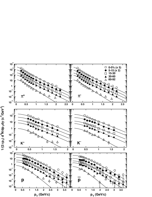
Figure 19: The parameterization and the $p_{T}$ hadron spectra for all five centrality selections.

Table 6: The minimum $\chi^{2}$ and the parameters $T_{fo}$ and $\beta_{T}^{max}$ for each of the five centrality selections. The best fit parameters are determined by averaging all parameter pairs within the 1$\sigma$ contour. The errors correspond to the standard deviation of the parameter pairs within the 1$\sigma$ $\chi^{2}$ contour. It is important to note that the fit range in Figure 19 is the same as was used to fit $m_{T}$ exponentials to the spectra in Figure 14.

Centrality (%)	$\chi^{2}$/dof	$T_{fo}$ (MeV)	$\beta_{T}^{max}$	$<\beta_{T}>$
0-5	34.0/40	$121\pm 4$	$0.70\pm 0.01$	0.47$\pm$0.01
5-15	34.7/40	$125\pm 2$	$0.69\pm 0.01$	0.46$\pm$0.01
15-30	36.2/40	$134\pm 2$	$0.65\pm 0.01$	0.43$\pm$0.01
30-60	68.9/40	$140\pm 4$	$0.58\pm 0.01$	0.39$\pm$0.01
60-92	36.3/40	$161\pm^{19}_{12}$	$0.24\pm^{0.16}_{0.2}$	0.16$\pm^{0.16}_{0.2}$

Figure 20 shows $\chi^{2}$ contours for the temperature and velocity parameters for the 5% most central collisions. The n-sigma contours are labeled up to 8$\sigma$. The $\chi^{2}$ contours indicate strong anti-correlation of the two parameters. If the freeze-out temperature decreases, the flow velocity increases. The minimum $\chi^{2}$ is $34$ and the total number of degrees of freedom (dof) is 40. The parameters that correspond to this minimum are $T_{fo}=121\pm 4$MeV and $\beta_{T}^{max}=0.70\pm 0.01$. The quoted errors are the 1$\sigma$ contour widths of $\Delta\beta_{T}^{max}$ and $\Delta T_{fo}$. Within 3$\sigma$, the $T_{fo}$ range is $106-141$ MeV and the $\beta_{T}^{max}$ range is $0.75-0.64$.

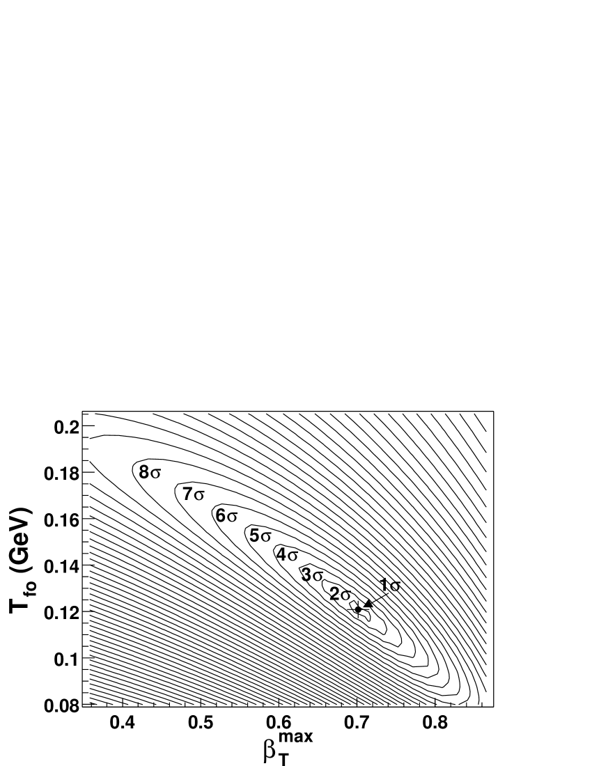
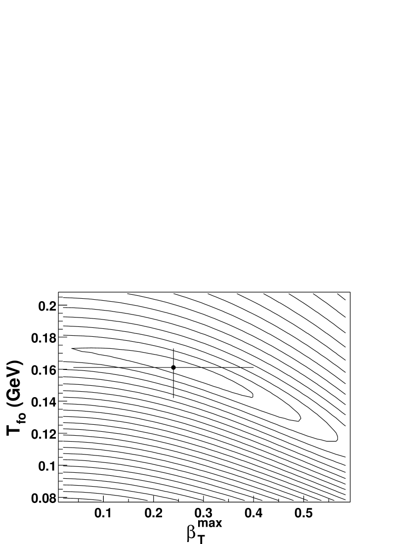
Figure 20: The $\chi^{2}$ contours in the parameter space $T_{fo}$ and $\beta_{T}^{max}$ that result after simultaneously fitting hadrons in the $0-5\%$ centrality (top) and $60-92\%$ (bottom). The n-sigma contours are labeled accordingly in the top panel. The fit results are tabulated in Table 6.

As a linear velocity profile ($n=1$ in Equation 13) is assumed, the mean flow velocity in the transverse plane is $\langle\beta_{T}\rangle=2\beta_{T}^{max}/3$. If a different particle density distribution (for instance, a Gaussian function for $f(\xi)$) were used, then the average should be determined after weighting accordingly Esumi et al. (1997).

A similar analysis for Pb+Pb collisions at 158 A GeV, was reported by the NA49 Collaboration in van Leeuwen for the NA49 Collaboration (2002). Using the same hydrodynamic parameterization, simultaneous fits of several hadron species for the highest energy results in $T_{fo}=127\pm 1$ MeV and $\beta_{T}^{max}=0.48\pm 0.01$ with $\chi^{2}/NDF=120/43$ for positive particles and $T_{fo}=114\pm 2$ MeV and $\beta_{T}^{max}=0.50\pm 0.01$ with $\chi^{2}/NDF=91/41$ for negative particles (statistical errors only). Pions and deuterons are excluded from the fits to avoid dealing with resonance contributions to the pion yield and formation of deuterons by coalescence. The $\phi$ meson is included in the fit together with the negative particles. Previously, NA49 used a different parameterization to fit the charged hadron and deuteron spectra, as well as the $m_{T}$ dependence of measured HBT source radii, resulting in overlapping $\chi^{2}$ contours with $T_{fo}=120\pm 12$ MeV and $\beta_{T}^{max}=0.55\pm 0.12$ Afanasiev et al. (1998).

V.1.1 VELOCITY AND PARTICLE DENSITY PROFILE

In order to use $\beta_{T}^{max}$ and $T_{fo}$ from the fits described above, one needs to know their sensitivity to the assumed velocity and particle density profiles in the emitting source. The choice of a linear velocity profile within the source is motivated by the profile observed in a full hydrodynamic calculation Kolb (2001a), which shows a nearly perfect linear increase of $\beta$(r) with r. Nevertheless, we also used a parabolic profile to check the sensitivity of the results to details of the velocity profile. For a parabolic velocity profile ($n=2$ in Equation 13), $\beta_{T}^{max}$ increases by $\approx$ 13% and $T_{fo}$ increases by $\approx$ 5%.

A Gaussian density profile used with a linear velocity profile increases $\beta_{T}^{max}$ by $\approx$ 2%, with a neglible difference in the temperature $T_{fo}$. As a test of the assumption that all the particles freeze out at a common temperature, the simultaneous fits were repeated without the kaons. The difference in $T_{fo}$ is within the measured uncertainties.

V.1.2 INFLUENCE OF RESONANCE PRODUCTION

The functional forms given by Equations 10 and V.1 do not include particles arising from resonance or weak decays. As resonance decays are known to result in pions at low transverse momenta Sollfrank et al. (1990); Barette et al. (1995); Boggild et al. (1996), we place a $p_{T}$ threshold of 500 MeV/c on pions included in the hydrodynamic fit. A similar approach was followed by NA44, E814, and other experiments at lower energies, which performed in-depth studies of resonance decays feeding hadron spectra. However, these were for systems with higher baryon density, so we performed a cross check on possible systematic uncertainties arising from the pion threshold used in the fits. To estimate the effect of resonance decays were they not excluded from the fit, we calculate resonance contributions following Wiedemann Wiedemann and Heinz (1997).

In order to reproduce the relative yields of different particle types, a chemical freeze-out temperature – different from the kinetic freeze-out temperature – and a baryonic chemical potential are introduced. Direct production and resonance contribution are calculated for pions and (anti)protons assuming a kinetic freeze-out temperature of 123 MeV, a transverse flow velocity of $0.612$ (equivalent to $\langle\beta_{T}\rangle=0.44$), a baryon chemical potential of 37 MeV, and a chemical freeze-out temperature (when particle production stops) of 172 MeV. These parameters are chosen as they provide a reasonable description of the (anti)proton and pion spectra and yields (10% most central) and are in good agreement with chemical freeze-out analyses Braun-Munzinger et al. (2001). Most spectra from resonance decays show a steeper fall-off than the direct production, which should lead to a smaller apparent inverse slope, depending on what fraction of the low $p_{T}$ part of the spectrum is included in the fits.

To measure the effect of resonance production on the spectral shape, the local slope is determined. For a given $m_{T}$ bin number i, the local slope is defined as

$$T_{local}\left(i\right)=-\frac{m_{T}(i+1)-m_{T}(i-1)}{\mathrm{log}[N(i+1)]-\mathrm{log}[N(i-1)]},$$ (17)

which is identical to the inverse slope independent of $m_{T}$ for an exponential.

The difference in the local slope,

$$\Delta T_{local}=T_{local}^{direct}-T_{local}^{incl},$$ (18)

is determined for direct and inclusive pions and (anti)protons. The differences are plotted as a function of $m_{T}-m_{0}$ in Figure  21. The difference in local slope for protons is below 13 MeV for the full transverse mass range; the non-monotonic behavior for protons is caused by the relatively strong transverse flow. For pions, $\Delta T_{local}$ decreases monotonically with $m_{T}$ and is below 10 MeV above $m_{T}=1\mathrm{GeV}/c$. A fit of an exponential to the pion spectra for $(m_{T}-m_{0})>0.38\ \rm{GeV}$ (which corresponds to $p_{T}>0.5$ GeV/c) yields a difference in inverse slope of 16 MeV with and without resonances.

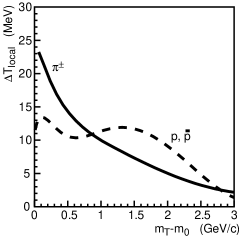
Figure 21: The difference in the local slope for direct and inclusive pions (solid) and (anti)protons (dashed).

V.2 COMPARISON WITH HYDRODYNAMIC MODELS

Hydrodynamic parameterizations as used in the previous Section rely upon many simplifying assumptions. Another approach to the study of collective flow is to compare the data to hydrodynamic models. Such models assume rapid equilibration in the collision and describe the subsequent motion of the matter using the laws of hydrodynamics. Large pressure buildup is found, and we investigate this ansatz by checking the consistency of the data with calculations using a reasonable set of initial conditions. We compare to two separate models, the hydrodynamics model of Kolb and Heinz Kolb (2001b); Kolb et al. (2000, 2001) and the “Hydro to Hadrons” (H2H) model of Teaney and Shuryak Teaney (2001); Teaney and Shuryak (2001). The H2H model consists of a hydrodynamics calculation, followed by a hadronic cascade after chemical freeze-out. The cascade step utilizes the Relativistic Quantum Molecular Dynamics (RQMD) model, developed for lower energy heavy ion collisions Sorge (1995).

In both models, initial conditions are tuned to reproduce the shape of the transverse momentum spectra measured in the most central collisions, along with the charged particle yield. Each model also includes the formation and decay of resonances.

In the Kolb and Heinz model, the initial parameters are the entropy density, baryon number density, the equilibrium time, and the freeze-out temperature which controls the duration of the expansion. The chemical freeze-out temperature is the temperature at which particle production ceases. The initial entropy or energy density and maximum temperature are fixed to match the measured multiplicity for the most central collisions using a parameterization that is tuned to produce the measured d$N_{ch}$/d$\eta$ dependence on both $N_{part}$ and $N_{coll}$. A kinetic freeze-out temperature of $T_{fo}=$ 128 MeV is used. Spectra from the Kolb-Heinz hydrodynamic model are shown in Figure 22 for pions (upper) and for protons (lower) as dotted lines. The solid lines are the results from the fits described in the previous sections. The figure thus allows two comparisons. The similarity of the dashed and solid lines shows that the hydrodynamic-inspired parameterization used to fit the data results in a $p_{T}$ distribution similar to this hydrodynamic calculation. Comparing the dashed lines to the data points shows that the hydrodynamic model agrees quite well for most of the centrality ranges. It is important to note that the model parameters are uncertain at the level of 10%, and, more importantly, the application of hydrodynamics to peripheral collisions may be less reasonable than for central collisions, as hydrodynamic calculations assume strong rescattering and a sufficiently large system size (discussed in Kolb et al. (2001)).

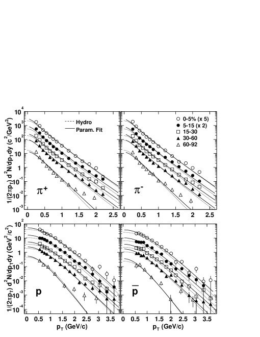
Figure 22: The hydrodynamics calculation with initial parameters tuned to match the most central spectra in the $p_{T}$ range $0.3-2.0$ GeV/c.

In reference Teaney (2001); Teaney et al. (2001), the PHENIX $\overline{p}$ spectrum shape is well described by the H2H model with the LH8 equation of state. The cascade step in the H2H model removes the requirement that all particles freeze out at a common temperature. Thus the freeze-out temperature and its profile are predicted, rather than input parameters. Furthermore, following the hadronic interactions explicitly with RQMD removes the need to rescale the particle ratios at the end of the calculation, as they are fixed by the hadronic cross sections rather than at some particular freeze-out temperature. The LH8 equation of state includes a phase transition with a latent heat of 0.8 GeV. In Teaney (2001); Teaney et al. (2001), the $\Omega$ and the $\phi$ are shown to decouple from the expanding system at $T=$ 160 MeV, and they receive a flow velocity boost of 0.45c. Pions and kaons decouple at $T=$ 135 MeV with flow velocity $=0.55$c, while protons have $T=$ 120 MeV and flow velocity $\geq$ 0.6. These temperatures and flow velocities are consistent with the values extracted from the data for the most central events. However, the average initial energy density exceeds the experimental estimate using formation time $\tau_{0}=$1 fm/c.

In Figure 23, radial flow from the fits of the previous section are shown as a function of the number of participants for $T_{fo}$ (top) and $\langle\beta_{T}\rangle$ (bottom). There is a slight decrease of $T_{fo}$, while $\langle\beta_{T}\rangle$ increases with $N_{part}$, saturating at $0.45$. The value of $\langle\beta_{T}\rangle$ from Kolb and Heinz is also shown, and agrees with the data reasonably well. In the plot of $\langle\beta_{T}\rangle$, the dashed line indicates the results of fitting the parameterization to the data while keeping $T_{fo}$ fixed at 128 MeV to agree with the value used by Kolb and Heinz. Radial flow values for central collisions remain unchanged, while those in peripheral collisions increase. Even with the extreme assumption that all collisions freeze out at the same temperature, regardless of centrality, the trend in centrality dependence of the radial flow does not change.

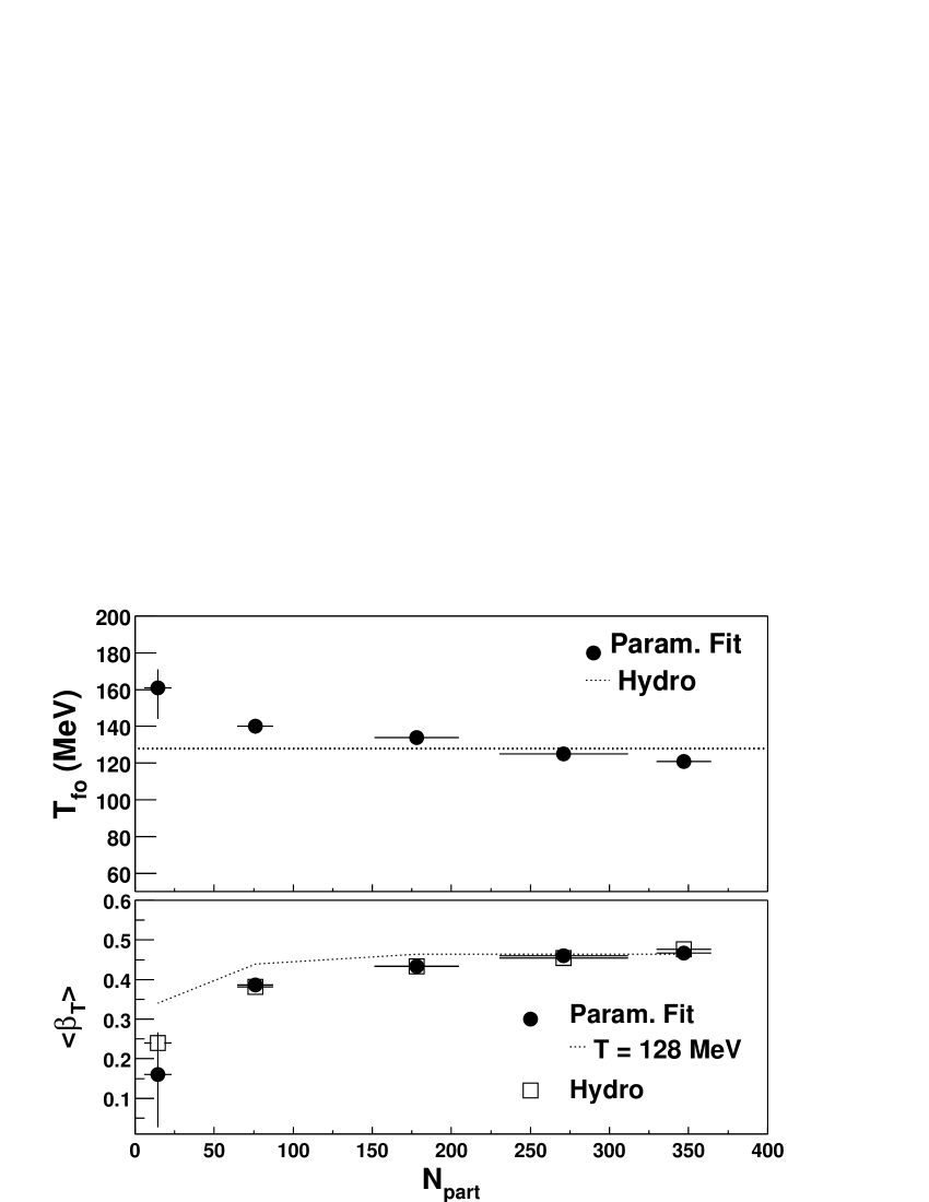
Figure 23: The expansion parameters $T_{fo}$ and $\beta_{T}^{max}$ as a function of the number of participants. As a comparison, the results from a hydrodynamic model calculation are also shown (Ref. Kolb (2001b); Kolb et al. (2000, 2001)). The dashed line corresponds to a fixed temperature of 128 MeV for all centralities in the parameterized fit to the data.

V.3 HYDRODYNAMIC CONTRIBUTIONS AT HIGHER $p_{T}$

We use the parameters extracted from the fit to the charged hadron spectra in the low $p_{T}$ region to extrapolate the effect of the soft physics to higher $p_{T}$. This yields a prediction for the spectra of hadrons should a collective expanding thermal source be the only mechanism for particle production in heavy ion collisions. Comparing this prediction to the measured spectrum of charged particles or neutral pions should indicate the $p_{T}$ range over which soft thermal processes dominate the cross section. Where the data deviate from the hydrodynamic extrapolation, other contributions, as e.g. from hard processes or non-equilibrium production become visible. The approach described here differs from hydrodynamic fits to the entire hadron spectrum, as we fix the parameters from the low $p_{T}$ region alone, where soft physics should be dominant.

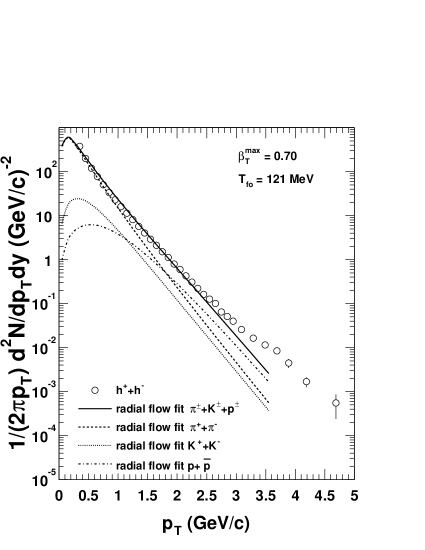
Figure 24: The high $p_{T}$ hadron spectra in Reference Adcox et al. (2002d) compared to the fit results assuming radial flow from the $\pi$Kp spectra in the 5% central events.

The hadron spectrum is calculated using the fit parameters from the low $p_{T}$ region fits shown in the preceding section, and extrapolated to higher $p_{T}$. Figure 24 shows the calculated spectrum for each particle type, and the sum of the extrapolated spectra is compared to the measured charged hadrons ($h^{+}+h^{-}$) in the 5% most central collisions. As non-identified charged hadrons are measured in $\eta$ rather than in $y$, the extrapolated spectra are converted to units of $\eta$. This conversion is most important in the low $p_{T}$ region. No additional scale factor is applied – the extrapolation and data are compared absolutely. Below $\approx$ 2.5 GeV/c $p_{T}$, the agreement is very good, while at higher $p_{T}$ the data begin to exceed the hydrodynamic extrapolation.

Other hydrodynamic calculations have been successful in describing the distributions over the full $p_{T}$ range Broniowski and Florkowski (2001) with different parameter values. There are clear indications that particle production from a hydrodynamic source, if invoked to explain the spectra at low $p_{T}$, will have a non-negligible influence even at relatively large $p_{T}$. Furthermore, the range of $p_{T}$ populated by hydrodynamically boosted hadrons is species dependent. This is clearly visible in Figure 24, which shows that the extrapolated proton spectra have a flatter $p_{T}$ distribution than the extrapolated pions and kaons. The yield of the “soft” protons reaches, and even exceeds, that of the extrapolated “soft” pions at 2 GeV/c $p_{T}$. Therefore the transition from soft to hard processes must also be species dependent, and the boost of the protons causes the region where hard processes dominate the inclusive charged particle spectrum to be at significantly higher transverse momenta in central Au+Au than in p+p collisions. Our analysis suggests this occurs not lower than $p_{T}$ = 3 GeV/c.

V.4 HADRON YIELDS AS A FUNCTION OF CENTRALITY

The previous discussion focused on the hadron spectra; now we turn to the centrality dependence of the pion, kaon, proton, and antiproton yields, which can shed further light on the importance of different mechanisms in particle production. It is instructive to see whether yields of the different hadrons scale with the number of participant nucleons, $N_{part}$, the number of binary nucleon-nucleon collisions, $N_{coll}$, or some combination of the two.

The total yields of the hadrons may be expected to be dominated by soft processes, and the wounded nucleon model of soft interactions suggests that the yields should scale as the number of participants, $N_{part}$. If each participant loses a certain fraction of its incoming energy, like e.g. in string models, where each pair of participants (or wounded nucleons) contributes a color flux tube, the total energy of the fireball formed at central rapidity would be proportional to the number of participants $N_{part}$. If, furthermore, the fireball is locally thermalized and particle production is determined at a single temperature, the multiplicity would scale with $N_{part}$. On the other hand, at very high $p_{T}$, particle production may be dominated by hard processes and scale with $N_{coll}$Kharzeev and Nardi (2001); Wang and Gyulassy (2001).

In order to investigate the existence of scaling, the multiplicities are parameterized as:

$$\frac{dN}{dy}=C\cdot(N_{part})^{\alpha_{part}}$$ (19)

and

$$\frac{dN}{dy}=C^{\prime}\cdot(N_{coll})^{\alpha_{coll}}.$$ (20)

Fit results for these parameterizations are shown in Table 7. As can be seen, the exponents $\alpha_{part}$ are $>1$ for all species, while $\alpha_{coll}$ is consistently $<1$. The production of all particles increases more strongly than with $N_{part}$, but not as strongly as with $N_{coll}$. Small differences between the different particle species are apparent: The (anti-)proton yield increases more strongly than the pion yield, and the kaon yield shows the strongest centrality dependence. Remarkably, the yield fraction scaling beyond linear with $N_{part}$ is larger for kaons, protons, and antiprotons than for pions. Perhaps it is not surprising that the yields do not scale simply with $N_{part}$; the collective flow seen in the $p_{T}$ spectra already shows that the nucleon-nucleon collisions cannot be independent.

Table 7: Fit parameters for each particle species using equations 19 and 20.

particle	$\alpha_{part}$	$\alpha_{coll}$
$\pi^{+}$	$1.06\pm 0.01$	$0.79\pm 0.01$
$\pi^{-}$	$1.08\pm 0.01$	$0.80\pm 0.01$
$K^{+}$	$1.18\pm 0.02$	$0.88\pm 0.02$
$K^{-}$	$1.20\pm 0.03$	$0.89\pm 0.02$
$p^{+}$	$1.16\pm 0.02$	$0.86\pm 0.02$
$p^{-}$	$1.14\pm 0.03$	$0.84\pm 0.02$

We next check whether the simple model of hadron yields can be brought into agreement with the data by adding a component of the yields scaling as the number of binary collisions, $N_{coll}$. Such an admixture inspires simple two-component models Kharzeev and Nardi (2001); Wang and Gyulassy (2001). The nonlinearity of dN/dy on the number of participants is illustrated by the ratio (dN/dy)/$N_{part}$, shown in Figure 25 as a function of centrality. The yields are seen to depend linearly on $N_{coll}/N_{part}$. As seen already from the exponents in Table 7, the increase with centrality is strongest for kaons, intermediate for (anti-)protons, and weakest for pions. This indicates that protons and antiprotons have a larger component scaling with $N_{coll}$ than pions.

We fit the yields per participant with Equation  21. As in Kharzeev and Nardi (2001); Wang and Gyulassy (2001) we parameterize the multiplicity using two free parameters: $n_{pp}$, the multiplicity in p+p collisions, and $x$, the relative strength of the component scaling with $N_{coll}$.

$$R\equiv{dN/dy\over N_{part}} = (1-x)\cdot n_{pp}\frac{1}{2}+x\cdot n_{pp}\frac{N_{coll}}{N_{part}}$$ (21)

$$= n_{pp}\left[\frac{1}{2}+x\left(\frac{N_{coll}}{N_{part}}-\frac{1}{2}\right)\right].$$

The results of the fit are shown as solid lines in Figure 25. The fit parameter values are given in Table 8. All hadron species are well fit. The importance of the component scaling as $N_{coll}$ is largest for kaons and smallest for pions.

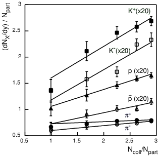
Figure 25: $dN/dy$ per participant of different particle species as a function of the number of collisions per participant. Kaon and (anti-)proton multiplicities are scaled by a factor of 20.

Table 8: Values of the parameters $n_{pp}$ and $x$ from fitting Equation 21 to the observed dN/dy per $N_{part}$.

	$n_{pp}$	$x$
$\pi^{+}$	$1.41\pm 0.11$	$0.028\pm 0.020$
$\pi^{-}$	$1.10\pm 0.11$	$0.085\pm 0.030$
$K^{+}$	$0.130\pm 0.021$	$0.232\pm 0.076$
$K^{-}$	$0.089\pm 0.020$	$0.326\pm 0.132$
$p$	$0.089\pm 0.013$	$0.181\pm 0.062$
$\overline{p}$	$0.062\pm 0.010$	$0.172\pm 0.068$

We check the consistency of the fits in Figure 25 with known hadron yields in p+p collisions by extrapolating the fits down to two participants (and one binary nucleon-nucleon collision). Isospin differences between p+p and Au+Au are ignored. The check is done by separately extrapolating the fitted fraction of yield which scales with $N_{coll}$ and the fraction scaling with $N_{part}$ down to one nucleon-nucleon collision and two participant nucleons, and summing the result. One obtains particle ratios of $K/\pi=(8.7\pm 2.6)\%$ and $\bar{p}/\pi=(4.9\pm 0.8)\%$. These values fall between those measured at lower $\sqrt{s}$ at the ISR Alper et al. (1975c) and those at higher $\sqrt{s}$ at the Tevatron Alexopoulos et al. (1993), as expected since the RHIC energy lies in between. Thus the Au+Au data are shown to scale down to p+p reasonably.

One may expect that the particle ratios at very high $p_{T}$ should be dominated by hard scattering, and therefore scale with the number of binary collisions. Consequently, we look at ratios of the $N_{coll}$ scaling components alone, extrapolated down to one binary collision. The values are compared to measurements of hadron ratios at the ISR Alper et al. (1975d) in Figures 26 and 27. The ratio of the extrapolated Au+Au yield fractions scaling as $N_{coll}$ are shown as solid lines for $p_{T}\geq 2\,\mathrm{GeV}/c$. The agreement with the p+p data at high $p_{T}$ is quite good.

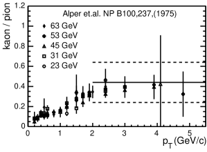
Figure 26: Kaon to pion ratio as a function of $p_{T}$. The different points are measured in $p+p$ collisions (data from ref. Alper et al. (1975d)). The solid line is the asymptotic value for high $p_{T}$ in p+p derived from the hard scattering component of the fits using Equation  21 to the measured centrality dependence of dN/dy in Au-Au collisions at $\sqrt{s_{NN}}=130$ GeV. The dashed lines indicate the corresponding uncertainty.

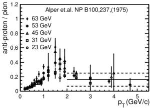
Figure 27: Antiproton to $\pi^{-}$ ratio as a function of $p_{T}$. The different points are measured in $p+p$ collisions (data from ref. Alper et al. (1975d)). The solid line is the asymptotic value for high $p_{T}$ in p+p derived from the hard scattering component of the fits using Equation  21 to the measured centrality dependence of dN/dy in Au-Au collisions at $\sqrt{s_{NN}}=130$ GeV. The dashed lines indicate the corresponding uncertainty.

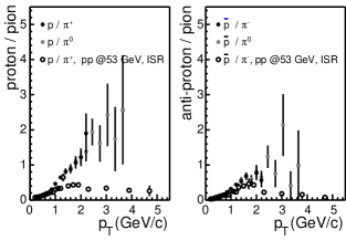
Figure 28: a) Proton to pion ratio as a function of $p_{T}$. b) Antiproton to pion ratio as a function of $p_{T}$. The open circles represent measurements in $p+p$ collisions (data from ref. Alper et al. (1975d)). The filled circles show the 10 $\%$ most central Au+Au collisions. The neutral pion spectra are from the data published in Adcox et al. (2002d).

Finally, we directly compare p/$\pi$ and $\overline{p}/\pi$ ratios in central Au+Au collisions with p+p, as a function of $p_{T}$. These ratios from the $10\%$ most central data, using the charged particle measurement from this paper and neutral pions from Adcox et al. (2002d), are shown in Figure 28. The ratios show a steady increase up to 2.5 GeV/c in $p_{T}$. Even though the simple extrapolation of the $N_{coll}$ scaling yield fraction agreed with p+p, the ratios of the full yield significantly exceed those in the ISR measurements Alper et al. (1975d). According to Gyulassy and collaborators, Vitev and Gyulassy (2002), this result may give insight into baryon number transport and the interplay between soft and hard processes.

Of course, splitting the observed yields into portions which scale with $N_{part}$ and $N_{coll}$ is by no means a unique explanation of the data. The spectra and yields can also be well reproduced by thermal models, which break such simple scalings due to the multiple interactions suffered by the constituents.

Simple thermal models that ignore transverse and longitudinal flow Kampfer et al. (2002) are able to describe the centrality dependence of the mid-rapidity $\pi^{\pm}$, $K^{\pm}$, $p$, and $\overline{p}$ yields by tuning the chemical freeze-out temperature $T_{ch}$, the baryon chemical potential $\mu_{B}$ and by introducing a strangeness saturation factor $\gamma_{s}$. It was found that $\mu_{B}$ is independent of centrality, while both $\gamma_{s}$ and $T_{ch}$ increase from peripheral to central collisions. Within the same model, the centrality dependence of the particle yields at lower energy ($\sqrt{s_{NN}}=17$ GeV  Sikler (1999); Freise (2002)) are described by constant $T_{ch}$ and $\mu_{B}$. The strong centrality dependence in kaon production at both energies is accounted for by the increase in the strangeness saturation factor $\gamma_{s}$. Although the integrated particle yields are very well described, such simple thermal models do not attempt a comparison to the single particle spectra, which clearly indicate centrality dependent flow effects not included in the model.

Thermal models which include hydrodynamical parameters on a freeze-out hypersurface to account for longitudinal and transverse flow can reproduce the absolutely normalized particle spectra by introducing only two thermal parameters $T_{ch}$ and $\mu_{B}$  Broniowski et al. (2002); Broniowski and Florkowski (2002). In this approach, the thermal parameters are independent of centrality, while the geometric parameters are adjusted to reproduce the spectra. Good agreement with the data is obtained up to $p_{T}\approx 2-3$ GeV/c, however an explicit comparison with the centrality dependence of the integrated mid-rapidity yields has not yet been made.

This section shows that the yields of all hadrons increase more rapidly than linearly with the number of participants, but the increase is weaker than scaling with the number of binary collisions. The excess beyond linear scaling with $N_{part}$ is strongest for kaons, intermediate for (anti-)protons, and weakest for pions. The centrality dependence of the total yields can be well fit with a sum of these two kinds of scaling. At high $p_{T}$, the baryon and anti-baryon yields greatly exceed expectations from p+p collisions. Thermal models, which do not invoke strict scaling rules, can successfully reproduce the data as well, providing that they include the radial flow required by the $p_{T}$ spectra.

VI SUMMARY AND CONCLUSION

We have presented the spectra and yields of identified hadrons produced in $\sqrt{s_{NN}}=$ 130 GeV Au + Au collisions. The yields of pions increase approximately linearly with the number of participant nucleons, while the yield increase is faster than linear for kaons, protons, and antiprotons.

Hydrodynamic analyses of the particle spectra are performed: the spectra are fit with a hydrodynamic-inspired parameterization to extract freeze-out temperature and radial flow velocity of the particle source. The data are also compared to two full hydrodynamics calculations. The simultaneous fits of pion, kaon, proton, and antiproton spectra show that radial flow in central collisions at RHIC exceeds that at lower energies and increases with centrality of the collision. The hydrodynamic models are consistent with the measured spectral shapes, extracted freeze-out temperature $T_{fo}$, and the flow velocity $\beta_{T}$ in central collisions.

Extrapolating the fits to estimate thermal particle production at higher $p_{T}$ allows us to study the soft-hard physics boundary by comparing to measured spectra at high $p_{T}$. The yield of the “soft” protons reaches, and even exceeds, that of the extrapolated “soft” pions at 2 GeV/c $p_{T}$. The sum of the extrapolated “soft” spectra agree with the measured inclusive data to $p_{T}$ $\approx 2.5-3$ GeV/c. The transition from soft to hard processes must be species dependent, and the admixture of boosted nucleons implies that hard processes do not dominate the inclusive charged particle spectra until approximately 3 GeV/c.

Appendix A Determining $N_{part}$ and $N_{coll}$

As only the fraction of the total cross section is measured in both the ZDC and BBC detectors, a model-dependent calculation is used to map collision centrality to the number of participant nucleons, $N_{part}$, and the number of nucleons undergoing binary collisions, $N_{coll}$. A discussion of this calculation at RHIC can be found elsewhere Kharzeev and Nardi (2001).

Table 9: Invariant yields for $\pi^{\pm}$, $K^{\pm}$, and (anti)p measured in minimum bias events at midrapidity and normalized to one rapidity unit. The errors are statistical only.

$p_{T}$ (GeV/c)	$\pi^{\pm}$	$K^{\pm}$	p($\overline{p}$)
0.25	112$\pm$2
	109$\pm$2
0.35	56 $\pm$1
	49.9 $\pm$0.9
0.45	28.0 $\pm$0.5	6.1$\pm$0.4
	24.1 $\pm$0.5	4.6$\pm$0.4
0.55	15.7 $\pm$0.3	4.0$\pm$0.3	2.3$\pm$ 0.1
	14.6 $\pm$0.3	3.2$\pm$0.2	1.2$\pm$0.1
0.65	9.1 $\pm$0.2	2.8$\pm$0.2	1.8$\pm$ 0.1
	8.7 $\pm$0.2	2.1 $\pm$0.2	1.17$\pm$ 0.09
0.75	5.8 $\pm$0.1	1.7$\pm$0.1	1.38$\pm$ 0.08
	5.6 $\pm$0.2	1.6$\pm$0.1	0.98$\pm$0.07
0.85	3.8 $\pm$0.1	1.30$\pm$0.08	1.18$\pm$0.07
	3.6$\pm$0.1	1.17$\pm$0.09	0.95$\pm$0.07
0.95	2.40 $\pm$0.08	0.87$\pm$0.06	0.98$\pm$ 0.06
	2.28 $\pm$0.08	0.69$\pm$0.06	0.65$\pm$ 0.05
1.05	1.61 $\pm$0.06	0.62$\pm$0.04	0.70$\pm$ 0.04
	1.61 $\pm$0.06	0.53$\pm$0.05	0.50$\pm$ 0.04
1.15	1.03 $\pm$0.04	0.43$\pm$0.03	0.60$\pm$ 0.04
	1.17 $\pm$0.05	0.38$\pm$0.04	0.35$\pm$ 0.03
1.25	0.71$\pm$0.03	0.33$\pm$0.03	0.41$\pm$ 0.03
	0.76 $\pm$0.04	0.27$\pm$0.03	0.34$\pm$0.03
1.35	0.46 $\pm$0.02	0.20$\pm$0.02	0.32$\pm$0.02
	0.54$\pm$0.03	0.16$\pm$0.02	0.22$\pm$0.02
1.45	0.35$\pm$0.02	0.17$\pm$0.02	0.23$\pm$ 0.02
	0.31 $\pm$0.02	0.13$\pm$0.02	0.18$\pm$ 0.02
1.55	0.24 $\pm$0.02	0.10$\pm$0.01	0.17$\pm$ 0.02
	0.22 $\pm$0.02	0.10$\pm$0.01	0.15$\pm$ 0.02
1.65	0.16 $\pm$0.01	0.08$\pm$0.01
	0.15 $\pm$0.01	0.07$\pm$0.01
1.70			0.119$\pm$ 0.008
			0.080$\pm$ 0.007
1.75	0.11 $\pm$0.01
	0.11 $\pm$0.01
1.85	0.079 $\pm$0.008
	0.092 $\pm$0.009
1.90			0.068$\pm$ 0.006
			0.041$\pm$ 0.005
1.95	0.063 $\pm$0.007
	0.066 $\pm$0.008
2.05	0.036 $\pm$0.005
	0.034 $\pm$0.005
2.10			0.036$\pm$ 0.004
			0.022$\pm$ 0.003
2.15	0.026 $\pm$0.004
	0.025 $\pm$0.004
2.25	0.015 $\pm$0.003
	0.020 $\pm$0.004
2.30			0.020$\pm$ 0.003
			0.012$\pm$ 0.002
2.50			0.010$\pm$ 0.002
			0.011$\pm$ 0.002
2.70			0.006$\pm$ 0.001
			0.0026$\pm$ 0.0009
2.90			0.0035$\pm$ 0.0008
			0.003$\pm$ 0.001
3.10			0.0028$\pm$ 0.0007
			0.0011$\pm$ 0.0005
3.30			0.0014$\pm$ 0.0005
			0.0010$\pm$ 0.0004

Using a Glauber model combined with a simulation of the BBC and ZDC responses, $N_{part}$ and $N_{coll}$ are determined in each centrality. The model provides the thickness of nuclear matter in the direct path of each oncoming nucleon, and uses the inelastic nucleon-nucleon cross section $\sigma^{inel}_{N+N}$ to determine whether or not a nucleon-nucleon collision occurs. We assume the following:

• The nucleons travel in straight-line paths, parallel to the velocity of its respective nucleus.

• An inelastic collision occurs if the relative distance between two nucleons is less than $\sqrt{\sigma^{inel}_{N+N}/\pi}$.

• Fluctuations are introduced by using the simulated detector response for both the ZDC and BBC.

In this calculation, the Woods-Saxon nuclear density distribution ($\rho(r)$) is used for each nucleus with three parameters, the nuclear radius R $=6.38^{+0.27}_{-0.13}$ fm, diffusivity d $=0.53\pm 0.01$ fm Glauber and Natthiae (1970), and the inelastic nucleon-nucleon cross section $\sigma^{inel}_{N+N}$ $=$ 40 $\pm$ 3 mb,

$$\rho(r)=\frac{\rho_{0}}{1+e^{\frac{r-r_{n}}{d}}}.$$ (22)

Appendix B Invariant Cross Sections

Tabulated here are the measured invariant yields of pions, kaons, and (anti)protons produced in Au+Au collisions at 130 GeV. The first set of tables (Tables  9- 12) are the invariant cross sections plotted in Figures 9 and 10. The second set of tables (Tables  13- 16) are the invariant cross sections in equal $p_{T}$ bins as used in Figure 11.

Table 10: Pion invariant yields in each event centrality and $p_{T}$ bin measured at midrapidity, normalized to one rapidity unit. For each measured $p_{T}$ bin, the positive pion cross section is the top row and the negative pion cross section is the bottom row. Errors are statistical only.

$p_{T}$ (GeV/c)	0-5%	5-15%	15-30%	30-60%	60-92%
0.25	355 $\pm$ 9	282 $\pm$ 6	186 $\pm$ 4	81 $\pm$ 2	13.2 $\pm$ 0.5
	371 $\pm$ 10	275 $\pm$ 7	180 $\pm$ 4	74 $\pm$ 2	12.1 $\pm$ 0.5
0.35	188 $\pm$ 5	146 $\pm$ 3	93 $\pm$ 2	36.6 $\pm$ 0.8	5.3 $\pm$ 0.2
	169 $\pm$ 5	128 $\pm$ 3	82 $\pm$ 2	34.3 $\pm$ 0.9	5.0 $\pm$ 0.2
0.45	95 $\pm$ 3	74 $\pm$ 2	48 $\pm$ 1	17.5 $\pm$ 0.5	2.7 $\pm$ 0.1
	86 $\pm$ 3	63 $\pm$ 2	40 $\pm$ 1	15.7 $\pm$ 0.5	2.1 $\pm$ 0.1
0.55	56 $\pm$ 2	41 $\pm$ 1	26.0 $\pm$ 0.7	10.1 $\pm$ 0.3	1.32 $\pm$ 0.09
	51 $\pm$ 2	38 $\pm$ 1	24.5 $\pm$ 0.8	9.6 $\pm$ 0.3	1.18 $\pm$ 0.09
0.65	32$\pm$ 1	25.6 $\pm$ 0.8	15.0 $\pm$ 0.5	5.3 $\pm$ 0.2
	30 $\pm$ 1	22.6 $\pm$ 0.8	14.5 $\pm$ 0.5	5.7 $\pm$ 0.2
0.70					0.62$\pm$ 0.04
					0.57$\pm$ 0.04
0.75	21.1 $\pm$ 0.9	15.4 $\pm$ 0.6	9.9 $\pm$ 0.4	3.6 $\pm$ 0.1
	20 $\pm$ 1	15.3 $\pm$ 0.6	9.5 $\pm$ 0.4	3.5 $\pm$ 0.2
0.85	14.0 $\pm$ 0.7	10.3 $\pm$ 0.4	6.4 $\pm$ 0.3	2.3 $\pm$ 0.1
	12.8 $\pm$ 0.8	9.6 $\pm$ 0.5	6.1 $\pm$ 0.3	2.1 $\pm$ 0.1
0.90					0.19 $\pm$ 0.02
					0.24 $\pm$ 0.02
1.00	7.1 $\pm$ 0.3	5.3$\pm$ 0.2	3.4 $\pm$ 0.1	1.25 $\pm$ 0.05
	6.5 $\pm$ 0.3	5.0 $\pm$ 0.2	3.4 $\pm$ 0.1	1.25 $\pm$ 0.05
1.20	3.2 $\pm$ 0.2	2.2 $\pm$ 0.1	1.47 $\pm$ 0.07	0.55 $\pm$ 0.03	0.064 $\pm$ 0.006
	3.3 $\pm$ 0.2	2.6 $\pm$ 0.1	1.51 $\pm$ 0.08	0.63 $\pm$ 0.04	0.061 $\pm$ 0.007
1.40	1.3 $\pm$ 0.1	1.01 $\pm$ 0.07	0.72 $\pm$ 0.04	0.27 $\pm$ 0.02
	1.3 $\pm$ 0.1	1.25 $\pm$ 0.09	0.72 $\pm$ 0.05	0.26 $\pm$ 0.02
1.60	0.55 $\pm$ 0.07	0.57 $\pm$ 0.05	0.33 $\pm$ 0.03	0.14 $\pm$ 0.01	0.015 $\pm$ 0.003
	0.51 $\pm$ 0.07	0.57 $\pm$ 0.05	0.30 $\pm$ 0.03	0.12 $\pm$ 0.01	0.014 $\pm$ 0.003
1.80	0.35 $\pm$ 0.05	0.25 $\pm$ 0.03	0.15 $\pm$ 0.02	0.060 $\pm$ 0.008
	0.40 $\pm$ 0.06	0.27 $\pm$ 0.03	0.14 $\pm$ 0.02	0.075 $\pm$ 0.009
2.00	0.18 $\pm$ 0.03	0.13 $\pm$ 0.02	0.10 $\pm$ 0.01	0.023 $\pm$ 0.004	0.005 $\pm$ 0.001
	0.18 $\pm$ 0.04	0.13 $\pm$ 0.02	0.09 $\pm$ 0.01	0.029 $\pm$ 0.005	0.004$\pm$ 0.001
2.20	0.043 $\pm$ 0.02	0.07 $\pm$ 0.01	0.034 $\pm$ 0.007	0.012 $\pm$ 0.003
	0.09 $\pm$ 0.03	0.05 $\pm$ 0.01	0.042 $\pm$ 0.009	0.012 $\pm$ 0.003

Table 11: Kaon invariant yields in each event centrality and $p_{T}$ bin, measured at midrapidity and normalized to one rapidity unit. The top row in each $p_{T}$ bin is $K^{+}$, and the bottom row is $K^{-}$. Errors are statistical only.

$p_{T}$ (GeV/c)	0-5%	5-15%	15-30%	30-60%	60-92%
0.44					0.5 $\pm$ 0.1
					0.4 $\pm$ 0.1
0.45	21$\pm$ 3	16 $\pm$ 2	10 $\pm$ 1	4.3 $\pm$ 0.5
	21$\pm$ 3	13 $\pm$ 2	7 $\pm$ 1	2.5 $\pm$ 0.4
0.54					0.20 $\pm$ 0.07
					0.3 $\pm$ 0.1
0.55	15$\pm$ 2	11 $\pm$ 1	6.6 $\pm$ 0.7	2.4 $\pm$ 0.3
	13$\pm$ 2	8 $\pm$ 1	4.8 $\pm$ 0.6	2.3 $\pm$ 0.3
0.65	9 $\pm$ 1	7.5 $\pm$ 0.7	4.7 $\pm$ 0.4	1.9 $\pm$ 0.2
	8 $\pm$ 1	7.0 $\pm$ 0.8	3.1 $\pm$ 0.4	1.1 $\pm$ 0.2
0.69					0.18 $\pm$ 0.03
					0.14 $\pm$ 0.03
0.75	5.3 $\pm$ 0.7	4.6 $\pm$ 0.5	3.1 $\pm$ 0.3	0.9 $\pm$ 0.1
	5.1 $\pm$ 0.8	5.0 $\pm$ 0.6	2.5 $\pm$ 0.3	0.9 $\pm$ 0.1
0.85	5.7 $\pm$ 0.7	3.6 $\pm$ 0.4	2.1 $\pm$ 0.2	0.67 $\pm$ 0.08
	3.6 $\pm$ 0.6	3.7 $\pm$ 0.4	2.0 $\pm$ 0.2	0.64 $\pm$ 0.09
0.89					0.07 $\pm$ 0.02
					0.09 $\pm$ 0.02
0.95	3.0 $\pm$ 0.4	2.3 $\pm$ 0.2	1.5 $\pm$ 0.2	0.51 $\pm$ 0.07
	2.4 $\pm$ 0.4	2.3 $\pm$ 0.3	1.0 $\pm$ 0.2	0.35 $\pm$ 0.06
1.05	2.3 $\pm$ 0.3	1.5 $\pm$ 0.2	1.2 $\pm$ 0.1	0.37 $\pm$ 0.05
	1.8 $\pm$ 0.3	1.8 $\pm$ 0.2	0.8 $\pm$ 0.1	0.27 $\pm$ 0.05
1.15	1.6 $\pm$ 0.3	1.3 $\pm$ 0.2	0.62 $\pm$ 0.09	0.29 $\pm$ 0.04
	1.4 $\pm$ 0.3	0.9 $\pm$ 0.2	0.7 $\pm$ 0.1	0.23 $\pm$ 0.04
1.17					0.012$\pm$ 0.004
					0.015$\pm$ 0.005
1.25	1.1 $\pm$ 0.2	1.0 $\pm$ 0.1	0.66 $\pm$ 0.09	0.15 $\pm$ 0.03
	1.2 $\pm$ 0.2	0.8 $\pm$ 0.1	0.41 $\pm$ 0.08	0.15 $\pm$ 0.03
1.35	0.6 $\pm$ 0.1	0.6 $\pm$ 0.1	0.35 $\pm$ 0.05	0.12 $\pm$ 0.02
	0.9 $\pm$ 0.2	0.5 $\pm$ 0.1	0.22 $\pm$ 0.05	0.05 $\pm$ 0.02
1.45	0.5 $\pm$ 0.1	0.45 $\pm$ 0.08	0.32 $\pm$ 0.05	0.10 $\pm$ 0.02
	0.4 $\pm$ 0.1	0.36 $\pm$ 0.08	0.26 $\pm$ 0.05	0.07 $\pm$ 0.02
1.55	0.4 $\pm$ 0.1	0.26 $\pm$ 0.06	0.14 $\pm$ 0.03	0.07 $\pm$ 0.02
	0.4 $\pm$ 0.1	0.28 $\pm$ 0.07	0.21 $\pm$ 0.04	0.04 $\pm$ 0.01
1.57					0.008$\pm$ 0.002
					0.004$\pm$ 0.002
1.65	0.4 $\pm$ 0.1	0.24 $\pm$ 0.05	0.10 $\pm$ 0.03	0.05 $\pm$ 0.01
	0.12 $\pm$ 0.06	0.23 $\pm$ 0.06	0.12 $\pm$ 0.03	0.04 $\pm$ 0.01

Table 12: (Anti)proton invariant yields in each event centrality and $p_{T}$ bin, measured at midrapidity and normalized to one rapidity unit. The top row in each $p_{T}$ is the proton cross section, and the bottom row the antiproton. The errors are statistical only.

$p_{T}$ (GeV/c)	0-5%	5-15%	15-30%	30-60%	60-92%
0.545					0.26 $\pm$ 0.06
					0.12 $\pm$ 0.05
0.55	8 $\pm$ 1	4.9 $\pm$ 0.5	4.0 $\pm$ 0.4	1.6 $\pm$ 0.2
	4.2 $\pm$ 0.8	2.8 $\pm$ 0.5	2.0 $\pm$ 0.3	0.8 $\pm$ 0.1
0.65	6.3 $\pm$ 0.7	4.7 $\pm$ 0.4	2.7 $\pm$ 0.2	1.2 $\pm$ 0.1
	4.3 $\pm$ 0.7	2.6 $\pm$ 0.4	1.9 $\pm$ 0.3	0.9 $\pm$ 0.1
0.695					0.14 $\pm$ 0.02
					0.14 $\pm$ 0.03
0.75	4.4 $\pm$ 0.5	4.0 $\pm$ 0.4	2.2 $\pm$ 0.2	0.90 $\pm$ 0.08
	3.6 $\pm$ 0.5	2.5 $\pm$ 0.3	1.7 $\pm$ 0.2	0.60 $\pm$ 0.08
0.85	3.9 $\pm$ 0.4	3.3 $\pm$ 0.3	1.9 $\pm$ 0.2	0.75 $\pm$ 0.07
	2.9 $\pm$ 0.5	2.5 $\pm$ 0.3	1.8 $\pm$ 0.2	0.62$\pm$ 0.08
0.895					0.10$\pm$ 0.02
					0.06$\pm$ 0.01
1.00	3.1 $\pm$ 0.2	2.4 $\pm$ 0.2	1.37 $\pm$ 0.09	0.46 $\pm$ 0.03
	2.1 $\pm$ 0.2	1.5 $\pm$ 0.1	0.91 $\pm$ 0.08	0.41 $\pm$ 0.04
1.18					0.031$\pm$ 0.005
					0.018$\pm$ 0.004
1.20	2.0 $\pm$ 0.2	1.4 $\pm$ 0.1	0.82 $\pm$ 0.06	0.28 $\pm$ 0.02
	1.4$\pm$ 0.2	1.0 $\pm$ 0.1	0.54 $\pm$ 0.05	0.19 $\pm$ 0.02
1.40	1.1 $\pm$ 0.1	0.74 $\pm$ 0.07	0.46 $\pm$ 0.04	0.14 $\pm$ 0.01
	0.9 $\pm$ 0.1	0.50 $\pm$ 0.06	0.32 $\pm$ 0.04	0.13 $\pm$ 0.02
1.58					0.005$\pm$ 0.002
					0.007$\pm$ 0.002
1.60	0.54 $\pm$ 0.07	0.49 $\pm$ 0.05	0.25 $\pm$ 0.03	0.09 $\pm$ 0.01
	0.49 $\pm$ 0.08	0.37 $\pm$ 0.05	0.20 $\pm$ 0.03	0.053 $\pm$ 0.009
1.80	0.34 $\pm$ 0.05	0.25 $\pm$ 0.03	0.16 $\pm$ 0.02	0.047 $\pm$ 0.007
	0.27 $\pm$ 0.06	0.11 $\pm$ 0.02	0.10 $\pm$ 0.02	0.021 $\pm$ 0.005
1.98					0.003 $\pm$ 0.001
					0.0005 $\pm$ 0.0005
2.00	0.20 $\pm$ 0.04	0.12 $\pm$ 0.02	0.10 $\pm$ 0.01	0.029 $\pm$ 0.005
	0.16 $\pm$ 0.04	0.08 $\pm$ 0.02	0.05 $\pm$ 0.01	0.026 $\pm$ 0.006
2.20	0.13 $\pm$ 0.03	0.08 $\pm$ 0.02	0.05 $\pm$ 0.01	0.008 $\pm$ 0.002
	0.04 $\pm$ 0.02	0.03 $\pm$ 0.01	0.025 $\pm$ 0.007	0.010 $\pm$ 0.003
2.41					0.0010 $\pm$ 0.0006
					0.0020 $\pm$ 0.0008
2.425	0.06 $\pm$ 0.02	0.05 $\pm$ 0.01	0.017 $\pm$ 0.005	0.007 $\pm$ 0.002
	0.05 $\pm$ 0.02	0.04 $\pm$ 0.01	0.011 $\pm$ 0.004	0.006$\pm$ 0.002
2.675	0.014 $\pm$ 0.008	0.019 $\pm$ 0.006	0.010 $\pm$ 0.003	0.004 $\pm$ 0.001
	0.005 $\pm$ 0.005	0.018 0.007	0.002 0.002	0.0012 $\pm$ 0.0008
2.908					0.0006 $\pm$ 0.0004
					0.0005 $\pm$ 0.0003
2.925	0.017 $\pm$ 0.007	0.006 $\pm$ 0.003	0.006 $\pm$ 0.002	0.003 $\pm$ 0.001
	0.020 $\pm$ 0.009	0.009 $\pm$ 0.004	0.003 $\pm$ 0.002	0.0009 $\pm$ 0.0006
3.175	0.013 $\pm$ 0.006	0.002 $\pm$ 0.002	0.003 $\pm$ 0.002	0.0012 $\pm$ 0.0007
	0.006 $\pm$ 0.004	0.003 $\pm$ 0.002	0.0010 $\pm$ 0.001
3.425	0.004 $\pm$ 0.003	0.003 $\pm$ 0.002	0.002 $\pm$ 0.001	0.0007 $\pm$ 0.0005
	0.002 $\pm$ 0.002	0.001 $\pm$ 0.001	0.002 $\pm$ 0.001	0.0003 $\pm$ 0.0003
3.675	0.003 $\pm$ 0.003			0.0003 $\pm$ 0.0003
	0.003 $\pm$ 0.003		0.0008 $\pm$ 0.0008

Table 13: Minimum bias invariant yields for all particles in equal $p_{T}$ bins. For each $p_{T}$, the first line are the positive particle yields, and the second are the negative particle yields. The units are $c^{2}/GeV^{2}$.

$p_{T}(GeV/c)$	$\pi^{\pm}$	$K^{\pm}$	(anti)p
0.25	112$\pm$2
	109$\pm$2
0.35	56 $\pm$1
	49.9 $\pm$0.9
0.45	28.0 $\pm$0.5	6.1$\pm$0.4
	24.1 $\pm$0.5	4.6$\pm$0.4
0.55	15.7 $\pm$0.3	4.0$\pm$0.3	2.3$\pm$0.1
	14.6 $\pm$0.3	3.2$\pm$0.2	0.38$\pm$0.02
0.70	7.3 $\pm$0.1	2.18$\pm$0.09	1.55$\pm$0.06
	7.0 $\pm$0.1	1.9$\pm$0.1	1.07$\pm$0.06
0.90	3.06 $\pm$0.06	1.07$\pm$0.05	1.08$\pm$0.04
	2.89 $\pm$0.07	0.91$\pm$0.05	0.79$\pm$0.04
1.20	0.91 $\pm$0.02	0.38$\pm$0.02	0.49$\pm$0.02
	0.98 $\pm$0.02	0.32$\pm$0.02	0.35$\pm$0.01
1.60	0.208 $\pm$0.007	0.104$\pm$0.006	0.157$\pm$0.007
	0.193 $\pm$0.007	0.093$\pm$0.006	0.119$\pm$0.007
2.00	0.050 $\pm$0.003		0.051$\pm$0.003
	0.053 $\pm$0.003		0.031$\pm$0.003
2.45	0.0028 $\pm$0.0005		0.013$\pm$0.001
	0.0034 $\pm$0.0006		0.009$\pm$0.001
2.95			0.0036$\pm$0.0006
			0.0022$\pm$0.0005
3.55			0.0007$\pm$0.0002
			0.0006$\pm$0.0002

Table 14: Pion invariant yields in each event centrality normalized to one rapidity unit at midrapidity. The first line corresponds to positive pions, and the second to negative pions.

$p_{T}$ (GeV/c)	0-5%	5-15%	15-30%	30-60%	60-92%
0.25	355$\pm$9	282$\pm$6	186$\pm$4	81$\pm$2	13.2$\pm$0.5
	371$\pm$10	275$\pm$7	180$\pm$ 4	74 $\pm$ 2	12.1 $\pm$ 0.5
0.35	188$\pm$5	146$\pm$3	93$\pm$ 2	36.6$\pm$ 0.8	5.3 $\pm$ 0.2
	169$\pm$5	128$\pm$3	82$\pm$ 2	34.3$\pm$ 0.9	5.0 $\pm$ 0.2
0.45	95$\pm$3	74$\pm$2	48$\pm$ 1	17.5$\pm$ 0.5	2.7 $\pm$ 0.1
	86$\pm$3	63$\pm$2	40$\pm$ 1	15.7$\pm$ 0.5	2.1 $\pm$ 0.1
0.55	56$\pm$2	41$\pm$1	26.0$\pm$ 0.7	10.1$\pm$ 0.3	1.32 $\pm$ 0.09
	51$\pm$2	38$\pm$1	24.5$\pm$ 0.8	9.6 $\pm$ 0.3	1.18 $\pm$ 0.09
0.70	26.3$\pm$0.8	20.2$\pm$0.5	12.3$\pm$ 0.3	4.4 $\pm$ 0.1	0.62 $\pm$ 0.04
	24.7$\pm$0.9	18.6$\pm$0.6	11.8$\pm$ 0.4	4.5 $\pm$ 0.1	0.57 $\pm$ 0.04
0.90	11.0$\pm$0.4	7.9 $\pm$0.2	5.1 $\pm$ 0.2	1.79 $\pm$ 0.06	0.19 $\pm$ 0.02
	10.0$\pm$0.5	7.9 $\pm$0.3	5.0 $\pm$ 0.2	1.76 $\pm$ 0.07	0.24 $\pm$ 0.02
1.20	3.1$\pm$0.1	2.37 $\pm$0.09	1.50 $\pm$ 0.05	0.58 $\pm$ 0.02	0.064 $\pm$ 0.006
	3.4$\pm$0.2	2.7 $\pm$0.1	1.67 $\pm$ 0.07	0.64 $\pm$ 0.03	0.061 $\pm$ 0.007
1.60	0.62$\pm$0.05	0.54 $\pm$0.03	0.34 $\pm$ 0.02	0.142 $\pm$ 0.009	0.015 $\pm$ 0.003
	0.63$\pm$0.06	0.58 $\pm$0.04	0.32 $\pm$ 0.02	0.129 $\pm$ 0.009	0.014 $\pm$ 0.003
2.00	0.17$\pm$0.02	0.14 $\pm$0.01	0.083 $\pm$ 0.009	0.027 $\pm$ 0.003	0.005 $\pm$ 0.001
	0.20$\pm$0.03	0.14 $\pm$0.02	0.09 $\pm$ 0.01	0.035 $\pm$ 0.004	0.004 $\pm$ 0.001
2.45	0.005 $\pm$0.003	0.009 $\pm$0.003	0.006 $\pm$ 0.002	0.0017 $\pm$ 0.0006
	0.011$\pm$0.005	0.011 $\pm$0.004	0.005 $\pm$ 0.002	0.0025 $\pm$ 0.0009

Table 15: Kaon invariant yields in each event centrality normalized to one rapidity unit at midrapidity. The first line corresponds to positive kaons, and the second to negative kaons.

$p_{T}$ (GeV/c)	0-5%	5-15%	15-30%	30-60%	60-92%
0.45	21$\pm$3	16$\pm$ 2	10$\pm$ 1	4.3 $\pm$ 0.5	0.5 $\pm$ 0.1
	21$\pm$3	13$\pm$ 2	7 $\pm$ 1	2.5 $\pm$ 0.4	0.4 $\pm$ 0.1
0.55	15$\pm$2	11$\pm$ 1	6.6 $\pm$ 0.7	2.4 $\pm$ 0.3	0.20 $\pm$ 0.07
	13$\pm$2	8 $\pm$ 1	4.8 $\pm$ 0.6	2.3 $\pm$ 0.3	0.3 $\pm$ 0.1
0.70	8.0$\pm$0.7	6.6 $\pm$ 0.5	4.3 $\pm$ 0.3	1.5 $\pm$ 0.1	0.18 $\pm$ 0.03
	7.0$\pm$0.8	6.5 $\pm$ 0.6	3.1 $\pm$ 0.3	1.1 $\pm$ 0.1	0.14 $\pm$ 0.03
0.90	4.5$\pm$0.4	3.1 $\pm$ 0.2	1.9 $\pm$ 0.1	0.62 $\pm$ 0.06	0.06 $\pm$ 0.02
	3.3$\pm$0.4	3.3 $\pm$ 0.3	1.6 $\pm$ 0.2	0.5 $\pm$ 0.06	0.09 $\pm$ 0.02
1.20	1.4$\pm$0.1	1.10 $\pm$ 0.08	0.68 $\pm$ 0.05	0.22 $\pm$ 0.02	0.012 $\pm$ 0.004
	1.3$\pm$0.1	0.97 $\pm$ 0.08	0.50 $\pm$ 0.05	0.17 $\pm$ 0.02	0.015 $\pm$ 0.005
1.60	0.36$\pm$0.05	0.29 $\pm$ 0.03	0.17 $\pm$ 0.02	0.062 $\pm$ 0.007	0.008 $\pm$ 0.002
	0.29$\pm$0.05	0.27 $\pm$ 0.03	0.20 $\pm$ 0.02	0.058 $\pm$ 0.008	0.004 $\pm$ 0.002

Table 16: (Anti)proton invariant yields in each event centrality normalized to one rapidity unit at midrapidity. The first line corresponds to protons, and the second to antiprotons.

$p_{T}$ (GeV/c)	0-5%	5-15%	15-30%	30-60%	60-92%
0.55	8$\pm$1	4.9 $\pm$ 0.5	4.0 $\pm$ 0.4	1.6 $\pm$ 0.2	0.26 $\pm$ 0.06
	4.2$\pm$0.8	2.8$\pm$ 0.5	2.0$\pm$ 0.3	0.8$\pm$ 0.1	0.12$\pm$ 0.05
0.70	5.4$\pm$0.4	4.5$\pm$ 0.3	2.5$\pm$ 0.2	1.06$\pm$ 0.07	0.14$\pm$ 0.02
	4.4$\pm$0.5	2.9$\pm$ 0.3	2.0$\pm$ 0.2	0.80$\pm$ 0.08	0.14$\pm$ 0.03
0.90	3.9$\pm$0.3	3.1$\pm$ 0.2	1.9$\pm$ 0.1	0.71$\pm$ 0.05	0.10$\pm$ 0.02
	2.8$\pm$0.3	2.1$\pm$ 0.2	1.4$\pm$ 0.1	0.58$\pm$ 0.05	0.06$\pm$ 0.01
1.20	1.9$\pm$0.1	1.37$\pm$ 0.08	0.78$\pm$ 0.04	0.26$\pm$ 0.02	0.031$\pm$ 0.005
	1.3$\pm$0.1	0.96$\pm$ 0.07	0.56$\pm$ 0.04	0.21$\pm$ 0.02	0.018$\pm$ 0.004
1.60	0.60$\pm$0.06	0.44$\pm$ 0.03	0.27$\pm$ 0.02	0.087$\pm$ 0.008	0.005$\pm$ 0.002
	0.49$\pm$0.06	0.34$\pm$ 0.03	0.19$\pm$ 0.02	0.062$\pm$ 0.007	0.007$\pm$ 0.002
2.00	0.20$\pm$0.03	0.15$\pm$ 0.02	0.09$\pm$ 0.01	0.025$\pm$ 0.003	0.003$\pm$ 0.001
	0.15$\pm$0.03	0.07$\pm$ 0.01	0.055$\pm$ 0.009	0.019 $\pm$ 0.003	0.0005$\pm$ 0.0005
2.45	0.06$\pm$0.01	0.040$\pm$ 0.007	0.020 $\pm$ 0.004	0.006$\pm$ 0.001	0.0010$\pm$ 0.0006
	0.04$\pm$0.01	0.028$\pm$ 0.006	0.011$\pm$ 0.003	0.005$\pm$ 0.001	0.0020 $\pm$ 0.0008
2.95	0.015$\pm$0.005	0.007$\pm$ 0.002	0.005$\pm$ 0.002	0.0023$\pm$ 0.0007	0.0006$\pm$ 0.0004
	0.013$\pm$0.005	0.008$\pm$ 0.003	0.002$\pm$ 0.001	0.0003$\pm$ 0.0003	0.0005$\pm$ 0.0003
3.55	0.003 $\pm$0.002	0.0012 $\pm$ 0.0007	0.0014$\pm$ 0.0006	0.0005$\pm$ 0.0002
	0.002$\pm$0.001	0.0011$\pm$ 0.0007	0.0013$\pm$ 0.0006	0.0002$\pm$ 0.0002

Appendix C Freeze-out Surface Assumptions

The freeze-out surface is $\sigma\left(r,\phi,\eta\right)$, where the radius r is between zero and R, the radius at freeze-out, the azimuthal angle $\phi$ is between zero and $2\pi$, and the longitudinal space-time rapidity variable $\eta$ varies between $-\eta_{max}$ and $\eta_{max}$. In the Bjorken scenario, the freeze-out surface in space-time is hyperbolic, with contours of constant proper time $\tau=\sqrt{t^{2}-z^{2}}$. Assuming instantaneous freeze-out in the radial direction and longitudinal boost-invariance, the model-dependence factors out of Equation  V.1 and is included in the normalization constant A.

At 130 GeV, the PHOBOS experiment measures the total charged particle pseudorapidity distribution to be flat over 2 units of pseudorapidity Back et al. (2000). The measured rapidity in PHOBOS is taken to be the same as the rapidity of the fireball, defined here as z. The rapidity variables in the integrand vanish for $|z|>2$. Therefore, the integration over the fireball rapidity is generally taken to be from $-\infty$ to $+\infty$ using the modified $K_{1}$ Bessel function

$$K_{1}(m_{T}/T)=\int_{0}^{\infty}cosh(z)e^{-m_{T}cosh(z)/T}dz$$ (23)

where the variable z is the fireball rapidity variable. The $K_{1}$ bessel function can also result by integration over the measured rapidity y with the assumption that the freeze-out is instantaneous in the radial direction. In this case, no assumption is made on the shape of the freeze-out hypersurface. This also assumes that the total rapidity distribution is measured in the detector. What results is the single differential 1/$m_{T}$ dN/$dm_{T}$.