$K(892)^{*}$ Resonance Production in Au+Au and $p+p$ Collisions
at $\sqrt{s_{{}_{NN}}}$ = 200 GeV at RHIC

Abstract

The short-lived $K(892)^{*}$ resonance provides an efficient tool to probe properties of the hot and dense medium produced in relativistic heavy-ion collisions. We report measurements of $K^{*}$ in $\sqrt{s_{{}_{NN}}}$ = 200 GeV Au+Au and $p+p$ collisions reconstructed via its hadronic decay channels $K(892)^{*0}\rightarrow K\pi$ and $K(892)^{*\pm}\rightarrow K_{S}^{0}\pi^{\pm}$ using the STAR detector at RHIC. The $K^{*0}$ mass has been studied as a function of $p_{T}$ in minimum bias $p+p$ and central Au+Au collisions. The $K^{*}$ $p_{T}$ spectra for minimum bias $p+p$ interactions and for Au+Au collisions in different centralities are presented. The $K^{*}/K$ yield ratios for all centralities in Au+Au collisions are found to be significantly lower than the ratio in minimum bias $p+p$ collisions, indicating the importance of hadronic interactions between chemical and kinetic freeze-outs. A significant non-zero $K^{*0}$ elliptic flow ($v_{2}$) is observed in Au+Au collisions and compared to the $K_{S}^{0}$ and $\Lambda$ $v_{2}$. The nuclear modification factor of $K^{*}$ at intermediate $p_{T}$ is similar to that of $K_{S}^{0}$, but different from $\Lambda$. This establishes a baryon-meson effect over a mass effect in the particle production at intermediate $p_{T}$ ($2<p_{T}\leq 4$ GeV/$c$).

I Introduction

Lattice QCD calculations blum predict a phase transition from hadronic matter to quark gluon plasma (QGP) at high temperatures and/or high densities. Matter under such extreme conditions can be studied in the laboratory by colliding heavy nuclei at very high energies. The Relativistic Heavy Ion Collider (RHIC) at Brookhaven National Laboratory provides collisions of heavy nuclei and protons at center of mass energies up to $\sqrt{s_{{}_{NN}}}$ = 200 GeV. The initial stage of these collisions can be described as the interpenetration of the nuclei with partonic interactions at high energy. With the interactions of the partons in the system, chemical and local thermal equilibrium of the system may be reached and the QGP may form. As the system expands and cools down, it will hadronize and chemically freeze-out. After a period of hadronic interactions, the system reaches the kinetic freeze-out stage when all hadrons stop interacting rapp1 ; rapp2 ; song . After the kinetic freeze-out, particles free-stream towards the detectors where our measurements are performed.

The typical lifetime of a resonance is a few fm/$c$, which is comparable to the expected lifetime of the hot and dense matter produced in heavy-ion collisions rafelski . In a hot and dense system, resonances are in close proximity with other strongly interacting hadrons. The in-medium effect related to the high density and/or high temperature of the medium can modify various resonance properties, such as masses, widths, and even the mass line shapes brown ; rapp4 ; shuryak . Thus, measurements of various resonance properties can provide detailed information about the interaction dynamics in relativistic heavy-ion collisions bielich ; rapp3 . Recent measurements focus by the FOCUS Collaboration for the $K^{*0}$ from charm decays show that the $K^{*0}$ mass line shape could be changed by the effects of interference from an $s$-wave and possible other sources. Distortions of the line shape of $\rho^{0}$ have also been observed at RHIC in $p+p$ and peripheral Au+Au collisions rho1 . Dynamical interactions with the surrounding matter rapp4 ; shuryak ; bleicher2 , interference between various scattering channels longacre , phase space distortions rapp4 ; shuryak ; pbm1 ; kolb ; bron ; bleicher2 ; barz ; pratt ; granet , and Bose-Einstein correlations rapp4 ; shuryak ; pbm1 ; barz ; pratt ; granet are possible explanations for the apparent modification of resonance properties.

Resonance measurements in the presence of a dense medium can be significantly affected by two competing effects. Resonances that decay before kinetic freeze-out may not be reconstructed due to the rescattering of the daughter particles. In this case, the lost efficiency in the reconstruction of the parent resonance is relevant and depends on the time between chemical and kinetic freeze-outs, the source size, the resonance phase space distribution, the resonance daughters’ hadronic interaction cross-sections, etc. On the other hand, after chemical freeze-out, pseudo-elastic interactions bleicher0 among hadrons in the medium may increase the resonance population. This resonance regeneration depends on the cross-section of the interacting hadrons in the medium. Thus, the study of resonances can provide an important probe of the time evolution of the source from chemical to kinetic freeze-outs and detailed information on hadronic interactions in the final stage.

In this paper, we study the $K(892)^{*}$ vector meson with a lifetime of 4 fm/$c$. The kaon and pion daughters of the $K^{*}$ resonance in the hadronic decay channel $K^{*}\rightarrow K\pi$ can interact with other hadrons in the medium. Their rescattering effect is mainly determined by the pion-pion interaction total cross section proto , which was measured to be significantly larger (factor $\sim$5) than the kaon-pion interaction total cross section matison . The kaon-pion interaction total cross section determines the regeneration effect that produces the $K^{*}$ resonance bleicher1 . Thus, the final observable $K^{*}$ yields may decrease compared to the primordial yields, and a suppression of the $K^{*}/K$ yield ratio is expected in heavy-ion collisions. This $K^{*}$ yield decrease and the $K^{*}/K$ suppression compared to elementary collisions, such as $p+p$, at similar collision energies can be used to roughly estimate the system time span between chemical and kinetic freeze-outs. Due to the rescattering of the daughter particles, the low $p_{T}$ $K^{*}$ resonances are less likely to escape the hadronic medium before decaying, compared to high $p_{T}$ $K^{*}$ resonances. This could alter the $K^{*}$ transverse mass ($m_{T}$) spectra compared to other particles with similar masses.

The in-medium effects on the resonance production can be manifested in other observables as well. In a quark coalescence scenario, the elliptic flow ($v_{2}$), for non-central Au+Au collisions, of the $K^{*}$ resonances produced at chemical freeze-out might be similar to that of kaons lin . However, at low $p_{T}$, the $K^{*}$ $v_{2}$ may be modified by the rescattering effect discussed previously. This rescattering effect also depends on the hadron distributions in the coordinate space in the system at the final stage. Thus, a measurement of the $K^{*}$ $v_{2}$ at $p_{T}\leq 2$ GeV/$c$ compared to the kaon $v_{2}$ may provide information on the shape of the fireball in the coordinate space at late stages.

A study of the relation of the particle production to its intrinsic properties may reveal its production mechanism. The nuclear modification factor and $v_{2}$ have been observed to be different between $\pi$, $K$ and $p$, $\Lambda$ phenixPRC ; KsLav2 . In a hydrodynamic limit, the transverse momentum spectra of produced particles are only determined by the velocity field and therefore the mass of the produced particle. In a quark coalescence model, particle production is related to its quark content. Since stable mesons ($\pi$, $K$) are usually lighter than stable baryons ($p$, $\Lambda$), the particle type is coupled with the mass. Detailed studies of $K^{*}$ (and/or $\phi$) can be of special importance, as its mass is close to the mass of baryons ($p$, $\Lambda$) but it is a vector meson. In the intermediate $p_{T}$ range $2<p_{T}\leq 6$ GeV/$c$, identified hadron $v_{2}$ measurements have shown that the hadron $v_{2}$ follows a simple scaling of the number of constituent quarks in the hadrons: $v_{2}(p_{T})=nv_{2}^{q}(p_{T}/n)$, where $n$ is the number of constituent quarks of the hadron and $v_{2}^{q}$ is the common elliptic flow for single quarks KsLav2 . Therefore, the $v_{2}$ for the $K^{*}$ produced at hadronization should follow the scaling law with $n=2$. However, for the $K^{*}$ regenerated through $K\pi\rightarrow K^{*}$ in the hadronic stage, $v_{2}$ should follow the scaling law with $n=4$ nonaka . The measured $K^{*}$ $v_{2}$ in the intermediate $p_{T}$ region may provide information on the $K^{*}$ production mechanism in the hadronic phase and reveal the particle production dynamics in general. It is inconclusive whether the difference in the nuclear modification factor between $K$ and $\Lambda$ is due to a baryon-meson effect or simply a mass effect KsLav2 . We can use the unique properties of the $K^{*}$ to distinguish whether the nuclear modification factor $R_{AA}$ or $R_{CP}$, defined later in the text (Section V.F.) and in highpt and KsLav2 respectively, in the intermediate $p_{T}$ region depends on mass or particle species (i.e. meson/baryon). Specifically, we can compare the $R_{CP}$ of $K$, $K^{*}$, and $\Lambda$, which contain one strange valence quark and are in groups of ($K$, $K^{*}$) and $\Lambda$ as mesons vs baryon, or in groups of $K$ and ($K^{*}$, $\Lambda$) as different masses.

II Experiment

The data used in this analysis were taken in the second RHIC run (2001-2002) using the Solenoidal Tracker at RHIC (STAR) with Au+Au and $p+p$ collisions at $\sqrt{s_{{}_{NN}}}$ = 200 GeV. The primary tracking device of the STAR detector is the time projection chamber (TPC) which is a 4.2 meter long cylinder covering a pseudo-rapidity range $|\eta|<1.8$ for tracking with complete azimuthal coverage ($\Delta\phi=2\pi$) tpc .

In Au+Au collisions, a minimum bias trigger was defined by requiring coincidences between two zero degree calorimeters which are located in the beam directions at $\theta<2$ mrad and measure the spectator neutrons. A central trigger corresponding to the top 10$\%$ of the inelastic hadronic Au+Au cross-section was defined using both the zero degree calorimeters and the scintillating central trigger barrel, which surrounds the outer cylinder of the TPC and triggers on charged particles in the midpseudorapidity ($|\eta|<$ 0.5) region. In $p+p$ collisions, the minimum bias trigger was defined using coincidences between two beam-beam counters that measure the charged particle multiplicity in forward pseudorapidities (3.3 $<|\eta|<$ 5.0).

Only events with the primary vertex within $\pm$50 cm from the center of the TPC along the beam line were selected to insure uniform acceptance in the $\eta$ range studied. As a result, about 2 $\times$ 10⁶ top 10% central Au+Au, 2 $\times$ 10⁶ minimum bias Au+Au, and 6 $\times$ 10⁶ minimum bias $p+p$ collision events were used in this analysis. In order to study the centrality dependence of the $K^{*}$ production, the events from minimum bias Au+Au collisions were divided into four centrality bins from the most central to the most peripheral collisions: 0-10%, 10-30%, 30-50% and 50-80%, according to the fraction of the charged hadron reference multiplicity (defined in hadron ) distribution in all events.

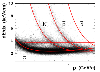
Figure 1: (Color online) $dE/dx$ for negative particles vs. momentum measured by the TPC in Au+Au collisions. The curves are the Bethe-Bloch parametrization pdg for different particle species.

In addition to momentum information, the TPC provides particle identification for charged particles by measuring their ionization energy loss ($dE/dx$). The TPC measurement of $dE/dx$ as a function of the momentum ($p$) is shown in Fig. 1. Different bands seen in Fig. 1 represent Bethe-Bloch distributions pdg folded with the experimental resolutions and correspond to different particle species. Charged pions and kaons can be identified with their momenta up to about 0.75 GeV/$c$ while protons and anti-protons can be identified with momenta up to about 1.1 GeV/$c$. In order to quantitatively describe the particle identification, the variable $N_{\sigma\pi}$ (e.g. pions) was defined as

$$N_{\sigma\pi}=\frac{1}{R}\log\frac{dE/dx_{\text{measured}}}{\langle dE/dx\rangle_{\pi}},$$ (1)

where $dE/dx_{\text{measured}}$ is the measured energy loss for a track, $\langle dE/dx\rangle_{\pi}$ is the expected mean energy loss for charged pions with a given momentum, and $R$ is the $dE/dx$ resolution which varies between 6% and 10% from $p+p$ to central Au+Au events and depends on the characteristics of each track, such as the number of $dE/dx$ hits for a track measured in the TPC, the pseudorapidity of a track, etc. We construct $N_{\sigma K}$ in a similar way for the charged kaon identification. Specific analysis cuts (described later) were then applied on $N_{\sigma\pi}$ and $N_{\sigma K}$ in order to quantitatively select the charged pion and kaon candidate tracks.

III Particle Selections

In this analysis, the hadronic decay channels of $K(892)^{*0}\rightarrow K^{+}\pi^{-}$, $\overline{K(892)^{*0}}\rightarrow K^{-}\pi^{+}$ and $K(892)^{*\pm}\rightarrow K_{S}^{0}\pi^{\pm}$ were measured. In the following, the term $K^{*0}$ stands for $K^{*0}$ or $\overline{K^{*0}}$, and the term $K^{*}$ stands for $K^{*0}$, $\overline{K^{*0}}$ or $K^{*\pm}$, unless otherwise specified.

Table 1: List of track cuts for charged kaon and charged pion and topological cuts for neutral kaon used in the $K^{*}$ analysis in Au+Au and $p+p$ collisions. $decayLength$ is the decay length, $dcaDaughters$ is the distance of closest approach between the daughters, $dcaV0PrmVx$ is the distance of closest approach between the reconstructed $K_{S}^{0}$ momentum vector and the primary interaction vertex, $dcaPosPrmVx$ is the distance of closest approach between the positively charged granddaughter and the primary vertex, $dcaNegPrmVx$ is the distance of closest approach between the negatively charged granddaughter and the primary vertex, $M_{K_{S}^{0}}$ is the $K_{S}^{0}$ invariant mass in GeV/$c^{2}$, $NFitPnts$ is the number of fit points of a track in the TPC, $NTpcHits$ is the number of hits of a track in the TPC, $MaxPnts$ is the number of maximum possible points of a track in the TPC, and $DCA$ is the distance of closest approach to the primary interaction point.

Cuts	$K^{*0}$		$K^{*\pm}$
	Au+Au	$p+p$	Daughter $\pi^{\pm}$	$K_{S}^{0}$
$N_{\sigma K}$	(-2.0, 2.0)	(-2.0, 2.0)		$decayLength>$ 2.0 cm
$N_{\sigma\pi}$	(-3.0, 3.0)	(-2.0, 2.0)	(-2.0, 2.0)	$dcaDaughters<$ 1.0 cm
Kaon $p$ (GeV/$c$)	(0.2, 10.0)	(0.2, 0.7)		$dcaV0PrmVx<$ 1.0 cm
Kaon $p_{T}$ (GeV/$c$)	(0.2, 10.0)	(0.2, 0.7)		$dcaPosPrmVx>$ 0.5 cm
Pion $p$ (GeV/$c$)	(0.2, 10.0)	(0.2, 10.0)	(0.2, 10.0)	$dcaNegPrmVx>$ 0.5 cm
Pion $p_{T}$ (GeV/$c$)	(0.2, 10.0)	(0.2, 10.0)	(0.2, 10.0)	$M_{K_{S}^{0}}$ (GeV/$c^{2}$): (0.48, 0.51)
$NFitPnts$	$>$ 15	$>$ 15	$>$ 15	$\pi^{+}$: $NTpcHits>$ 15
$NFitPnts/MaxPnts$	$>$ 0.55	$>$ 0.55	$>$ 0.55	$\pi^{-}$: $NTpcHits>$ 15
Kaon and pion $\eta$	$|\eta|<$ 0.8	$|\eta|<$ 0.8	$|\eta|<$ 0.8	$\pi^{+}$: $p>$ 0.2 GeV/$c$
$DCA$ (cm)	$<$ 3.0	$<$ 3.0	$<$ 3.0	$\pi^{-}$: $p>$ 0.2 GeV/$c$
Pair ($K\pi$) $y$	$|y|<$ 0.5

Since the $K^{*}$ decays in such short time that the daughters seem to originate from the interaction point, only charged kaon and charged pion candidates whose distance of closest approach to the primary interaction vertex was less than 3 cm were selected. Such candidate tracks are defined as “primary tracks”. The charged $K^{*}$ first undergoes a strong decay to produce a $K_{S}^{0}$ and a charged pion herein labeled as the $K^{*\pm}$ daughter pion. Then, the produced $K_{S}^{0}$ decays weakly into $\pi^{+}\pi^{-}$ with $c\tau$ = 2.67 cm. Two oppositely charged pions from the $K_{S}^{0}$ decay are called as the $K^{*\pm}$ granddaughter pions. The charged daughter pion candidates were selected from primary track samples and the $K_{S}^{0}$ candidates were selected through their decay topology.

In Au+Au collisions, charged kaon candidates were selected by requiring $|N_{\sigma K}|<2$ while a looser cut $|N_{\sigma\pi}|<3$ was applied to select the charged pion candidates to maximize the statistics for the $K^{*0}$ analysis. Such $N_{\sigma}$ cuts can only ambiguously select the kaons and pions if applied to the tracks with their momenta beyond the momentum range specified earlier. However, these cuts help to significantly reduce the background. In order to avoid the acceptance drop in the high $\eta$ range, all kaon and pion candidates were required to have $|\eta|<$ 0.8. Kaon and pion candidates were also required to have at least 15 fit points (number of measured TPC hits used in track fit, maximum 45 fit points) to assure track fitting quality and good $dE/dx$ resolution. For all the track candidates, the ratio between the number of TPC track fit points over the maximum possible points was required to be greater than 0.55 to avoid selecting split tracks. To maintain reasonable momentum resolution, only tracks with $p_{T}$ larger than 0.2 GeV/$c$ were selected.

In $p+p$ collisions, enough data were available to precisely measure the $K^{*0}$ mass, width, and invariant yield as a function of $p_{T}$. As statistics was not an issue for this analysis, only kaon candidates with $p<0.7$ GeV/$c$ were used to ensure clean identification. This kaon momentum cut helped minimize contamination from misidentified correlated pairs and thus reduce the systematic uncertainty. In the case of the pion candidates, the same $p$ and $p_{T}$ cuts as used in Au+Au collisions were applied. Charged kaon and pion candidates were selected by requiring $|N_{\sigma\pi,K}|<2$ to reduce the residual background. All other track cuts for both kaon and pion candidates were the same as for Au+Au data.

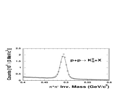
Figure 2: $K_{S}^{0}$ signal observed in the $\pi^{+}\pi^{-}$ invariant mass distribution reconstructed from the decay topology method via $K_{S}^{0}\rightarrow\pi^{+}\pi^{-}$ in $p+p$ collisions. The dashed curve depicts the Gaussian fit function plus a linear function representing the background.

The $K^{*\pm}$ was measured only in minimum bias $p+p$ interactions and in peripheral 50-80% Au+Au collisions. Daughter pions for the $K^{*\pm}$ reconstruction were required to originate from the interaction point and pass the same cuts as used for the $K^{*0}$ analysis in $p+p$ collisions. The $K_{S}^{0}$ was reconstructed by the decay topology method kshort ; lambda1 . The granddaughter charged pion candidates were selected from global tracks (tracks do not necessarily originate from the primary collision vertex) with a distance of closest approach to the interaction point greater than 0.5 cm. Candidates for the granddaughter charged pions were also required to have at least 15 hit points in the TPC with $p>$ 0.2 GeV/$c$. Oppositely charged candidates were then paired to form neutral decay vertices. The distance of closest approach for each pair was required to be less than 1.0 cm and the neutral decay vertices were required to be at least 2.0 cm away from the primary vertex to reduce the combinatorial background. The reconstructed $K_{S}^{0}$ momentum vector was required to point back to the primary interaction point within 1.0 cm. Only the $K_{S}^{0}$ candidates with $\pi^{+}\pi^{-}$ invariant mass between 0.48 and 0.51 GeV/$c^{2}$ were selected. When the $K_{S}^{0}$ candidate was paired with the daughter pion to reconstruct the charged $K^{*}$, tracks were checked to avoid double-counting among the three tracks used. Fig. 2 shows the $K_{S}^{0}$ signal observed in the $\pi^{+}\pi^{-}$ invariant mass distribution in $p+p$ collisions. The Gaussian width of the above $K_{S}^{0}$ signal is around 7 MeV/$c^{2}$ which is mainly determined by the momentum resolution of the detector. Due to detector effects, such as the daughter tracks’ energy loss in the TPC, etc., the $K_{S}^{0}$ mass is shifted by $-$3 MeV/c². The measured $K_{S}^{0}$ mass and width agree well with Monte Carlo ($MC$) simulations, which included the finite momentum resolution of the detector and the daughter tracks’ energy loss in the TPC.

The $K\pi$ pairs with their parent rapidity ($y$) of $|y|<0.5$ were selected. All the cuts used in this $K^{*}$ analysis are summarized in Table 1. After all the above mentioned cuts have been applied, the $K^{*}$ reconstruction efficiencies multiplied by the detector acceptance are shown in Fig. 9.

IV Extraction of the $K^{*}$ Signal

In Au+Au collisions, up to several thousand charged tracks per event originate from the primary collision vertex. The daughters from $K^{*}$ decays are topologically indistinguishable from other primary particles. The measurement was performed by calculating the invariant mass for each $K\pi$ pair in an event. The $K^{\pm}\pi^{\mp}$ invariant mass distribution is shown in Fig. 3 as open circles. The unlike-sign $K\pi$ invariant mass distribution derived in this manner was mostly from random $K\pi$ combinatorial pairs. The signal to background is between 1/200 for minimum bias Au+Au and 1/10 for minimum bias $p+p$. The overwhelming combinatorial background distribution can be obtained and subtracted from the unlike-sign $K\pi$ invariant mass distribution in two ways:

• the mixed-event technique: reference background distribution is built with uncorrelated unlike-sign kaons and pions from different events;

• the like-sign technique: reference background distribution is made from like-sign kaons and pions in the same event.

The mixed-event technique has been successfully used in the measurement of resonances at RHIC, such as the $K(892)^{*0}$ in Au+Au collisions at $\sqrt{s_{{}_{NN}}}=$ 130 GeV kstar130 and the $\phi$ in Au+Au collisions at $\sqrt{s_{{}_{NN}}}=$ 130 and 200 GeV phi1 ; phi2 . This technique was also used in the measurement of $\Lambda$ production in Au+Au collisions at $\sqrt{s_{{}_{NN}}}$ = 130 GeV, and the results agree well with those from the decay topology method lambda1 ; lambda2 . The like-sign technique has been successfully applied in measuring $\rho(770)^{0}\rightarrow\pi^{+}\pi^{-}$ production in $p+p$ and peripheral Au+Au collisions at $\sqrt{s_{{}_{NN}}}=$ 200 GeV at RHIC rho1 .

IV.1 Mixed-Event Technique

In order to subtract the uncorrelated pairs from the unlike-sign $K\pi$ invariant mass distribution obtained from the same events, an unlike-sign $K\pi$ invariant mass spectrum from mixed events was obtained. In order to keep the event characteristics as similar as possible among different events, the whole data sample was divided into 10 bins in charged particle multiplicity and 10 bins in the collision vertex position along the beam direction. Only pairs from events in the same multiplicity and vertex position bins were selected.

Figure 3: The unlike-sign $K\pi$ invariant mass distribution (open symbols) and the mixed-event $K\pi$ invariant mass distribution after normalization (solid curve) from minimum bias Au+Au collisions.

In the unlike-sign invariant mass distribution from an event, $K^{+}_{1}\pi^{-}_{1}$ and $K^{-}_{1}\pi^{+}_{1}$ pairs were sampled which include the desired $K^{*}$ signal and the background. In the mixed-event spectrum, $K^{+}_{1}\pi^{-}_{i}$ , $K^{-}_{1}\pi^{+}_{i}$, $K^{+}_{i}\pi^{-}_{1}$, and $K^{-}_{i}\pi^{+}_{1}$ pairs were sampled for the background estimation. The subscripts 1 and $i$ correspond to event numbers with $i\neq$1. The number of events to be mixed was chosen to be 5, so that the total number of entries in the mixed-event invariant mass distribution was $\sim$10 times that of the total number of entries in the distribution from the same events. Thus the mixed-event spectrum needs to be normalized in order to subtract the background in the unlike-sign spectrum. Since the $K\pi$ pairs with invariant mass greater than 1.1 GeV/$c^{2}$ are less likely to be correlated in the unlike-sign distribution, the normalization factor was calculated by taking the ratio between the number of entries in the unlike-sign and the mixed-event distributions for invariant mass greater than 1.1 GeV/$c^{2}$. The solid curve in Fig. 3 corresponds to the mixed-event $K\pi$ pair invariant mass distribution after normalization. The mixed-event distribution was then subtracted from the unlike-sign distribution as follows:

$$N_{K^{*0}}(m)=N_{K^{+}_{1}\pi^{-}_{1}}(m)+N_{K^{-}_{1}\pi^{+}_{1}}(m)$$

$$-R\times\sum_{i=2}^{6}[N_{K^{+}_{1}\pi^{-}_{i}}(m)+N_{K^{-}_{1}\pi^{+}_{i}}(m)$$

$$+N_{K^{+}_{i}\pi^{-}_{1}}(m)+N_{K^{-}_{i}\pi^{+}_{1}}(m)],$$ (2)

where $N$ is the number of entries in a bin with its center at the $K\pi$ pair invariant mass $m$ and $R$ is the normalization factor. After the mixed-event background subtraction, the $K^{*0}$ signal is visible as depicted by the open star symbols in Fig. 5.

IV.2 Like-Sign Technique

The like-sign technique is another approach to subtract the background of non-correlated pairs from the unlike-sign $K\pi$ invariant mass distribution from the same events. The uncorrelated background in the unlike-sign $K\pi$ distribution was described by using the invariant mass distributions obtained from uncorrelated $K^{+}\pi^{+}$ and $K^{-}\pi^{-}$ pairs from the same events.

In the unlike-sign $K\pi$ invariant mass spectrum, $K^{+}_{1}\pi^{-}_{1}$ and $K^{-}_{1}\pi^{+}_{1}$ pairs were sampled. $K^{+}_{1}\pi^{+}_{1}$ and $K^{-}_{1}\pi^{-}_{1}$ pairs were sampled in the like-sign $K\pi$ invariant mass distribution. Since the number of positive and negative particles may not be the same in relativistic heavy-ion collisions, in order to correctly subtract the subset of non-correlated pairs in the unlike-sign $K\pi$ distribution, the like-sign $K\pi$ invariant mass distribution was calculated as follows:

$$N_{\text{Like-Sign}}(m)=2\times\sqrt{N_{K^{+}_{1}\pi^{+}_{1}}(m)\times N_{K^{-}_{1}\pi^{-}_{1}}(m)},$$ (3)

where $N$ is the number of entries in a bin with its center at the $K\pi$ pair invariant mass $m$. The unlike-sign and the like-sign invariant mass distributions are shown in Fig. 4. The like-sign spectrum was then subtracted from the unlike-sign distribution:

$$N_{K^{*0}}(m)=N_{K^{+}_{1}\pi^{-}_{1}}(m)+N_{K^{-}_{1}\pi^{+}_{1}}(m)-N_{\text{Like-Sign}}(m).$$ (4)

The like-sign background subtracted $K\pi$ invariant mass distribution corresponds to the solid square symbols in Fig. 5, where the $K^{*0}$ signal is now visible.

Compared to the mixed-event technique, the like-sign technique has the advantage that the unlike-sign and like-sign pairs are taken from the same event, so there is no event structure difference between the two distributions due to effects such as elliptic flow. The short-coming of this technique is that the like-sign distribution has larger statistical uncertainties compared to the mixed-event spectrum, since the statistics in the mixed-event and like-sign techniques are driven by the number of events mixed and the number of kaons and pions produced per event, respectively haibin . Therefore, in this analysis, the mixed-event technique was used to reconstruct the $K^{*}$ signal whereas the like-sign technique was used to study the sources of the residual background under the $K^{*0}$ peak after mixed-event background subtraction as discussed in details in the following text.

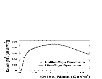
Figure 4: The unlike-sign $K\pi$ invariant mass distribution (open symbols) and the like-sign $K\pi$ invariant mass distribution (solid curve) from minimum bias Au+Au collisions.

IV.3 Describing the Residual Background

The unlike-sign $K\pi$ invariant mass distribution after mixed-event background subtraction is represented by the open star symbols in Fig. 5, where the $K^{*0}$ signal is clearly observed. The mixed-event technique removes only the uncorrelated background pairs in the unlike-sign spectrum. As a consequence, residual correlations near the $K^{*0}$ mass range were not subtracted by the mixed-event spectrum. This residual background may come from three dominant sources:

• elliptic flow in non-central Au+Au collisions;

• correlated real $K\pi$ pairs;

• correlated but misidentified pairs.

The overlapping region of non-central Au+Au collisions has an elliptic shape in the plane perpendicular to the beam axis. Each non-central Au+Au event has a unique reaction plane angle. The azimuthal distributions for kaons and pions may be different for different events. Thus, the unlike-sign $K\pi$ pair invariant mass spectrum may have a different structure than the mixed-event invariant mass distribution. This structural difference may lead to a significant residual background in the unlike-sign $K\pi$ invariant mass spectrum after mixed-event background subtraction gaudichet .

In the like-sign technique, the unlike-sign $K\pi$ spectrum and the like-sign distribution are obtained from the same events. Therefore, no correlations due to elliptic flow should be present in the unlike-sign $K\pi$ invariant mass spectrum after like-sign background subtraction. In Fig. 5, the solid square symbols represent the unlike-sign $K\pi$ invariant mass distribution after like-sign background subtraction. The amplitude of the residual background below the peak after the like-sign background subtraction is about a factor of 2 smaller than after the mixed-event background subtraction, while the amplitude of the $K^{*0}$ signal remains the same. This indicates that part of the residual background in the spectrum after mixed-event background subtraction was induced by elliptic azimuthal anisotropy.

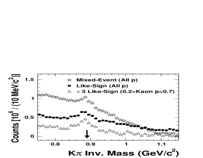
Figure 5: The $K\pi$ invariant mass distributions after event-mixing background subtraction (open star symbols) and like-sign background subtraction with different daughter momentum cuts (0.2 $<$ Kaon and Pion $p<$ 10 GeV/$c$ for filled square symbols, 0.2 $<$ Kaon $p<$ 0.7 GeV/$c$ and 0.2 $<$ Pion $p<$ 10 GeV/$c$ for open triangle symbols) demonstrating the sources of the residual background in minimum bias Au+Au collisions. The open triangle symbols have been scaled up by a factor of 3 in order to increase the visibility. The arrow depicts the standard $K^{*0}$ mass of 896.1 MeV/$c^{2}$ pdg .

In the $K^{*0}$ analysis in Au+Au collisions, since the kaons and pions are selected with 0.2 $<p<$ 10.0 GeV/$c$, a pion (kaon) with $p>$ 0.75 GeV/$c$ may be misidentified as a kaon (pion). A proton with $p>$ 1.1 GeV/$c$ may be misidentified as either a kaon or a pion, or both, depending on whether kaons or pions are being selected. Electrons and positrons which cross the kaon (pion) band in the $dE/dx$ plot shown in Fig. 1 may be misidentifed as kaons (pions). Thus, the daughters from $\rho^{0}\rightarrow\pi^{+}\pi^{-}$, $\phi\rightarrow K^{+}K^{-}$, $\Lambda\rightarrow\pi^{-}p$, etc. could be falsely identified as a $K\pi$ pair if the daughter momenta are beyond the particle identification range. The invariant mass calculated from these misidentified pairs cannot be subtracted away by the mixed-event background and remains as part of the residual background.

In Fig. 5, the open triangle symbols correspond to the unlike-sign $K\pi$ spectrum after like-sign background subtraction with 0.2 $<p<$ 0.7 GeV/$c$ and 0.2 $<p<$ 10.0 GeV/$c$ for the kaon and the pion, respectively. These momentum cuts allow only correlated $K\pi$ real pairs and pairs in which a kaon or a proton was misidentified as a pion to contribute to the background subtracted spectrum. Compared to the solid square symbols in Fig. 5, the residual background represented by the open triangle symbols is reduced by a factor of 6 and the $K^{*0}$ signal is a factor of 2 smaller. This indicates that particle misidentification of the decay products of $\rho$, $\omega$, $\eta$, $K_{S}^{0}$, $\Lambda$, etc. indeed causes false correlations to appear in the background subtracted distribution.

Correlated real $K\pi$ pairs from real particle decays, such as higher mass resonant states in the $K-\pi$ system and particle decay modes with three or more daughters where two of them are a $K\pi$ pair, as well as the nonresonant $K-\pi$ $s$-wave correlation also contribute to the unlike-sign $K\pi$ spectrum. These correlated $K\pi$ pairs contribute to the residual background, since they are not present in the like-sign and mixed-event distributions. There is no efficient cut to remove these real correlations from the residual background.

V Analysis and Results

V.1 $K^{*0}$ Mass and Width

Figure 6 depicts the mixed-event background subtracted $K\pi$ invariant mass distributions ($M_{K\pi}$) integrated over the $K^{*}$ $p_{T}$ for central Au+Au (upper panel) and for minimum bias $p+p$ (lower panel) interactions. The mass of the $K^{*0}$ was fit to the function:

$$BW\times PS+RBG,$$ (5)

where $BW$ is the relativistic $p$-wave Breit-Wigner function upc :

$$BW=\frac{M_{K\pi}\Gamma M_{0}}{(M_{K\pi}^{2}-M_{0}^{2})^{2}+M_{0}^{2}\Gamma^{2}},$$ (6)

$PS$ is the Boltzmann factor rapp4 ; shuryak ; pbm1 ; kolb :

$$PS=\frac{M_{K\pi}}{\sqrt{M_{K\pi}^{2}+p_{T}^{2}}}\times\exp\left(-\frac{\sqrt{M_{K\pi}^{2}+p_{T}^{2}}}{T_{fo}}\right)$$ (7)

that accounts for phase space, and $RBG$ is the linear function:

$$RBG=a+bM_{K\pi}.$$ (8)

that represents the residual background. Within this parametrization, $T_{fo}$ is the temperature at which the resonance is emitted shuryak and

$$\Gamma=\frac{\Gamma_{0}M_{0}^{4}}{M_{K\pi}^{4}}\times\left[\frac{(M_{K\pi}^{2}-M_{\pi}^{2}-M_{K}^{2})^{2}-4M_{\pi}^{2}M_{K}^{2}}{(M_{0}^{2}-M_{\pi}^{2}-M_{K}^{2})^{2}-4M_{\pi}^{2}M_{K}^{2}}\right]^{3/2}$$ (9)

is the momentum dependent width upc . In addition, $M_{0}$ is the $K^{*}$ mass, $\Gamma_{0}$ is the $K^{*}$ width, $p_{T}$ is the $K^{*}$ transverse momentum, $M_{\pi}$ is the pion mass, and $M_{K}$ is the kaon mass.

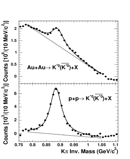
Figure 6: The $K\pi$ invariant mass distribution integrated over the $K^{*}$ $p_{T}$ for central Au+Au (upper panel) and minimum bias $p+p$ (lower panel) interactions after the mixed-event background subtraction. The solid curves are the fits to Eq. 5 with $T_{fo}$ = 120 MeV and $p_{T}$ = 1.8 GeV/$c$ for central Au+Au and $T_{fo}$ = 160 MeV and $p_{T}$ = 0.8 GeV/$c$ for $p+p$, respectively. The dashed lines are the linear function representing the residual background.

The $PS$ factor accounts for $K^{*}$ produced through kaon and pion scattering, or $K+\pi\rightarrow K^{*}\rightarrow K+\pi$. In Au+Au collisions, the thermal freeze-out temperature $T_{fo}$ = 90 MeV was measured at STAR meanpt . However, resonances can be produced over a range of temperature inside the hadronic system and not all resonances are emitted at the point where the system freezes out at $T_{fo}$ = 90 MeV. As a result, the temperature chosen in the PS factor was 120 MeV according to shuryak . The temperature of $T_{fo}$ = 90 MeV was also used to estimate the systematic uncertainties which are about 1.5 MeV/$c^{2}$ for masses and 5 MeV/$c^{2}$ due the choice of $T_{fo}$. In $p+p$ collisions, particle production is well reproduced by the statistical model becattini with $T_{fo}$ = 160 MeV and therefore this was the temperature used in the $PS$ factor. $p_{T}$ = 1.8 GeV/$c$ and 0.8 GeV/$c$ were chosen in the $PS$ factor for the Au+Au and $p+p$ collisions respectively which are the centers of the entire measured $p_{T}$ ranges (0.4 $<p_{T}<$ 3.2 GeV/$c$ for Au+Au and $p_{T}<$1.6 GeV/$c$ for p+p).

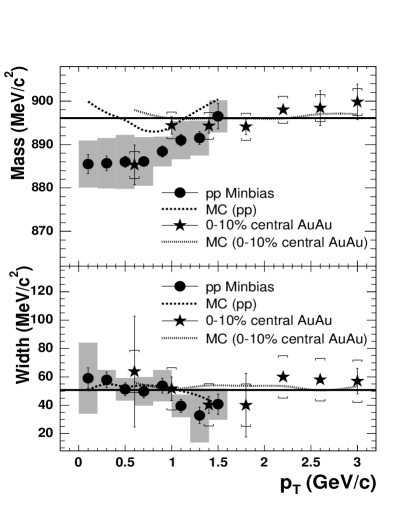
Figure 7: The $K^{*0}$ mass (upper panel) and width (lower panel) as a function of $p_{T}$ for minimum bias $p+p$ interactions and for central Au+Au collisions. The solid straight lines are the standard $K^{*0}$ mass (896.1 MeV/$c^{2}$) and width (50.7 MeV/c²) pdg , respectively. The dashed and dotted curves are the $MC$ results in minimum bias $p+p$ and for central Au+Au collisions, respectively, after considering detector effects and kinematic cuts. The grey shadows (caps) indicate the systematic uncertainties for the measurement in minimum bias $p+p$ interactions (central Au+Au collisions).

Mixed-event background subtracted $K\pi$ invariant mass distributions were obtained for different $p_{T}$ bins, and each $p_{T}$ bin was fit to Eq. 5 with the $K^{*0}$ mass, width, and uncorrected yield as free parameters. The $\chi^{2}/ndf$ of the fit varies between 0.6 and 1.7 for all $p_{T}$ bins except for two $p_{T}$ bins (3.8 for the $2.0<p_{T}<2.4$ GeV/$c$ bin and 2.6 for the $2.4<p_{T}<2.8$ GeV/$c$ bin) in the central Au+Au data, where the uncertainties of the mass and width values are not well constrained. Figure 7 shows the $K^{*0}$ mass (upper panel) and width (lower panel) for central Au+Au and for minimum bias $p+p$ interactions as a function of the $K^{*0}$ $p_{T}$. $MC$ calculations for the $K^{*0}$ mass and width were obtained by simulating $K^{*0}$ with standard mass and width values pdg and passing them through the same reconstruction steps and kinematic cuts as the real data. The results from such simulations are also depicted in Fig. 7. The deviations between the $MC$ results and the standard mass and width values are mainly due to the kinematic cuts (track $p$ and $p_{T}$ cuts, etc.). For example, the $p_{T}>0.2$ GeV/$c$ cut results in the rise of the mass at low $p_{T}$ and the kaon $p<0.7$ GeV/$c$ cut in $p+p$ causes the rise of the mass and the drop of the width at higher $p_{T}$. Our $MC$ studies indicate that the deviations induced by kinematic cuts are not sufficient to explain the mass shift seen in the data.

The systematic uncertainties in the $K^{*0}$ mass and width for the measurement in minimum bias $p+p$ interactions were evaluated bin-by-bin by varying the particle types (either $K^{*0}$ or $\overline{K^{*0}}$ ), the methods in the background subtraction (mixed-event or like-sign), the residual background functions (exponential or second order polynomial functions), the dynamical cuts, the track types (primary tracks or global tracks), and by considering the detector effects (different TPC magnetic field directions, different sides of the TPC detector, etc.). Due to the limited statistics, the systematic uncertainties (3.1 MeV/c² for masses and 14.9 MeV/c² for widths) in central Au+Au interactions were only estimated using the entire measured $p_{T}$ range ($0.4<p_{T}<3.2$ GeV/$c$) following the above steps. More detailed discussions about the systematic uncertainty studies can be found in haibin . In minimum bias p+p interactions, the $K^{*0}$ masses at low $p_{T}$ (first 2-3 data points) are lower than the $MC$ results at a 2-3$\sigma$ level.

V.2 $m_{T}$ and $p_{T}$ Spectra

Mixed-event background subtracted $K\pi$ invariant mass distributions were obtained for different $p_{T}$ bins, and each $p_{T}$ bin was fit to function:

$$SBW+RBG,$$ (10)

where $SBW$ is the non-relativistic Breit-Wigner function pdg :

$$SBW=\frac{\Gamma_{0}}{(M_{K\pi}-M_{0})^{2}+\Gamma_{0}^{2}/4}$$ (11)

and $RBG$ is the linear function from Eq. 8 that represents the residual background. The fit sensitivity to statistical fluctuations in the $K^{*}$ raw yield was reduced by fixing the mass and width in the fit according to the values obtained from the free parameter fit with the same simplified $BW$ function. The $\chi^{2}/ndf$ of the fit varies between 0.7 and 1.8 for all $p_{T}$ bins except for two $p_{T}$ bins ($\sim$3.0 for the $2.0<p_{T}<2.4$ GeV/$c$ bin and $\sim$2.7 for the $2.4<p_{T}<2.8$ GeV/$c$ bin) in Au+Au data. The $K^{*}$ raw yield was also obtained by fitting the data to the $BW$ function from Eq. 6 with all parameters free in the fit. The difference in the raw yields between the two fit functions was included in the systematic uncertainties. The $K_{S}^{0}\pi^{\pm}$ invariant mass distribution fit to Eq. 10 after the mixed-event background subtraction is shown in Fig. 8 for minimum bias $p+p$ collisions (upper panel) and for the 50-80% of the inelastic hadronic Au+Au cross-section (lower panel).

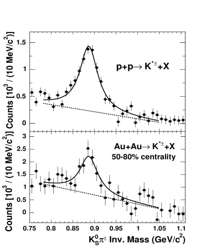
Figure 8: The $K_{S}^{0}\pi^{\pm}$ invariant mass distribution integrated over the $K^{*\pm}$ $p_{T}$ for minimum bias $p+p$ collisions (upper panel) and for the 50-80% of the inelastic hadronic Au+Au cross-section (lower panel) after the mixed-event background subtraction. The solid curves are fits to Eq. 10 and the dashed lines are the linear function representing the residual background.

About 6$\times$10⁶, 2$\times$10⁶ and 5.6$\times$10⁴ $K^{*0}$ signals were reconstructed from top 10% central Au+Au, minimum bias Au+Au and minimum bias $p+p$ collisions respectively while about 1.2$\times$10⁴ and 10⁴ $K^{*\pm}$ were observed in the 50-80% Au+Au and minimum bias $p+p$ collisions respectively. The $K^{*0}$ and $K^{*\pm}$ raw yields obtained for different $p_{T}$ bins in Au+Au and minimum bias $p+p$ collisions were then corrected for the detector acceptance and efficiency (shown in Fig. 9) determined from a detailed simulation of the TPC response using GEANT hminus . The corresponding branching ratios were also taken into account. In addition, the yields in $p+p$ were corrected for the collision vertex finding efficiency of 86%.

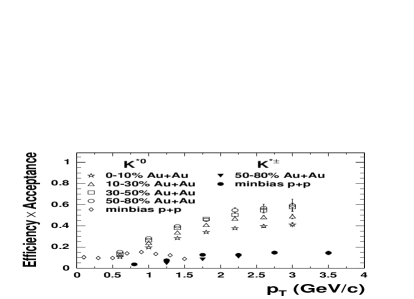
Figure 9: The $K^{*0}$ and $K^{*\pm}$ reconstruction efficiency multiplied by the detector acceptance as a function of $p_{T}$ in minimum bias $p+p$ and different centralities in Au+Au collisions.

The transverse mass ($m_{T}$) distributions of the midrapidity $(K^{*0}+\overline{K^{*0}})/2$ invariant yields in central Au+Au, four different centralities in minimum bias Au+Au, and minimum bias $p+p$ collisions are depicted in Fig. 10. The $(K^{*+}+K^{*-})/2$ invariant yields for the most peripheral 50-80% Au+Au collisions are also shown for comparison. The $K^{*0}$ invariant yield [$d^{2}N/(2\pi m_{T}dydm_{T})$] distributions were fit to an exponential function:

$$\frac{1}{2\pi m_{T}}\frac{d^{2}N}{dydm_{T}}=\frac{dN}{dy}\frac{1}{2\pi T(m_{0}+T)}$$

$$\exp\left(\frac{-(m_{T}-m_{0})}{T}\right),$$ (12)

where $dN/dy$ is the $K^{*0}$ yield at $|y|<0.5$ and $T$ is the inverse slope parameter. The extracted $dN/dy$ and $T$ parameters are listed in Table 2. The systematic uncertainties on the $K^{*0}$ $dN/dy$ and $T$ in Au+Au and $p+p$ collisions were estimated by comparing different Breit-Wigner functions, particle types (either $K^{*0}$ or $\overline{K^{*0}}$), residual background functions (exponential or second order polynomial functions), dynamical cuts, and by considering the detector effects. More detailed discussions about the systematic uncertainty studies can be found in haibin . The $K^{*0}$ invariant yield increases from $p+p$ collisions to peripheral Au+Au and to central Au+Au collisions. The inverse slope of the $K^{*0}$ spectra for all centrality bins of Au+Au collisions is significantly larger than in minimum bias $p+p$ collisions.

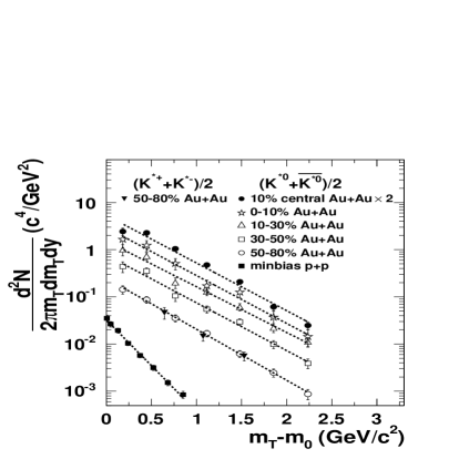
Figure 10: The ($K^{*}+\overline{K^{*}}$)/2 invariant yields as a function of $m_{T}-m_{0}$ for $|y|<$ 0.5 from minimum bias $p+p$ and different centralities in Au+Au collisions. The top 10% central data have been multiplied by two for clarity. The lines are fits to Eq. 12. The errors shown are the quadratic sum of statistical and systematic (in the level of 10%) uncertainties.

Table 2: The $K^{*0}$ $dN/dy$ and $T$ for $|y|<$ 0.5 from central Au+Au, four different centralities in minimum bias Au+Au, and minimum bias $p+p$ collisions. The first error is statistical, the second is systematic.

	$dN/dy$	$T$ (MeV)
top 10% central	10.18$\pm$0.46$\pm$1.88	427$\pm$10$\pm$46
0-10%	10.48$\pm$1.45$\pm$1.94	428$\pm$31$\pm$47
10-30%	5.86$\pm$0.56$\pm$1.08	446$\pm$23$\pm$49
30-50%	2.81$\pm$0.25$\pm$0.52	427$\pm$18$\pm$46
50-80%	0.82$\pm$0.06$\pm$0.15	402$\pm$14$\pm$44
$p+p$	(5.08$\pm$0.17$\pm 0.61$)$\times$10-2	223$\pm$8$\pm$9

Theoretical calculations powerlaw indicate that in $p+p$ collisions, particle production is dominated by hard processes for $p_{T}$ above 1.5 GeV/$c$ while soft processes dominate at low $p_{T}$. Thus in the $K^{*}$ $p_{T}$ spectrum, a power-law shape for $p_{T}$ above 1.5 GeV/$c$ and an exponential shape at lower $p_{T}$ should be expected. In minimum bias $p+p$ collisions, due to the cut on the kaon daughter of $p<0.7$ GeV/$c$, only the $K^{*0}$ spectrum for $p_{T}<1.6$ GeV/$c$ was measured. As a result, the $K^{*0}$ $m_{T}$ spectrum in minimum bias $p+p$ collisions can be well described by the commonly used exponential function, as shown in Fig. 10. The $K^{*}$ $p_{T}$ spectrum can be extended to higher $p_{T}$ by measuring the $K^{*\pm}$ signals. Figure 11 shows the $(K^{*0}+\overline{K^{*0}})/2$ and $(K^{*+}+K^{*-})/2$ invariant yields for $|y|<$ 0.5 as a function of $p_{T}$. The dotted curve in this figure is the fit to the power-law function:

$$\frac{1}{2\pi p_{T}}\frac{d^{2}N}{dydp_{T}}=\frac{dN}{dy}\frac{2(n-1)(n-2)}{\pi(n-3)^{2}\langle p_{T}\rangle^{2}}$$

$$\left(1+\frac{p_{T}}{\langle p_{T}\rangle(n-3)/2}\right)^{-n},$$ (13)

where $n$ is the order of the power law and $\langle p_{T}\rangle$ is the average transverse momentum. The data were fit for $p_{T}>0.5$ GeV/$c$. The power-law fit does not reproduce the two first $p_{T}$ bins (0.0 $\leq p_{T}<$ 0.2 GeV/$c$ and 0.2 $\leq p_{T}<$ 0.4 GeV/$c$) since at low $p_{T}$ particle production may be dominated by soft processes. From the power-law fit, the $\chi^{2}/ndf$ is 0.93. The dashed curve in Fig. 11 is the $K^{*0}$ spectrum fit to the exponential function from Eq. 12 and then extrapolated to higher $p_{T}$. The data could not be described by this exponential fit indicating that hard processes dominate the particle production for $p_{T}>1.5$ GeV/$c$. Some model levy1 suggests to use the Levy function in Equation 14 to represent the $p_{T}$ spectrum:

$$\frac{1}{2\pi p_{T}}\frac{d^{2}N}{dydp_{T}}=\frac{dN}{dy}\frac{(n-1)(n-2)}{2\pi nT(nT+m_{0}(n-2))}$$

$$\left(1+\frac{\sqrt{p_{T}^{2}+m_{0}^{2}}-m_{0}}{nT}\right)^{-n}.$$ (14)

The dashed-dotted curve in Fig. 11 is the Levy function fit with $\chi^{2}/ndf=$ 0.90 to the $K^{*}$ spectrum in all the measured $p_{T}$ range ($p_{T}<4$ GeV/$c$).

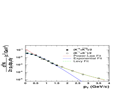
Figure 11: (Color online) The invariant yields for both ($K^{*0}+\overline{K^{*0}}$)/2 and ($K^{*+}+K^{*-}$)/2 as a function of $p_{T}$ for $|y|<$ 0.5 in minimum bias $p+p$ interactions. The dotted curve is the fit to the power-law function from Equation 13 for $p_{T}>0.5$ GeV/$c$ and extended to lower values of $p_{T}$. The dashed curve is the $K^{*0}$ spectrum fit to the exponential function from Equation 12 and extended to higher values of $p_{T}$. The dashed-dotted curve is the fit to the Levy function from Equation 14 for $p_{T}<4$ GeV/$c$. Errors are statistical only.

V.3 Average Transverse Momentum $\langle p_{T}\rangle$

In Au+Au collisions, the $p_{T}$ range of the exponential fit covers $>$85% of all the $K^{*}$ yield so that the $K^{*}$ average transverse momentum ($\langle p_{T}\rangle$) can be reasonably calculated by using the inverse slope parameter ($T$) extracted from the exponential fit function and assuming the exponential behavior over all the $p_{T}$ range:

$$\langle p_{T}\rangle=\frac{\int^{\infty}_{0}p_{T}^{2}e^{-(\sqrt{p_{T}^{2}+m_{0}^{2}}-m_{0})/T}dp_{T}}{\int^{\infty}_{0}p_{T}e^{-(\sqrt{p_{T}^{2}+m_{0}^{2}}-m_{0})/T}dp_{T}}.$$

In $p+p$ collisions, the neutral and charged $K^{*}$ spectrum shown in Fig. 11 covers $>$98% of all the $K^{*}$ yield so that the $\langle p_{T}\rangle$ is directly calculated from the data points in the spectrum. The systematic uncertainty in $p+p$ includes the differences between this calculation and the exponential fit to the $K^{*0}$ only at $p_{T}<1.6$ GeV/$c$, the power-law fit to both neutral and charged $K^{*}$ at $p_{T}>1.5$ GeV/$c$, the Levy function fit at $p_{T}<4$ GeV/c. The systematic uncertainties for all the $\langle p_{T}\rangle$ values include the effects discussed in the previous section and the differences caused by different fit functions to the invariant yield, such as the Boltzmann fit ($m_{T}e^{-(m_{T}-m_{0})/T}$) and the blast wave model fit blastwave . The calculated $K^{*}$ $\langle p_{T}\rangle$ for different centralities in Au+Au and minimum bias $p+p$ collisions are listed in Table 3.

Table 3: The $K^{*}$ $\langle p_{T}\rangle$ for different centralities in Au+Au and minimum bias $p+p$ collisions. The first error is statistical, the second is systematic.

	$\langle p_{T}\rangle$ (GeV/$c$)
top 10% central	1.08$\pm$0.03$\pm$0.12
0-10%	1.08$\pm$0.08$\pm$0.12
10-30%	1.12$\pm$0.06$\pm$0.13
30-50%	1.08$\pm$0.05$\pm$0.12
50-80%	1.03$\pm$0.04$\pm$0.12
$p+p$	0.81$\pm$0.02$\pm$0.14

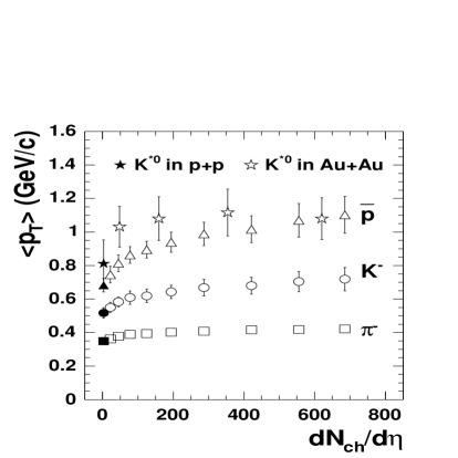
Figure 12: The $K^{*}$ $\langle p_{T}\rangle$ as a function of $dN_{ch}/d\eta$ compared to that of $\pi^{-}$, $K^{-}$, and $\overline{p}$ for minimum bias $p+p$ (solid symbols) and Au+Au (open symbols) collisions. The errors shown are the quadratic sum of the statistical and systematic uncertainties.

The $K^{*}$ $\langle p_{T}\rangle$ as a function of the charged particle multiplicity ($dN_{ch}/d\eta$) is shown in Fig. 12 and compared to that of $\pi^{-}$, $K^{-}$, and $\overline{p}$ meanpt for different centralities in Au+Au and minimum bias $p+p$ collisions. The $K^{*0}$ $\langle p_{T}\rangle$ in Au+Au collisions is significantly larger than in minimum bias $p+p$ collisions. No significant centrality dependence of $\langle p_{T}\rangle$ is observed for $K^{*}$ in Au+Au collisions.

V.4 Particle Ratios

The $K^{*}$ vector meson and its corresponding ground state, the $K$, have identical quark content in the context of the standard model of particles. They differ only in their masses and the relative orientation of their quark spins. Thus, the $K^{*}/K$ yield ratio may be the most interesting and the least model dependent ratio for studying the $K^{*}$ production properties and the freeze-out conditions in relativistic heavy-ion collisions. The $K^{*}$ and $\phi$ mesons have a very small mass difference, their total spin difference is $\Delta S=0$, and both are vector mesons. One significant difference between the $K^{*}$ and $\phi$ is their lifetimes, with the $\phi$ meson lifetime being a factor of 10 longer than that of the $K^{*}$. Therefore, it is important to measure the $\phi/K^{*}$ yield ratio and compare the potential differences in $K^{*}/K$ and $\phi/K$ yield ratios in relativistic heavy-ion collisions to study different hadronic interaction effects on different resonances.

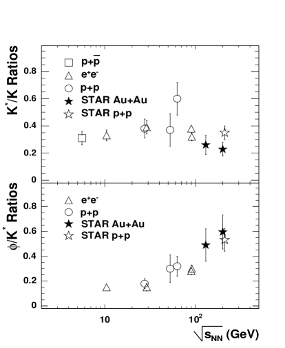
Figure 13: The $K^{*}/K$ (upper panel) and $\phi/K^{*}$ (lower panel) yield ratios as a function of the c.m. system energies. The yield ratios for central Au+Au collisions at $\sqrt{s_{{}_{NN}}}=$ 130 kstar130 and 200 GeV and minimum bias $p+p$ interactions at $\sqrt{s_{{}_{NN}}}=$ 200 GeV are compared to measurements from e⁺e^- at $\sqrt{s}$ of 10.45 GeV alb , 29 GeV der and 91 GeV abe ; pei , $\bar{p}p$ at $\sqrt{s}$ of 5.6 GeV can and $pp$ at $\sqrt{s}$ of 27.5 GeV agu , 52.5 GeV dri and 63 GeV ake . The errors at $\sqrt{s_{NN}}$= 130 and 200 GeV correspond to the quadratic sum of the statistical and systematic errors.

The $K^{*}/K$ yield ratios as a function of the c.m. system energies are shown in the upper panel of Fig. 13. The $K^{*}/K^{-}$ yield ratios for central Au+Au collisions at $\sqrt{s_{{}_{NN}}}=$ 130 kstar130 and 200 GeV and minimum bias $p+p$ interactions at $\sqrt{s_{{}_{NN}}}=$ 200 GeV are compared to measurements in $e^{+}e^{-}$ alb ; der ; abe ; pei , $\overline{p}+p$ can , and $p+p$ agu ; dri ; ake . The $K^{*}/K^{-}$ yield ratios depicted in Fig. 13 do not show a strong dependence on the colliding system or the c.m. system energy, with the exception of the $K^{*}/K^{-}$ yield ratio at $\sqrt{s_{{}_{NN}}}=$ 200 GeV. In this case, the $K^{*}/K^{-}$ yield ratio for central Au+Au collisions is significantly lower than the minimum bias $p+p$ measurement at the same c.m. system energy. The $\phi/K^{*}$ yield ratios as a function of the c.m. system energies are depicted in the lower panel of Fig. 13. The $\phi/K^{*}$ yield ratios for central Au+Au collisions at $\sqrt{s_{{}_{NN}}}=$ 130 kstar130 and 200 GeV and minimum bias $p+p$ interactions at $\sqrt{s_{{}_{NN}}}=$ 200 GeV are compared to measurements in $e^{+}e^{-}$ alb ; der ; abe ; pei and $p+p$ agu ; dri ; ake . Figure 13 shows an increase of the yield ratio $\phi/K^{*}$ measured in Au+Au collisions compared to the measurements in $p+p$ and $e^{+}e^{-}$ at lower energies.

Table 4: The $K^{*}/K^{-}$, $\phi/K^{*}$, and $\phi/K^{-}$ yield ratios for different centralities in Au+Au and for minimum bias $p+p$ interactions. The first error is statistical, the second is systematic.

	$K^{*}/K$	$\phi/K^{*}$	$\phi/K$
0-5%			0.16$\pm$0.01$\pm$0.02
0-10%	0.23$\pm$0.01$\pm$0.05	0.60$\pm$0.06$\pm$0.12	0.15$\pm$0.01$\pm$0.02
10-30%	0.24$\pm$0.02$\pm$0.05	0.63$\pm$0.07$\pm$0.14	0.16$\pm$0.01$\pm$0.02
30-50%	0.26$\pm$0.02$\pm$0.06	0.58$\pm$0.06$\pm$0.13	0.16$\pm$0.01$\pm$0.02
50-80%	0.26$\pm$0.02$\pm$0.05	0.53$\pm$0.05$\pm$0.11	0.15$\pm$0.01$\pm$0.02
$p+p$	0.35$\pm$0.01$\pm$0.05	0.53$\pm$0.03$\pm$0.09	0.14$\pm$0.01$\pm$0.02

Table 4 lists the $K^{*}/K^{-}$, $\phi/K^{*}$, and $\phi/K^{-}$ yield ratios for different centralities in Au+Au and minimum bias $p+p$ interactions. Figure 14 depicts the $K^{*}/K^{-}$, $\phi/K^{-}$ phi2 , and $\rho^{0}/\pi^{-}$ rho1 yield ratios as a function of $dN_{ch}/d\eta$ at $\sqrt{s_{{}_{NN}}}=$ 200 GeV. All yield ratios have been normalized to the corresponding yield ratio measured in minimum bias $p+p$ collisions at the same $\sqrt{s_{{}_{NN}}}$ and indicated by the solid line in Fig. 14. As mentioned previously and shown in Fig. 13, the $K^{*0}/K^{-}$ yield ratio for central Au+Au collisions is significantly lower than the minimum bias $p+p$ measurement at the same c.m. system energy. In addition, statistical model prediction of $K^{*}/K$ of 0.33$\pm$0.01 rapp4 ; bron ; pbm2 is considerably larger (in a 2$\sigma$ effect) than than our measurement of 0.23$\pm$0.05 in 0-10% Au+Au. The $K^{*0}$ regeneration depends on $\sigma_{K\pi}$ while the rescattering of the daughter particles depends on $\sigma_{\pi\pi}$ and $\sigma_{\pi p}$, which are considerably larger (factor $\sim$5) than $\sigma_{K\pi}$ proto ; matison . The lower $K^{*0}/K^{-}$ yield ratio measured may be due to the rescattering of the $K^{*0}$ decay products. The $\rho^{0}/\pi^{-}$ yield ratio from minimum bias $p+p$ and peripheral Au+Au interactions at the same c.m. system energy are comparable. Due to the relatively long lifetime of the $\phi$ meson and the negligible $\sigma_{KK}$, the rescattering of the $\phi$ decay products and the $\phi$ regeneration should be negligible. The statistical model calculations bron ; pbm2 predict the $\phi/\pi^{-}$ yield ratio to be 0.025$\pm$0.001 while STAR measured the $K^{-}/\pi^{-}$ yield ratio to be 0.15$\pm$0.02 meanpt . Thus the $\phi/K^{-}$ yield ratio combining the model prediction and experimental measurements is 0.17$\pm$0.02 which successfully reproduces the $\phi/K^{-}$ yield ratio measurement depicted in Table 4 and Fig. 14.

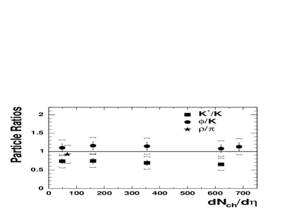
Figure 14: The $K^{*}/K^{-}$, $\phi/K^{-}$, and $\rho^{0}/\pi^{-}$ yield ratios as a function of $dN_{ch}/d\eta$ for Au+Au collisions at $\sqrt{s_{{}_{NN}}}\!=\!$ 200 GeV. All yield ratios have been normalized to the corresponding yield ratio measured in minimum bias $p+p$ collisions at the same c.m. system energy and indicated by the solid line. Both statistical and systematic uncertainties are shown.

The centrality dependence of the resonance yield ratios depicted in Fig. 14 suggests that the $\phi$ regeneration and the rescattering of the $\phi$ decay products are negligible, and the rescattering of the $K^{*0}$ decay products is dominant over the $K^{*0}$ regeneration and therefore the reaction channel $K^{*}\leftrightarrow K\pi$ is not in balance. As a result, the $K^{*0}/K^{-}$ yield ratio can be used to estimate the time between chemical and kinetic freeze-outs:

$$\frac{K^{*}}{K}|_{\text{kinetic}}=\frac{K^{*}}{K}|_{\text{chemical}}\times e^{-\Delta t/\tau},$$ (15)

where $\tau$ is the $K^{*}$ lifetime of 4 fm/$c$ and $\Delta t$ is the time between chemical and kinetic freeze-outs. If we use the minimum bias $p+p$ measurement of the $K^{*0}/K^{-}$ yield ratio as the one at chemical freeze-out and use the most central measurement of the $K^{*0}/K^{-}$ yield ratio in Au+Au collisions for the production at kinetic freeze-out, then under the assumptions that i) all the $K^{*}$s which decay before kinetic freeze-out are lost due to the rescattering effect and ii) there’s no regeneration effect, the time between chemical and kinetic freeze-outs is short and $\Delta t$ = 2 $\pm$ 1 fm/$c$. All the above assumptions reduce the estimated $\Delta t$. Thus the previous value is a lower limit of $\Delta t$ and it is not in conflict with the estimations ($>$6 fm/$c$) in meanpt . These two measurements together indicate that considerable resonance regeneration effect may happen even (about 4 fm/$c$) after chemical freeze-out.

V.5 Elliptic Anisotropy $v_{2}$

In non-central Au+Au collisions, the elliptic flow ($v_{2}$) is defined as the second harmonic coefficient of the Fourier expansion of the azimuthal particle distributions in momentum space art . The $K^{*0}$ $v_{2}$ can be calculated as:

$$v_{2}=\langle\text{cos}[2(\phi-\Psi_{r})]\rangle,$$ (16)

where $\phi$ is the $K^{*0}$ azimuthal angle in the momentum space, $\Psi_{r}$ denotes the actual reaction plane angle and $\langle\rangle$ indicates the average over all $K^{*0}$ in all events.

For each $K\pi$ pair, the reaction plane angle was estimated by the event plane ($\Psi_{2}$) which in turn was determined by using all the primary tracks except the kaon and pion tracks in the pair:

$$\Psi_{2}=\frac{1}{2}\times\tan^{-1}$$

$$\left(\frac{\sum_{i}\omega_{i}\sin(2\phi_{i})-\omega_{K}\sin(2\phi_{K})-\omega_{\pi}\sin(2\phi_{\pi})}{\sum_{i}\omega_{i}\cos(2\phi_{i})-\omega_{K}\cos(2\phi_{K})-\omega_{\pi}\cos(2\phi_{\pi})}\right),$$ (17)

where $\omega_{i}$ is the weight for each track used to optimize the event plane resolution, the subscripts $K$ and $\pi$ stand for the kaon and pion candidate track, respectively. This prevents the auto correlation between the $K\pi$ azimuthal angle $\phi_{K\pi}$ and the event plane angle $\Psi_{2}$ haibin .

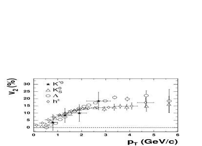
Figure 15: The $K^{*0}$ $v_{2}$ (filled stars) as a function of $p_{T}$ for minimum bias Au+Au collisions compared to the $K_{S}^{0}$ (open triangles), $\Lambda$ (open circles), and charged hadron (open diamonds) $v_{2}$. The errors shown are statistical only.

In minimum bias Au+Au collisions, the unlike-sign and mixed-event $K\pi$ pair invariant mass distributions are reconstructed in $\text{cos}[2(\phi-\Psi_{2})]$ bins and in $p_{T}$ bins. After the mixed-event background subtraction for each $\text{cos}[2(\phi-\Psi_{2})]$ bin and $p_{T}$ bin, the $K^{*0}$ yields are then obtained as a function of $\text{cos}[2(\phi-\Psi_{2})]$ for given $p_{T}$ bin. The average $\langle\text{cos}[2(\phi-\Psi_{2})]\rangle$ is then calculated for each $p_{T}$ bin. The finite resolution of the event plane angle, which is due to the limited number of tracks in the event plane calculation, reduces the measured $K^{*0}$ $v_{2}$. Thus the above obtained $\langle\text{cos}[2(\phi-\Psi_{2})]\rangle$ values are further corrected for an event plane resolution factor ($<1$) using the method presented in art . Figure 15 shows the $K^{*0}$ $v_{2}$ as a function of $p_{T}$ compared to the $K_{S}^{0}$, $\Lambda$, and charged hadron $v_{2}$ for minimum bias Au+Au collisions KsLav2 . A significant non-zero $K^{*0}$ $v_{2}$ is observed. Nevertheless, due to the large uncertainties on the $K^{*0}$ $v_{2}$ measurement, no significant difference is observed between the $K^{*0}$ $v_{2}$ and the $K_{S}^{0}$, $\Lambda$, and charged hadron $v_{2}$.

In order to calculate the contributions to the $K^{*}$ production from either direct quark or hadron combinations, the following function dong was used to fit the $K^{*0}$ $v_{2}$:

$$v_{2}(p_{T},n)=\frac{an}{1+\text{exp}[-(p_{T}/n-b)/c]}-dn,$$ (18)

where $a$, $b$, $c$ and $d$ are constants extracted by fitting to the $K_{S}^{0}$ and $\Lambda$ $v_{2}$ data points in dong , and $n$ is the open parameter standing for the number of constituent quarks. From the fit to the $K^{*0}$ $v_{2}$, $n=3\pm 2$ was obtained. Due to the large statistical uncertainties, it is difficult to identify the $K^{*}$ production fractions from direct quark combinations ($n=2$) or hadron combinations ($n=4$). About 15-20 times more Au+Au collision events were taken by the STAR experiment in the fourth RHIC run in 2004 which is expected to provide enough sensitivity for more precise calculations of $n$ to identify the $K^{*}$ from different production mechanism.

V.6 Nuclear Modification Factor

The number of binary collisions ($N_{bin}$) scaled centrality ratio ($R_{CP}$) is a measure of the particle production dependence on the size and density of the collision system and is closely related to the nuclear modification factor ($R_{AA}$). Recent measurements of the $\Lambda$ and $K_{S}^{0}$ $R_{CP}$ at RHIC KsLav2 have shown that in the intermediate $p_{T}$ region ($2<p_{T}<4$ GeV/$c$), the $\Lambda$ and $K_{S}^{0}$ $R_{CP}$ are significantly smaller than unity. These measurements suggest that high $p_{T}$ jets lose energy through gluon radiation while traversing through dense matter. It has also been observed that the $R_{CP}$ is significantly different for $\Lambda$ and $K_{S}^{0}$ with $p_{T}>2$ GeV/$c$. It is not clear whether this $R_{CP}$ difference is due to a mass or a particle species effect. The $K^{*}$ is a meson but has a mass that is close to the $\Lambda$ baryon mass. Thus, the measurement of the $K^{*}$ $R_{CP}$ may help in discriminating between mass or particle species effect at the intermediate $p_{T}$ region.

The $K^{*}$ $R_{CP}$ was obtained from the $p_{T}$ spectra of the top 10% and the 50-80% most peripheral Au+Au collisions. The $K^{*}$ $R_{AA}$ was calculated from the $p_{T}$ spectrum of the 10% most central Au+Au collisions and the $p_{T}$ spectrum of the minimum bias $p+p$ collisions.

The $K^{*}$ $R_{AA}$ and $R_{CP}$ as a function of $p_{T}$ compared to the $\Lambda$ and $K_{S}^{0}$ $R_{CP}$ are shown in Fig. 16. The $K^{*}$ $R_{AA}$ and $R_{CP}$ for $p_{T}<1.6$ GeV/$c$ are smaller than the $\Lambda$ and $K_{S}^{0}$ $R_{CP}$ indicating the strong rescattering of the $K^{*}$ daughters at low $p_{T}$. The rescattering of the $K^{*}$ decay products is weaker for $p_{T}>1.6$ GeV/$c$ since $K^{*}$ with larger $p_{T}$ are more likely to decay outside the fireball bleicher0 . Therefore, larger $p_{T}$ $K^{*}$ have a larger probability to be measured compared to low $p_{T}$ $K^{*}$. The $K^{*}$ $R_{AA}$ and $R_{CP}$ are closer to the $K_{S}^{0}$ $R_{CP}$ and different from the $\Lambda$ $R_{CP}$ for $p_{T}>1.6$ GeV/$c$. Thus, a strong mass dependence of the nuclear modification factor is not supported and a baryon-meson effect is favored in the particle production in the intermediate $p_{T}$ region.

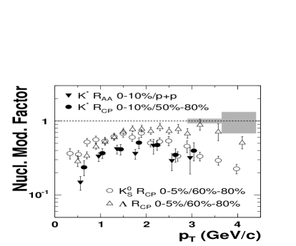
Figure 16: The $K^{*}$ $R_{AA}$ (filled triangles) and $R_{CP}$ (filled circles) as a function of $p_{T}$ compared to the $K_{S}^{0}$ (open circles) and $\Lambda$ (open triangles) $R_{CP}$. The errors shown are statistical only. The dashed line represents the number of binary collisions scaling. The widths of the grey bands represent the systematic uncertainties of $R_{AA}$ (left) and $R_{CP}$ (right) due to the model calculations of $N_{bin}$.

VI Conclusion

Results on the $K^{*0}$ and $K^{*\pm}$ resonance production in Au+Au and $p+p$ collisions measured with the STAR experiment at $\sqrt{s_{{}_{NN}}}$ = 200 GeV were presented. The $K^{*0}$ and $K^{*\pm}$ signals were reconstructed via their hadronic decay channels $K^{*0}\rightarrow K\pi$ and $K^{*\pm}\rightarrow K_{S}^{0}\pi^{\pm}$ at midrapidity.

The $K^{*0}/K$ yield ratios in Au+Au collisions were observed to be smaller than the ratio in $p+p$ interactions which may be interpreted in the context of finite cross sections in a late hadronic phase. The result suggests that the rescattering of the $K^{*0}$ decay products is dominant over the $K^{*0}$ regeneration and therefore the reaction channel $K^{*}\leftrightarrow K\pi$ is not in balance. As a result, the $K^{*0}/K^{-}$ yield ratio can be used to estimate the time between chemical and kinetic freeze-outs. Using the $K^{*0}/K^{-}$ yield ratio, the lower limit of the time between chemical and kinetic freeze-outs is estimated to be at least $2\pm 1$ fm/$c$.

A significant non-zero $K^{*0}$ elliptic flow $v_{2}$ was measured as a function of $p_{T}$ in minimum bias Au+Au collisions. Due to limited statistics, no conclusive statement can be made about the difference between the $K^{*0}$ $v_{2}$ and the $K_{S}^{0}$, $\Lambda$, and charged hadron $v_{2}$. The estimated number of constituent quarks for the $K^{*0}$ from the $v_{2}$ scaling according to Equation 18 is $3\pm 2$. Thus, larger statistics for Au+Au collision data are needed to identify the $K^{*}$ production fractions from direct quark combinations or hadron combinations.

The $K^{*0}$ nuclear modification factors $R_{AA}$ and $R_{CP}$ were measured as a function of $p_{T}$. Both the $K^{*0}$ $R_{AA}$ and $R_{CP}$ are found to be closer to the $K_{S}^{0}$ $R_{CP}$ and different from the $\Lambda$ $R_{CP}$ for $p_{T}>2$ GeV/$c$. A strong mass dependence of the nuclear modification factor is not observed. This establishes a baryon-meson effect over a mass effect in the particle production at the intermediate $p_{T}$ region.

VII Acknowledgement

We thank the RHIC Operations Group and RCF at BNL, and the NERSC Center at LBNL for their support. This work was supported in part by the HENP Divisions of the Office of Science of the U.S. DOE; the U.S. NSF; the BMBF of Germany; IN2P3, RA, RPL, and EMN of France; EPSRC of the United Kingdom; FAPESP of Brazil; the Russian Ministry of Science and Technology; the Ministry of Education and the NNSFC of China; Grant Agency of the Czech Republic, FOM and UU of the Netherlands, DAE, DST, and CSIR of the Government of India; Swiss NSF; and the Polish State Committee for Scientific Research.

References

(1) T. Blum et al., Phys. Rev. D 51, 5153 (1995).
(2) R. Rapp, Phys. Rev. C 66, 017901 (2002).
(3) R. Rapp and E.V. Shuryak, Phys. Rev. Lett. 86, 2980 (2001).
(4) C. Song and V. Koch, Phys. Rev. C 55, 3026 (1997).
(5) J. Rafelski et al., Phys. Rev. C 64, 054907 (2001).
(6) G. Brown and M. Rho, Phys. Rev. Lett. 66, 2720 (1991).
(7) R. Rapp, Nucl.Phys. A 725, 254 (2003).
(8) E.V. Shuryak and G. Brown, Nucl. Phys. A 717, 322 (2003).
(9) J. Schaffner-Bielich, Phys. Rev. Lett. 84, 3261 (2000).
(10) R. Rapp and J. Wambach, Adv. Nucl. Phys. 25, 1 (2000).
(11) J.M. Link et al., Phys. Lett. B 535,
43 (2002).
(12) J. Adams et al., Phys. Rev. Lett. 92, 092301 (2004).
(13) M. Bleicher and H. Stöcker, J. Phys. G
30, S111 (2004).
(14) R.S. Longacre, nucl-th/0303068.
(15) P. Braun-Munzinger (private communication).
(16) P.F. Kolb and M. Prakash, Phys. Rev. C 67, 044902 (2003).
(17) W. Broniowski et al., Phys. Rev. C 68, 034911 (2003).
(18) H.W. Barz et al., Phys. Lett. B 265,
219 (1991).
(19) S. Pratt and W. Bauer, Phys. Rev. C 68, 064905
(2003).
(20) P. Granet et al., Nucl. Phys. B 140,
389 (1978).
(21) M. Bleicher et al., Phys. Lett. B 530, 81 (2002).
(22) S.D. Protopopescu et al., Phys. Rev. D 7, 1279 (1973).
(23) M.J. Matison et al., Phys. Rev. D 9, 1872 (1974).
(24) M. Bleicher et al., J. Phys. G 25, 1859 (1999).
(25) Z.-W. Lin and C.M. Ko, Phys. Rev. Lett. 89, 202302 (2002).
(26) S. S. Adler et al., Phys. Rev. C 69, 034909 (2004).
(27) J. Adams et al., Phys. Rev. Lett. 92 052302 (2004).
(28) C. Nonaka et al., Phys. Rev. C 69, 031902 (2004).
(29) C. Adler et al., Phys. Rev. Lett. 89,
202301 (2002).
(30) M. Anderson et al., Nucl. Instrum. Meth. A 499, 659 (2003).
(31) C. Adler et al., Phys. Rev. Lett. 87,
112303 (2001).
(32) K. Hagiwara et al., Phys. Rev. D 66, 010001 (2002).
(33) C. Adler et al., Phys. Lett. B 595, 143 (2004).
(34) C. Adler et al., Phys. Rev. Lett. 89, 092301 (2002).
(35) C. Adler et al., Phys. Rev. C 66, 061901(R) (2002).
(36) C. Adler et al., Phys. Rev. C 65, 041901(R) (2002).
(37) J. Adams et al., to be published in Phys. Lett. B, nucl-ex/0406003.
(38) K. Adcox et al., Phys. Rev. Lett. 89, 092302 (2002).
(39) H. Zhang, Ph.D. thesis, Yale University (2004).
(40) L. Gaudichet, Ph.D. thesis, SUBATECH, France (2003).
(41) C. Adler et al., Phys. Rev. Lett. 89, 272302 (2002).
(42) J. Adams et al., Phys. Rev. Lett. 92, 112301
(2004).
(43) F. Becattini, Nucl. Phys. A 702, 336 (2002).
(44) C. Adler et al., Phys. Rev.
Lett. 87, 112303 (2001).
(45) T. Sjostrand et al., Computer Physics
Commun. 135, 238 (2001).
(46) G Wilk and Z. Wlodarczyk, Phys. Rev. Lett. 84, 2270 (2000).
(47) E. Schnedermann, J. Sollfrank, and U. Heinz,
Phys. Rev. C 48, 2462 (1993).
(48) H. Albrecht et al., Z. Phys. C 61, 1 (1994).
(49) M. Derrick et al., Phys. Lett. B 158, 519 (1985).
(50) K. Abe et al., Phys. Rev. D 59, 052001 (1999).
(51) Y. Pei, Z. Phys. C 72, 39 (1996).
(52) J. Canter et al., Phys. Rev. D 20, 1029 (1979).
(53) M. Aguilar-Benitez et al., Z. Phys. C 50, 405 (1991).
(54) D. Drijard et al., Z. Phys. C 9, 293 (1981).
(55) T. Akesson et al., Nucl. Phys. B 203, 27 (1982).
(56) P. Braun-Munzinger et al., Phys. Lett. B 518, 41 (2001);
J. Stachel (private communication).
(57) A. Poskanzer and S. Voloshin, Phys. Rev. C 58, 1671 (1998).
(58) X. Dong et al., Phys. Lett. B 597, 328 (2004).