Particle and light fragment emission in peripheral heavy ion collisions at Fermi energies

Abstract

A systematic investigation of the average multiplicities of light charged particles and intermediate mass fragments emitted in peripheral and semiperipheral collisions is presented as a function of the beam energy, violence of the collision and mass of the system. The data have been collected with the Fiasco setup in the reactions ⁹³Nb+⁹³Nb at 17, 23, 30, 38 A MeV and ¹¹⁶Sn+¹¹⁶Sn at 30, 38 A MeV. The midvelocity emission has been separated from the emission of the projectile-like fragment. This last component appears to be compatible with an evaporation from an equilibrated source at normal density, as described by the statistical code Gemini at the appropriate excitation energy. On the contrary, the midvelocity emission presents remarkable differences for what concerns both the dependence of the multiplicities on the energy deposited in the midvelocity region and the isotopic composition of the emitted light charged particles.

I Introduction

In recent years many works (see, e.g., Łukasik et al. (1997); Plagnol et al. (1999); Piantelli et al. (2002); Milazzo et al. (2002); Mangiarotti et al. (2004) and references therein) were devoted to the investigation of Light Charge Particle (LCP) and Intermediate Mass Fragment (IMF) emission in semiperipheral and peripheral heavy ion collisions at Fermi energies. It is well established that these reactions show mainly a binary character, with two heavy remnants in the exit channel, possibly undergoing a subsequent sequential fission Stefanini et al. (1995). Among the various features of the emission, one in particular raised a lot of interest: a large amount of emission is located at midvelocity (i.e., close to the center-of-mass velocity), mainly for the IMFs but also for lighter particles Plagnol et al. (1999); Łukasik et al. (1997); Bowman et al. (1993); Montoya et al. (1994); Tõke et al. (1996); Dempsey et al. (1996); Piantelli et al. (2002). The origin of this phenomenon is still actively debated. Possible interpretations range from, e.g., a kind of neck rupture Łukasik et al. (1997); Baran et al. (2004), due to mechanical and/or chemical instabilities, to a fast statistical emission from one of the heavy fragments perturbed by the proximity of the other heavy remnant Botvina et al. (1999); Botvina and Mishustin (2001).

In a previous work Piantelli et al. (2002), by means of a three-body Coulomb trajectory calculations, we put into evidence two components in the experimental IMF emission pattern: a fast emission from the phase space region in between the two heavy remnants, somewhat reminiscent of a neck fragmentation or a participant-spectator model, and a later emission from the (possibly deformed) surface of the heavy fragments. The latter mechanism may be interpreted as the evolution of the fast oriented fission mechanism Stefanini et al. (1995); Casini et al. (1993); Bocage et al. (2000) toward very large mass asymmetries. Similar conclusions were drawn in a more recent paper De Filippo et al. (2005), using the same basic approach of Coulomb trajectory calculations.

The midvelocity emission is particularly evident in very peripheral reactions (b/b${}_{\mathrm{graz}}\geq$ 0.9), where the kinematics of the collision is relatively simple and the multiplicity of LCPs (and IMFs) emitted from the two fully accelerated main fragments is quite small (about 0.3 LCP per event in Ref. Piantelli et al. (2002)). As a consequence, the investigation of peripheral collisions is a fundamental tool in order to shed more light on the production mechanism and on its evolution with the beam energy. The short interaction times typical of these collisions can also be used to investigate isospin diffusion and equilibration in collisions between nuclei with different N/Z ratio (see Di Toro et al. (2006) and references therein).

In Mangiarotti et al. (2004) we found that in peripheral collisions the energy stored inside the midvelocity matter and the excitation energy of the quasi-projectile have similar values. This evidence suggested a larger energy density ($>$ 7 MeV/nucleon) in the midvelocity “source”, with respect to the excited quasi-projectile ($\leq$ 2 MeV/nucleon), since the mass localized at midvelocity is certainly smaller (the value would even rise to $\approx$13 MeV/nucleon if the mass of the midvelocity “source” were identified with the total mass of its emitted particles). Similar conclusions were drawn from the comparison of transverse velocities too Hudan et al. (2005). If one assumes, as stated for example in Durand (1998), that in central collision the multifragmentation process starts at excitation energies of the source greater than $\approx$3 A MeV, then the midvelocity emissions might be interpreted as a first appearance of the multifragmentation process Baran et al. (2004). Indeed it was also claimed that midvelocity fragments associated with midperipheral and central collisions present similar characteristics Hudan et al. (2005).

This paper presents a systematic investigation of the average multiplicities of LCPs and IMFs emitted in peripheral and semiperipheral collisions of symmetric systems at Fermi energies. The evolution of the multiplicities is studied as a function of the excitation energy of the emitting “source”, mass of the system and beam energy. Section II briefly describes the experimental setup Fiasco Bini et al. (2003) and the investigated reactions. Section III discusses the event selection and describes the analysis methods for separating the evaporative and midvelocity components of the emissions. Section IV presents the obtained results on the particle multiplicities and their scaling with the excitation energy and mass of the “source” and the beam energy, while conclusions are drawn in Section V. Some more technical points are presented in the Appendices.

II Experimental setup

The results presented in this paper were obtained in a systematic study Piantelli (2001); Piantelli et al. (2002); Mangiarotti (2003); Mangiarotti et al. (2004) of heavy ion collisions performed at the Superconducting Cyclotron of the Laboratori Nazionali del Sud of INFN in Catania.

Beams of ⁹³Nb at 17.0, 23.0, 29.5 and 38.1 A MeV  and of ¹¹⁶Sn at 29.6 and 38.1 A MeV were used to bombard ⁹³Nb and ¹¹⁶Sn targets of about 200 $\mu$g/cm² thickness. This paper concerns solely the symmetric collisions ⁹³Nb + ⁹³Nb and ¹¹⁶Sn + ¹¹⁶Sn, for which some parameters, calculated using the Bass interaction distance R_int Bass (1980), are listed in Table 1.

The experimental data have been measured with the Fiasco setup (described with more details in Bini et al. (2003); Piantelli (2001)), a multidetector particularly well suited for the study of peripheral and semiperipheral reactions, where only few heavy remnants are produced. In fact, as a characteristic feature, this setup includes 24 large-area position-sensitive Parallel Plate Avalanche Detectors (PPAD) Charity et al. (1991); Stefanini et al. (1995) covering about 70% of the forward hemisphere. They are fully efficient for heavy fragments with Z$\gtrsim$10 and are used to measure velocity vectors with very low detection thresholds ($\sim$ 0.1 A MeV) and good accuracy (position and time-of-flight resolutions of 2-4 mm and 700 ps (FWHM), respectively, with flight-paths of about 3.5 m for $\theta\lesssim 10^{\circ}$). In this way it is possible to simultaneously detect both the projectile-like fragment (PLF) and the very slow target-like fragment (TLF) even in the most peripheral collisions and to perform a kinematic reconstruction of the events Casini et al. (1989).

Behind the most forward PPADs, a mosaic of 96 Silicon telescopes allows to measure the energy, the charge, and the final mass (by means of the time-of-flight) of the PLF. Each telescope (with 28$\times$28 cm² active area) consists of a 200$\mu$m $\Delta$E detector followed by a 500$\mu$m E_res detector.

Finally, the setup is completed by 182 three-layer phoswich scintillation telescopes, mounted behind most of the PPADs and covering about $30\%$ of the forward hemisphere (plus a reduced sampling in the backward hemisphere), which are devoted to the detection of light charged particles and intermediate mass fragments. The phoswiches allow isotopic identification of Hydrogen (and in some cases of Helium) isotopes and charge identification of heavier products up to $Z\sim$15–20 (with a threshold of about 3-3.5 A MeV) and give a direct measurement of the time of flight (and hence of the velocity) of all these reaction products, without any need for tricky and time-consuming energy calibrations of the scintillators.

The experiment was performed together with the hodoscope Hodo-Ct Immè et al. (March 1993) of the Temperature experiment Sfienti et al. (2004), but its data have not been used here.

The results presented in this paper are focused on binary events – by far prevailing in peripheral and semiperipheral collisions – with only two large reaction remnants (Z$\gtrsim$10) detected by the gas counters, and on the associated multiplicities of LCPs and light IMFs with Z=3–7.

Table 1: Some calculated reaction parameters

	93Nb+93Nb				116Sn+116Sn
E/A (MeV)	17	23	30	38	30	38
E${}_{\mathrm{\,in}}^{\mathrm{\;c.m.}}$ (MeV)	791	1069	1374	1772	1715	2210
$v_{\mathrm{rel}}$ (mm/ns)	57.3	66.6	75.6	85.8	75.6	85.8
$\theta_{\mathrm{graz}}^{\mathrm{Lab}}$ (deg)	7.8	5.5	4.2	3.2	4.8	3.6
$b_{\mathrm{graz}}$ (fm)	11.2	11.6	11.9	12.1	12.5	12.8
$\ell_{\mathrm{graz}}$ ($\hbar$)	470	568	660	762	865	1002
$\sigma_{\mathrm{reac}}^{\mathrm{\,calc}}$ (mb)	3938	4260	4462	4621	4942	5143

III Experimental data

III.1 The choice of an “ordering parameter”

For a meaningful sorting of the data in homogeneous bins of increasing centrality, one needs an experimental variable which is expected to have a monotonic and possibly narrow relationship with the impact parameter of the collision. This “sorting” variable should also be -as much as possible- independent of the studied observables, in order to avoid (or reduce) autocorrelation effects.

Global variables (like multiplicities, flow angles, transverse energies, etc.) are not used in the present work, as they are best suited for experiments covering very large solid angles (close to 4$\pi$). Therefore other variables, related to more particular aspects of the reaction, must be considered. Since the main subject of this paper is the emission of LCPs and IMFs in binary collisions, it is natural to restrict the choice to variables which make use of experimental information concerning the two main reaction partners (like, e.g., the secondary charge $Z_{\mathrm{sec}}$ of the PLF residue, or its secondary velocity $v_{\,\mathrm{PLF}}$, or the relative velocity $v_{\mathrm{rel}}$ between PLF and TLF).

Our choice is a variable Schröder and Huizenga (1977) defined as

$$\mathrm{TKEL}=\mathrm{E}_{\mathrm{\,in}}^{\mathrm{\;c.m.}}\,-\,\tfrac{1}{2}\,\tilde{\mu}\,{v_{\mathrm{rel}}^{\,2}},$$ (1)

where E${}_{\mathrm{\,in}}^{\mathrm{\;c.m.}}$ is the center-of-mass (c.m.) energy of the collision in the entrance channel, $v_{\mathrm{rel}}$ the reconstructed relative velocity and $\tilde{\mu}$ the reduced mass calculated with the masses obtained from the kinematic analysis.

It is to be noted that -by definition- the kinematic method constrains the primary masses of the two reaction partners to add up to the total mass of the system. Thus, while at low incident energies, where reactions are strictly binary, TKEL may truly represent the “Total Kinetic Energy Loss” of the collision – namely the total amount of kinetic energy transferred from the relative motion into internal energy of the colliding system – it is important to note that at Fermi energies, where the presence of a sizable midvelocity emission causes an overestimation of the kinematically determined $\tilde{\mu}$, this interpretation is no longer correct. Therefore, in this work TKEL is used just as an ordering parameter for sorting the events in bins of increasing centrality.

Table 2: Reaction cross sections

	93Nb + 93Nb				116Sn+116Sn
E/A (MeV)	17	23	30	38	30	38
$\sigma_{2b}^{\mathrm{\,exp}}$ (mb)	3210	2840	2750	2810	2670	3010
$\sigma_{3b}^{\mathrm{\,exp}}$ (mb)	640	940	940	790	1030	980
$\sigma_{\mathrm{2b}}^{\mathrm{\,exp}}/\sigma_{\mathrm{reac}}^{\mathrm{\,calc}}$	82%	67%	62%	61%	54%	58%
$\sigma_{\mathrm{2b+3b}}^{\mathrm{\,exp}}/\sigma_{\mathrm{reac}}^{\mathrm{\,calc}}$	98%	89%	83%	78%	75%	77%

A short discussion about the relationship of TKEL with other possible sorting variables is also presented in Appendix A, together with an estimation of the correspondence between TKEL and impact parameter obtained both by means of model calculations and experimentally via a direct integration of the reaction cross section. We anticipate here that, for a given colliding system, equal values of TKEL correspond to similar impact parameters regardless of the bombarding energy, at least as far as (semi-)peripheral collisions are concerned. When the system is changed (in our case from Nb+Nb to Sn+Sn), a given value of TKEL indicates a somewhat larger impact parameter for the heavier system, as expected from the larger nuclear radii.

III.2 The cross sections

For each reaction, the simultaneous measurement (via a dedicated and suitably down-scaled “singles” trigger) of elastically scattered projectiles hitting the most forward gas detectors has been used for determining the conversion factor (“millibarn-per-count”). After correcting for the experimental filter, this allows to perform a quantitative estimate of the experimental cross sections pertaining to the detected two- and three-body events. They are summarized, for all investigated reactions, in the first and second row of Table 2, while the third row indicates the percentage of the calculated total reaction cross section which is accounted for by these two channels (more details are given in Appendix A).

The third row shows that the exit channel with two heavy remnants remains the dominant one even at the highest investigated energies, where it still accounts for more than half of $\sigma_{\mathrm{reac}}^{\mathrm{\,calc}}$, thus demonstrating the persistence of the binary or quasi-binary character of the reactions. The three-body channel, which is likely to be due to sequential fission or to the “fast oriented fission” Casini et al. (1993); Stefanini et al. (1995) of one of the two main fragments, adds an appreciable contribution. For the ⁹³Nb beams (where more beam energies have been studied) it is interesting to note that at 17 A MeV the two- and three-body channels account for nearly 100% (within errors) of the whole reaction cross section and that this percentage decreases with increasing bombarding energy. This behavior may be due to the progressive opening of new reaction channels (four- or more-body reactions, possibly multifragmentation). However, even at the highest energy of 38 A MeV, the two- and three-body exit channels altogether still represent about 75% of $\sigma_{\mathrm{reac}}^{\mathrm{\,calc}}$.

The main uncertainty on the quoted numbers concerns the cross sections for two-body events. It mainly arises from the difficulty of separating elastic and quasi-elastic scattering in the vicinity of the grazing angle. The experimental data have been integrated starting from the calculated grazing angles of Table 1, after having verified that they agree with the experimental “quarter-point” angles within a few tenths of degree. Such an uncertainty in angle corresponds to an uncertainty of the order of 200-300 mb on the cross sections and of about 5–6% on the percentages in the last row.

III.3 The emission pattern

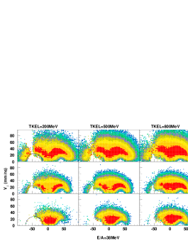
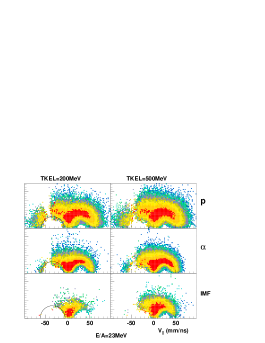
Figure 1: (color) Experimental yields (corrected for the setup efficiency) of protons (upper row), $\alpha$ particles (middle row) and IMFs with $Z$=3–7 (lower row) for ⁹³Nb + ⁹³Nb at 38 (left panels) and 23 A MeV (right panels). Yields – with logarithmic level spacing in factor-of-2 steps – are in the plane ($v_{\,\parallel},v_{\,\perp}$), with respect to the PLF-TLF separation axis, the origin being in the center-of-mass system. Columns refer to 100-MeV wide TKEL bins centered, from left to right, at 200, 500, 800 MeV (at 38 A MeV) and 200, 500 MeV (23 A MeV). The circles in the TKEL=200 MeV panels show regions affected by velocity thresholds (due to the thin fast-plastic scintillators of the phoswich telescopes, see Bini et al. (2003)).

The shape of the emission pattern of LCPs and IMFs can be best appreciated from the distribution of the experimental yields in the ($v_{\,\parallel}$,$v_{\,\perp}$) plane, where $v_{\,\parallel}$ and $v_{\,\perp}$ are the velocity components (in the c.m. reference system) parallel and perpendicular, respectively, to the asymptotic PLF-TLF separation axis (for the TKEL range addressed in this work, the separation axis remains in most cases within about 10^∘ from the beam axis). As the solid angle coverage of the Fiasco setup, although large, is however significantly smaller than 4$\pi$, it is first necessary to correct the data for the limited geometrical coverage of the setup and for the low-energy identification thresholds Piantelli (2001).

The correction Piantelli (2001); Mangiarotti (2003) is obtained from a Monte Carlo simulation which produces - for each particle species - a random isotropic emission. In fact, it has been verified that, thanks to the large acceptance and axial symmetry of the setup, the obtained correction is largely independent of the specific emission pattern used in the simulation. Therefore the emission adopted in the simulation homogeneously fills a sphere in phase space, centered in the c.m. origin with radius $v_{\mathrm{max}}$= 120 mm/ns, thus covering all regions which are relevant for the processes under study. The velocity vector of each LCP or IMF is then transformed into the laboratory reference frame and the appropriate experimental filter of the Fiasco setup is applied (geometry and identification thresholds of the phoswich detectors). In order to mimic as closely as possible the binary reaction step, all its relevant parameters (like the orientation of the PLF-TLF separation axis and the PLF and TLF c.m. velocities) are those obtained with the kinematic reconstruction directly from the measured two-body events. Using these parameters, the procedure allows to determine, for each cell in the ($v_{\,\parallel}$, $v_{\,\perp}$, $\phi$) space and for successive bins in TKEL, an average correction factor, which is obtained as the ratio between the number of generated particles and the number of particles surviving the experimental filter of the setup. (Here $\phi$ is the out-of-plane angle with respect to the reaction plane; this coordinate was explicitly considered for a better efficiency correction in case of possible out-of-plane anisotropies in the experimental data, e.g., due to angular momentum effects). When analyzing the actual data, the experimental yields of each particle species are multiplied, cell-by-cell, by the now described correction factors.

As an example of the obtained distributions, Fig. 1 shows the efficiency-corrected experimental yields of protons, $\alpha$ particles and IMFs with $Z$=3–7 (first, second and third row, respectively) in the reaction ⁹³Nb + ⁹³Nb at 38 and 23 A MeV for three and two bins of TKEL, respectively. In this presentation, in absence of instrumental effects, the average positions of the PLF and TLF emitters lie -by definition- on the horizontal axis, symmetrically with respect to the c.m. origin. One clearly sees characteristic circles around the positions of PLF and TLF, indicating a Coulomb-dominated emission from these sources, as it is expected for the sequential decay of such highly excited systems. (In the case of TLF, the inner part of the Coulomb circles is marginally affected by the velocity thresholds.) It has also to be noted that, since yields are presented in Fig. 1 – and not invariant cross sections – the intensity of an isotropic emission must gradually decrease along the Coulomb circles while approaching the $v_{\,\parallel}$-axis, until it vanishes when it reaches this axis. At parallel velocities intermediate between those of PLF and TLF, one observes an additional contribution, the so-called “midvelocity” (or “neck”) emission. Although present for all particle species, this emission is particularly evident and important for $\alpha$ particles and even more for IMFs.

The Fiasco setup has a much better solid angle coverage in forward direction, where -in addition- thresholds effects do not play any practical role, because the energies of all particles in the lab-system are greater than $\approx$ 4 A MeV already for the collision at 17 A MeV. On the contrary, the solid angle coverage in backward direction is limited. It has to be noted that phase space cells with small average efficiency have large correction factors, which amplify the statistical fluctuations of the experimental data, and cells with zero efficiency cannot be corrected at all. This is the reason why in the backward hemisphere of the laboratory reference frame (corresponding in c.m. to $v_{\,\parallel}\lesssim-\,43$ mm/ns for the reaction at 38 A MeV and to $v_{\,\parallel}\lesssim-\,33$ mm/ns for that at 23 A MeV) the applied corrections are not as effective as in the forward hemisphere.

Finally, as the results presented in this paper concern LCPs and IMFs emitted in peripheral binary reactions, the data need to be corrected for the presence of a background of events with a higher multiplicity of heavy fragments, of which only two have been detected. This background of incomplete events (a few percent) has been estimated using the measured three-body events (with the procedure described in Ref. Casini et al. (1989)) and subtracted from all the data presented in this paper.

III.4 The particle multiplicities

The average multiplicities of charged particles were obtained from the (efficiency corrected and background subtracted) experimental distributions of p, d, t, $\alpha$ and IMFs, some examples of which are shown in Fig. 1.

An advantage of using symmetric collisions is that the forward-going particles (those with $v_{\,\parallel}\geq 0$ in c.m.) must have the same average characteristics as the backward-going ones. Therefore, because of the already mentioned much better quality of the data, all presented multiplicities refer only to particles emitted in the forward hemisphere of the c.m. reference frame (of course, the average multiplicities for the whole colliding system can be obtained by simply doubling the presented values).

Figure 2: Average total charge Z_tot of forward-going products (full dots) and average secondary charge Z_sec of PLF (open dots) in ⁹³Nb + ⁹³Nb and ¹¹⁶Sn + ¹¹⁶Sn at 30 A MeV. Dashed lines indicate the value of the projectile charge.

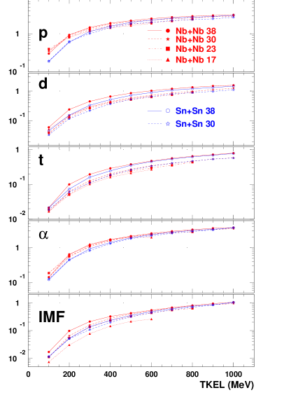
Figure 3: (color online) Experimental efficiency-corrected average multiplicities of (forward-emitted) p, d, t, $\alpha$ and IMFs ($Z$=3–7) as a function of TKEL, for ⁹³Nb+⁹³Nb (full symbols) and ¹¹⁶Sn+¹¹⁶Sn (open symbols). The bombarding energies are 17 (triangles, dotted lines), 23 (squares, dot-dashed lines), 30 (stars, dashed lines) and 38 A MeV (circles, full lines); the lines are to guide the eye.

The symmetry of the system also allows to check the quality of the applied efficiency corrections. In fact, whatever the reaction mechanism, by adding up the charges of forward emitted LCPs and IMFs to the charge of the PLF residue, one should reproduce -on average- just the projectile charge (of course, this can be done only for that subset of the events in which the PLF residue was detected and identified in one of the Silicon telescopes). As an example of the quality of this check, the full dots of Fig. 2 show the average total forward-emitted charge for the ⁹³Nb + ⁹³Nb and ¹¹⁶Sn + ¹¹⁶Sn collisions at 30 A MeV: within about half a charge unit, the value of the projectile (dotted line) is well reproduced, thus giving confidence in the present analysis. The rapidly widening gap between the full dots and the open ones (which represent the average secondary charge Z_sec of the detected PLF) gives a visual indication of the rising amount of charges removed by the LCP and IMF emissions with increasing TKEL.

The obtained average multiplicities (of forward-going particles) are shown in Fig. 3 for the systems ⁹³Nb + ⁹³Nb (full symbols) and ¹¹⁶Sn + ¹¹⁶Sn (open symbols) at the bombarding energies of 17, 23, 30 and 38 A MeV (triangles, squares, stars and circles, respectively). The statistical errors are smaller than the symbols and the lines are just to guide the eye.

Although data corresponding to more violent collisions have been acquired too, the present analysis is limited to peripheral and semiperipheral collisions through a restriction of the TKEL range (from $\leq$600 MeV for the reaction at 17 A MeV up to $\leq$1000 MeV for those at 38 A MeV). This has the twofold advantage of allowing a clear and unambiguous distinction between PLF and TLF (in c.m. the forward-flying heavy remnant is always the PLF) and of limiting the study to regions where the binary exit channel is the dominant one. In the considered TKEL ranges the binary exit channel remains approximately symmetric in mass, as indicated by comparable values of the c.m. velocities of the two main fragments. Only in the last considered TKEL bins weak tails of more asymmetric mass splittings appear. In the analysis, the requirement 0.4 $\leq v^{\mathrm{c.m.}}_{\mathrm{PLF}}/(v^{\mathrm{c.m.}}_{\mathrm{PLF}}+v^{\mathrm{c.m.}}_{\mathrm{TLF}})\leq\;$0.6 has been used to reject these tails, which are strongly contaminated by incompletely detected three-body events.

Qualitatively, all multiplicities display a similar behavior, with a strong dependence on TKEL and a much weaker one on bombarding energy and mass of the system. Starting from small TKEL they all increase rapidly but then tend to flatten at large TKEL values. Over the range of TKEL considered here, the multiplicities span about one order of magnitude -or slightly more- for the most abundant species (protons and $\alpha$ particles, with multiplicities up to several particles per event) and about two orders of magnitude for the rarer reaction products (which barely reach multiplicities of one per event at the highest values of TKEL).

III.5 Evaporative and midvelocity emissions

In order to disentangle the midvelocity emission from the sequential evaporation of the PLF, it is convenient to make a coordinate transformation into the reference frame of the PLF, namely a frame with the $v_{\,\parallel}$-axis still oriented along the asymptotic PLF-TLF separation axis, but with the origin on the PLF itself. A relativistic Lorentz transformation has been applied (instead of simpler Galilean one), in order to avoid distortions of the angular distribution of the fastest particles; this comes out to be necessary in particular for protons, which may have lab-velocities as large as 30% of the speed of light. An example of the obtained yield in the ($v_{\,\parallel}^{\,\mathrm{PLF}},v_{\,\perp}^{\,\mathrm{PLF}}$) plane is shown in Fig. 4(a) for protons, at TKEL= 800 MeV, in the reaction ⁹³Nb + ⁹³Nb at 38 A MeV. The corresponding angular distribution, presented in Fig. 4(b), is obtained by plotting the proton yield as a function of $\cos(\theta_{\mathrm{PLF}})$, where $\theta_{\mathrm{PLF}}$ is the polar emission angle between the velocity of the protons in the PLF frame and the PLF-TLF separation axis, as sketched in Fig. 4(e): thus $\cos\,(\theta_{\mathrm{PLF}})=1$ corresponds to a forward emission along the flight direction of the PLF in the c.m. system.

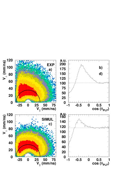
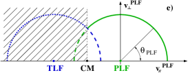
Figure 4: (color) Experimental (a) and simulated (c) yields of protons in the ($v_{\,\parallel}^{\,\mathrm{PLF}},v_{\,\perp}^{\,\mathrm{PLF}}$) plane (with origin in the PLF reference frame) and corresponding experimental (b) and simulated (d) distributions of $d\sigma/d\cos(\theta_{\mathrm{PLF}})$ for TKEL=800 MeV in the reaction ⁹³Nb+⁹³Nb at 38 A MeV. Only forward-going particles (i.e., with $v_{\,\parallel}$ in the lab-system larger than the c.m. velocity) are considered –as sketched in (e)– and this causes the yields to vanish for $v_{\,\parallel}\lesssim$ -35 mm/ns in panels (a) and (c).

For comparison, Fig. 4(c) and (d) show the corresponding results obtained with a Monte Carlo simulation, where only an isotropic evaporation from the fully accelerated PLF and TLF is considered, as sketched by the two circles in Fig. 4(e). At small TKEL the emissions from PLF and TLF are well separated from each other and the $\cos\,(\theta_{\mathrm{PLF}})$-distribution is flat. At larger TKEL, on the contrary, the distribution presents a dip at $\cos\,(\theta_{\mathrm{PLF}})$= -1 and a bump at less negative values of $\cos\,(\theta_{\mathrm{PLF}})$, as shown in Fig. 4(d). This distortion of the backward part of the angular distribution is due to the merging of the two evaporative emissions (from PLF and TLF) when the relative velocity of the two sources is reduced: as shown in Fig. 4(e), selecting the forward-going particles (in c.m.) one misses the dash-dotted part of the PLF circle, but includes the dashed part of the TLF circle. Nonetheless, thanks to the symmetry of the system, the yields and the multiplicities are correctly evaluated. In fact, with respect to the flat behavior of the forward part of the $\cos\,(\theta_{\mathrm{PLF}})$-distribution [dashed line in Fig. 4(d)], the excess area in the bump neatly compensates the deficit around -1.

When comparing the experimental angular distribution of Fig. 4(b) with the simulated one of Fig. 4(d), it becomes evident that: (i) The shapes are qualitatively similar. (ii) The forward part of the experimental angular distribution, in the vicinity of $\cos\,(\theta_{\mathrm{PLF}})$ = 1 is indeed flat, as expected for an evaporative (nearly isotropic) component. (iii) The broad bump around $\cos(\theta_{\mathrm{PLF}})$ = - 0.5 overcompensates the dip near -1, thus confirming the presence of an additional backward emission (with respect to the PLF frame), namely an emission in the midvelocity region of the phase-space. (iv) The tail of the bump extends well into the forward hemisphere in the PLF frame Mangiarotti et al. (2004).

Thus, as already noted in Mangiarotti et al. (2004), the analysis of the experimental angular distribution suggests the superposition of two emission components, namely one from the PLF and one from “midvelocity”. As it will be shown in Sec. IV.2, there are good arguments for interpreting the first component as an evaporation from the excited PLF; therefore the two terms, evaporation and PLF-emission, will be used interchangeably in the rest of this paper. On the basis of the previous point (ii), a decomposition can be attempted, provided that the shape of the whole evaporative component can be reliably estimated. Since evaporation must be forward-backward symmetric in the frame of the emitter, it is usual (see, e.g., Plagnol et al. (1999); D’Agostino et al. (1999)) to estimate the total evaporation from the PLF by simply doubling its forward emission. This may work at higher bombarding energies (where evaporation from PLF/TLF and midvelocity emissions are well separated in phase space), but the above point (iv) shows that, even at the highest energy of 38 A MeV, the usual procedure would result in a significant contamination from the midvelocity emission. Which part of the angular distribution can be considered sufficiently clean depends on the bombarding energy, on the chosen TKEL bin and also on the considered particle species. However, for the reactions of this paper, the range $0^{\circ}\leq\theta_{\mathrm{PLF}}\leq 45^{\circ}$ (i.e., $0.7\leq\cos(\theta_{\mathrm{PLF}})\leq 1$) is a reasonable compromise which can be used in almost all cases. (We verified that the total evaporative multiplicities remain stable within $\pm$10% if the data are taken, e.g., in the narrower range $0^{\circ}\leq\theta_{\mathrm{PLF}}\leq 30^{\circ}$ while progressively larger deviations appear if data beyond $45^{\circ}$ are included, see Appendix B.).

In order to estimate, from the data measured at forward angles, the total yield of the PLF component, it is necessary to make some hypothesis on the angular distribution $d\sigma/d\cos(\theta_{\mathrm{PLF}})$, which depends on the spin of the emitter. In fact this distribution is flat only in case of an isotropic evaporation from a zero-spin source, while in case of non-zero spin the evaporation tends to concentrate in a plane perpendicular to the spin direction, giving origin to an U-shaped $\cos(\theta_{\mathrm{PLF}})$ distribution: the larger the spin (or the heavier the evaporated particle), the stronger the effect. According to a detailed study of the correlations of the emitted particles with both the PLF and TLF Mangiarotti (2003); Mangiarotti et al. , it was estimated that in the reaction ⁹³Nb + ⁹³Nb at 38 A MeV the spin of the PLF is negligible at low TKEL, but rises to $15\pm 5\hbar$ and $30\pm 10\hbar$ at TKEL $\approx$ 500 and 800 MeV, respectively. However, the shape of the experimental distribution is not very sensitive to the spin value. In fact, as verified with Monte Carlo simulations, even in case of an initial strong alignment of the spin perpendicular to the reaction plane, the anisotropy of the experimental angular distribution is reduced – with respect to the theoretical one Døssing (1981); Moretto et al. (1981) – by the misalignment of the spin (caused by the particle evaporation) and by the fluctuations of the reconstructed reaction plane. Both effects increase with increasing number of particles emitted along the evaporation chain and hence with increasing TKEL. Therefore the yields for the evaporative component have been obtained by assuming a flat distribution (estimated from the data in the forward range $\cos(\theta_{\mathrm{PLF}})\geq 0.7$) and applying a correction (estimated with Monte Carlo methods) which is at most of the order of 15%.

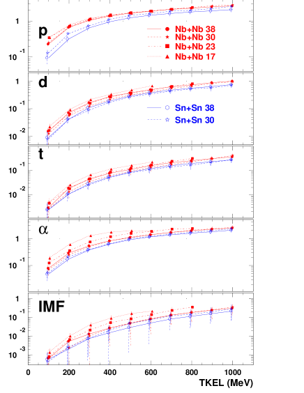
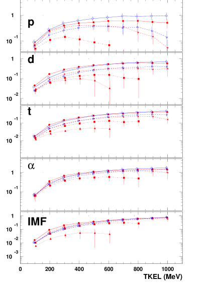
Figure 5: (color online) Experimental, efficiency-corrected evaporative (left) and midvelocity (right) multiplicities of forward-emitted p, d, t, $\alpha$ and IMFs ($Z$=3–7) as a function of TKEL, for ⁹³Nb+⁹³Nb (full symbols) and ¹¹⁶Sn+¹¹⁶Sn (open symbols). Error-bars indicate not statistical errors (they are smaller than the symbols), but rather variations of multiplicity values with analysis procedure (see text). The symbols, with the same meaning as in Fig. 3, are slightly displaced horizontally in order to appreciate the individual error bars at a given TKEL.

Once an estimate of the emission of particles from the PLF has been obtained, the midvelocity component might be derived from the total multiplicities of Fig. 3 using a subtraction procedure Plagnol et al. (1999). However, for an unbiased determination of the evaporative component one should take into account that, due to momentum conservation, the emission of particles – especially of heavy ones – from a source of finite mass produces recoil effects which perturb the velocity of the source itself. Altogether, the net result of a chain of evaporation steps is a superposition of uncorrelated perturbations leading just to a smearing of the original source velocity, with an average null effect. However if the heavy remnant is observed in coincidence with a particle emitted in a specific direction, this fact introduces a correlation between the velocities of the two objects. In particular, if one selects events characterized by the emission of certain particles in a restricted angular range in the source frame, in those events the perturbation of the source velocity will have a non-zero average value.

The requirement that a given particle be emitted in forward direction selects heavy residues which systematically recoil in backward direction. This causes a systematic decrease of the c.m. velocity of the residue (and hence an overestimation of TKEL), while all the other unmeasured or unselected particles contribute only to the smearing of the data. As a consequence, the PLF multiplicities evaluated in a given bin of TKEL do actually pertain to a range of somewhat smaller TKEL values. Or, in other words, they erroneously include some contribution from events belonging to the previous bin (lower TKEL) and miss some contribution from events which are classified in the following one (larger TKEL). It is worth noting that the heavy residue recoils in the (opposite) forward direction when it evaporates particles at angles $\theta_{\mathrm{PLF}}\geq 90^{\circ}$, which then merge with the midvelocity emissions. In this case the c.m. velocity of the residue increases systematically and the resulting TKEL is underestimated. This has to be taken properly into account before subtracting the evaporative component from the total multiplicities.

IV Results

IV.1 Particle multiplicities

The evaporative ($\mathcal{M}_{\mathrm{evap}}$) and midvelocity ($\mathcal{M}_{\mathrm{midv}}$) multiplicities of forward-going particles are presented, as a function of TKEL, in the left and right part of Fig. 5, respectively. The multiplicities refer –with the same symbols– to the same experimental data used for Fig. 3. The vertical scales differ for different particles, but they are the same for the evaporative and midvelocity components of a given particle. It is also worth noting that at 17 A MeV it is not possible to reliably extract the midvelocity multiplicities $\mathcal{M}_{\mathrm{midv}}$ for protons and $\alpha$ particles, because of the overwhelming contribution of the evaporative part.

The error bars of Fig. 5 do not represent statistical errors (which are usually smaller than the symbols). Instead, at each point, they show the maximum variation obtained by choosing a different angular window to select the evaporative component, or by changing the extrapolation to obtain the whole angular distribution, or by switching on/off the recoil corrections. More details are given in Appendix B.

Let us first consider the average multiplicities for the evaporative emission, $\mathcal{M}_{\mathrm{evap}}$. They all display a monotonic increase with increasing TKEL: steeper for the most peripheral collisions, flatter for the less peripheral ones. However, the magnitude of this increase is different for the different particle species. In fact, at small TKEL, the average multiplicities range from a few tenths for protons down to about 10^-3 for tritons or even 10^-4 for IMFs, while at the highest TKEL values considered here the multiplicities are much more leveled off, with 2–3 protons or $\alpha$ particles, as compared to 0.2–0.3 tritons or IMFs. Thus, the entire evolution with TKEL may be comprised within about a decade (protons in the Nb+Nb system), or it may span more than three orders of magnitude (IMFs).

Concerning the dependence on the system size, Fig. 5 shows that, at a given TKEL, the evaporative multiplicities in the ¹¹⁶Sn+¹¹⁶Sn collision (open symbols) are systematically s maller than the corresponding multiplicities in the ⁹³Nb+⁹³Nb collision (full symbols). This holds true for all particle species and at all TKEL values, but it is more clearly visible in the panels for $\alpha$ particles and protons and generally in the lowest TKEL bins. This effect is well reproduced by calculations with the statistical code Gemini Charity et al. (1988) and may be explained by the fact that nuclei produced in the ¹¹⁶Sn + ¹¹⁶Sn reaction, because of the slightly larger initial value of N/Z (1.32 versus 1.27 of 93Nb), get rid of their excitation energy by emitting more neutrons and less charged particles.

As for the beam-energy dependence, at a given TKEL there is a limited sensitivity of $\mathcal{M}_{\mathrm{evap}}$ to this parameter, but nonetheless one can clearly observe, for all particle species, the tendency to rise with decreasing beam energy, a feature that becomes more prominent for heavier particles. For example, in Nb+Nb, the multiplicities are nearly the same for protons at all four bombarding energies, while for $\alpha$ particles and IMFs at small TKEL they rise by about a factor of 1.5–2 from one beam-energy to the next lower one. A possible explanation is that, as already noted, with increasing beam energy the midvelocity emissions draw off an increasing amount of mass and energy from the collision, so that a given TKEL corresponds to smaller excitations of the primary PLFs and hence to lower values of $\mathcal{M}_{\mathrm{evap}}$. Moreover, at high bombarding energies the contact time is shorter and the angular momentum transfer is likely to be smaller so that – in spite of the larger values of the orbital angular momenta in the entrance channel – the primary PLFs may reach lower spin values, an additional fact hindering the evaporation of heavier particles.

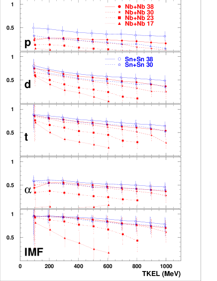
Figure 6: (color online) Ratios of midvelocity-to-total multiplicities of forward-emitted p, d, t, $\alpha$ and IMFs, as a function of TKEL. Symbols have the same meaning as in Fig. 3.

In any case, the variations of $\mathcal{M}_{\mathrm{evap}}$ with bombarding energy are small when compared with the variations (about two orders of magnitude, or more) occurring over the full range of TKEL. Thus, at Fermi energies the variable “TKEL” is still reasonably well correlated with the total amount of particles emitted from the PLF. This observation supports the conclusion Mangiarotti (2003) that, at these beam energies, equal values of TKEL still indicate comparable excitation energies deposited in the PLF (and in the TLF as well).

The midvelocity multiplicities $\mathcal{M}_{\mathrm{midv}}$, displayed in the right part of Fig. 5, present an increase with TKEL similar, at first sight, to that of the evaporative multiplicities $\mathcal{M}_{\mathrm{evap}}$. However, a closer inspection shows that their behavior is in many respects different and to a certain extent complementary. First of all there is a less pronounced rise, the entire evolution with TKEL spanning –for all particles– less than two decades; in some cases the multiplicities seem even to decrease at the highest TKEL. Then, the dependence on the mass size favors the heavier ¹¹⁶Sn+¹¹⁶Sn system, where, at a given TKEL, one generally observes larger $\mathcal{M}_{\mathrm{midv}}$ values, a feature particularly evident for hydrogen isotopes. Finally, at variance with what is observed for $\mathcal{M}_{\mathrm{evap}}$, at a given TKEL value the midvelocity multiplicities show an appreciable increase with increasing beam energy, especially for what concerns the lighter particles.

In order to better appreciate the different dependence of the evaporative and midvelocity multiplicities on the beam energy and TKEL, Fig. 6 presents the ratios of the midvelocity components to the total multiplicities measured in the collisions ⁹³Nb + ⁹³Nb and ¹¹⁶Sn + ¹¹⁶Sn. One observes that generally, for a given beam energy, all ratios decrease with increasing TKEL. Moreover, with decreasing beam energy, the ratios have smaller values and display a faster decrease with increasing TKEL. With the notable exception of the protons and – to a lesser extent – of the $\alpha$ particles, at low TKEL (i.e., in the most peripheral events) the multiplicity ratios tend to reach values as large as 0.8–0.9. This fact confirms that peripheral collisions are the best environment to investigate the phenomenon of the midvelocity emissions with the least contamination from sequential evaporation. This prevalence of the midvelocity particles decreases with increasing centrality of the collision. Comparing the different panels, one sees that protons are mainly produced in evaporative processes and $\alpha$ particles are almost evenly shared between the two mechanisms. On the contrary, the most “exotic” products, i.e., tritons and especially the IMFs, are those which are most specific of the midvelocity emissions: at 38 A MeV, even at the highest TKEL, more than 70% of all emitted IMFs are attributed to the midvelocity component and this percentage rises to almost 100% at small TKEL.

Figure 7: Dependence on beam energy of evaporative (upper panels) and midvelocity multiplicities (lower panels) for forward-emitted p, d, t, $\alpha$ and IMFs ($Z$=3–7) in the ⁹³Nb+⁹³Nb collision. The data correspond to TKEL values of 200 and 400 MeV (left and right panels, respectively).

The different evolution of $\mathcal{M}_{\mathrm{evap}}$ and $\mathcal{M}_{\mathrm{midv}}$ with bombarding energy is shown in Fig. 7 for two TKEL bins in the collision ⁹³Nb + ⁹³Nb. While all evaporative multiplicities stay almost constant, or even show a weak decrease with increasing bombarding energy, the midvelocity multiplicities display a general increasing behavior, more pronounced for the data at higher TKEL.

IV.2 Nature of the emissions

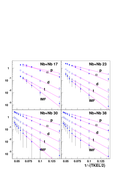
Figure 8: (color online) Multiplicities of PLF-emitted particles as a function of $1/\sqrt{\mathrm{TKEL}/2}$. for ⁹³Nb+⁹³Nb at 17, 23, 30 and 38 A MeV. Lines are linear fits to the logarithm of the multiplicities in the low-energy part of the excitation functions.

In spite of repeated experimental and theoretical efforts over the years, the question about the nature of the mechanism(s) responsible for the observed LCP and IMF emission is still not completely settled.

For what concerns the PLF emissions, it is natural to expect that an evaporation-like de-excitation should be present. Indeed the usual procedure adopted in the literature (see, e.g., Plagnol et al. (1999)), and also in the present paper, for separating the two emission components is based on that working hypothesis. Its validity can be checked by looking at several characteristics of this emission, in comparison with the results of calculations with a statistical evaporation code like Gemini Charity et al. (1988). Hereafter we present some pieces of information which support the hypothesis.

According to statistical theory, the partial decay width associated with a given exit channel should present an exponential dependence on the temperature T of the source (Boltzmann factor, mainly due to the increase of level density with increasing T) of the type: $\Gamma\propto\exp(-{\mathrm{B/T}})$, where B is the barrier associated with that channel. Therefore also the average multiplicities $\mathcal{M}$ of the various evaporated particles may be expected to present a similar exponential dependence on 1/T, or - in a Fermi gas model - on the inverse square root of the excitation energy, $\mathcal{M}\propto\exp(-{\mathrm{c/\sqrt{E^{\star}}}})$, where $c$ is a constant, dependent on the particle species. In order to compare data with these expectations, the first non-trivial task is to estimate the PLF excitation energy. At low bombarding energies (where midvelocity emissions are negligible and TKEL represents the total excitation of the system) and for symmetric systems, TKEL/2 is certainly a good average estimate of the excitation energy of each of the two primary products of a binary reaction. As already noted, with increasing bombarding energy this interpretation becomes more and more questionable due to the increasing relevance of the midvelocity emissions. However, the overall energy balance of the reaction ⁹³Nb+⁹³Nb at 38 A MeV performed in Ref. Mangiarotti et al. (2004) has demonstrated the persistence of an approximately linear correlation between TKEL and the excitation energy of the two primary products. Thus one can suppose that TKEL/2 still represents a measure of the excitation energy of the PLF (and of the TLF as well), although it may be that the scale is no longer a quantitative one, differing at the various bombarding energies. In Fig. 8, the data of the reaction ⁹³Nb+⁹³Nb at the four bombarding energies of 17, 23, 30 and 38 A MeV are presented Mangiarotti (2003) in a semilogarithmic plot as a function of $1/\sqrt{TKEL/2}$. Indeed, the logarithms of the multiplicities of all particles display the same behavior at all bombarding energies, namely a linear one. This fact is put into evidence by the lines, which are fits to the points in the low TKEL region, for each particle species.

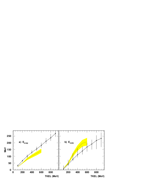
Figure 9: (color online) Average excitation energy of PLF (left) and midvelocity “source” (right) as a function of TKEL for ⁹³Nb+⁹³Nb at 38 A MeV. Uncertainties due to different analyses and assumptions about the n-richness of the midvelocity emissions are indicated by error bars. Dashed lines and shaded areas show estimates and uncertainties of Ref. Mangiarotti et al. (2004).

A more quantitative scale of excitation energy can be estimated following the analysis performed in Ref. Mangiarotti et al. (2004) for the reaction ⁹³Nb+⁹³Nb at 38 A MeV. There the average excitation energy of the primary PLF and of a hypothetical midvelocity “source” was obtained from the total energy balance of the reaction, i.e., by summing up the measured kinetic energies of the respective emitted particles and taking into account the average Q-value for disassembling the system into the final reaction products. For the semiperipheral events of ⁹³Nb+⁹³Nb at 38 A MeV, the excitation energies of the two sources have been re-evaluated with some improvements in the analysis and the results are shown in Fig. 9. The previous estimates of Mangiarotti et al. (2004) (dashed lines) are indicated too, together with their uncertainties (shaded areas) resulting from two rather extreme assumptions about the n-richness of the midvelocity emissions (from N/Z= 1.1 to 1.44). For the present evaluation, the uncertainties due to the same hypotheses on N/Z and to possible variations in the analysis (see Appendix B) are indicated by error bars. Most of the difference with respect to the previous results of Mangiarotti et al. (2004) is due to the use of relativistic kinematics and to the correction for recoil effects.

Figure 10(a) shows the PLF particle multiplicities as a function of the inverse square root of the excitation energy of the primary PLF, $1/\sqrt{E^{\star}_{\mathrm{PLF}}}$. [The first point (TKEL = 100 MeV) is not used here because of the large relative uncertainty of its position on the x-axis, depending on the analysis method (see Appendix B).] When this more appropriate estimate of the excitation energy of the “source” is used, an improved linear behavior is apparent in the logarithmic presentation, as shown by the displayed linear fits to the points. Thus the observed shape of the excitation functions is compatible with a process ruled by statistical laws.

A similar plot, based on the multiplicities calculated with the code Gemini for the decay of an excited ⁹³Nb of spin 30 $\hbar$, is shown in Fig. 10(b). The agreement of the calculations with the experimental data for the PLF-emissions is rather good, thus confirming the evaporative origin of this component.

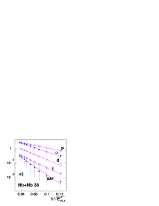
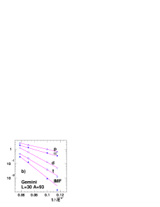
Figure 10: (color online) (a) Multiplicities of PLF-emitted particles as a function of $1/\sqrt{{\mathrm{E}}^{\star}_{\mathrm{PLF}}}$, for ⁹³Nb+⁹³Nb at 38 A MeV, with E${}^{\star}_{\mathrm{PLF}}$ excitation energy (in MeV) of the primary PLF (symbols as in Fig. 8); lines are linear fits to the points. (b) Similar plot, for the decay of a ⁹³Nb nucleus according to Gemini calculations.

No attempt has been made to take into account, in a detailed way, possible changes of mass and spin of the primary PLF with increasing E^⋆, as this was beyond the scope of the comparison. However the relatively weak sensitivity of the calculations to these parameters and the good agreement with the experimental data for the PLF emissions are demonstrated in Fig. 11. In this picture the open symbols show the multiplicities of n, p, d, t, $\alpha$ particles and light IMFs ($Z$=3–7) calculated with the Gemini code for two values (E^⋆= 100 and 200 MeV) of the excitation energy of the evaporating source and for different assumptions on its mass and spin. The full dots show the corresponding experimental multiplicities of PLF-emitted charged particles (neutrons are not measured) for two TKEL bins which, according to the energy balance of Fig. 9(a), correspond to the selected values of E^⋆. Again, the good agreement between experimental data and calculations indicates that the decay of PLFs produced in peripheral and semiperipheral collisions is compatible with the usual evaporation of an excited nucleus at normal density, at least for what concerns the first 3–4 fm of overlap (see Appendix A). So, at variance with the claims of other authors Milazzo et al. (2002), in order to reproduce our data there is no need to resort to models (like SMM Bondorf et al. (1995)) which describe the fragmentation of an expanding diluted nucleus (typically at one third of normal density). Possibly, the reason is that the events analyzed by the cited authors are less peripheral (indeed their estimated PLF excitation energies are around 4–5 A MeV, i.e., higher than ours) and correspond to a rather particular event selection (at least 3 IMFs) and not to the bulk of the collisions as in our case. It has also been verified that, as expected for an equilibrated emission, the velocity spectra of the emitted LCPs have approximately Maxwellian shapes with slope parameters of the order of 2–5 MeV, depending on the selected TKEL value.

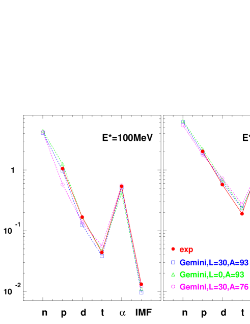
Figure 11: (color online) Multiplicities of light particles and light IMFs (Z=3–7) evaporated from the PLF in ⁹³Nb+⁹³Nb at 38 A MeV, for an estimated PLF excitation energy of 100 and 200 MeV (left and right panel, respectively). Experimental data (full dots) are compared with Gemini calculations (open symbols) with different mass and spin of the source; for the calculations also the neutron multiplicities are shown.

Finally, the lower part of Fig. 12 shows the average N/Z ratio of hydrogen isotopes emitted by the PLF in the reaction ⁹³Nb+⁹³Nb at 38 A MeV (full dots). This ratio increases with TKEL from 0.1 to about 0.4 and is compatible with the results of Gemini calculations for the decay of a ⁹³Nb nucleus at normal density with the appropriate excitation energy obtained from Fig. 9(a).

For what concerns the midvelocity component, some characteristic aspects (like, e.g., the emission pattern of LCPs and IMFs, the space-time extension of the “source” and its associated energy Montoya et al. (1994); Plagnol et al. (1999); Piantelli et al. (2002); De Filippo et al. (2005); Hudan et al. (2005)) have been already investigated in the past. However, very different hypotheses have been proposed for the underlying mechanism, ranging from fully dynamical processes (like, e.g., surface instabilities in the non-spherical, transient shapes of the interacting system Baran et al. (2004)) to purely statistical ones (like, e.g., a proximity-enhanced statistical decay of PLF and TLF in the external inhomogeneous Coulomb field of the other reaction partner Botvina et al. (1999); Botvina and Mishustin (2001)), although it cannot be excluded that more than one mechanism contributes to the observed phenomena Piantelli et al. (2002).

The average N/Z ratio of the hydrogen isotopes in the midvelocity component is shown by the open dots in the upper part of Fig. 12, again for the reaction ⁹³Nb+⁹³Nb at 38 A MeV. This ratio has now much larger values (from 0.6 to about 1.0), thus indicating a substantial difference between the emissions from the PLF and those at midvelocity. This may be an indication of neutron enrichment at midvelocity, as proposed on the basis of the emission of complex particles Dempsey et al. (1996); Łukasik et al. (1997); Plagnol et al. (1999); Larochelle et al. (2000); Milazzo et al. (2002); Piantelli et al. (2002), or it may be somehow related to the reduced size of the “source” and hence to its higher energy concentration, as indicated in Mangiarotti et al. (2004).

The energy deposited in the matter at midvelocity, $E^{\star}_{\mathrm{midv}}$, estimated from the energy balance of Fig. 9(b), is used in Fig. 13 to present also the midvelocity multiplicities in a logarithmic plot as a function of $1/\sqrt{E^{\star}_{\mathrm{midv}}}$: to our knowledge, this is the first time that midvelocity multiplicities are presented in this way. (Here too, the first point at TKEL = 100 MeV has not been used.) First of all, we want to point out some remarkable differences between the midvelocity emissions of Fig. 13 and the PLF emissions of Fig. 10(a). For example, all midvelocity multiplicities are compressed within about one decade (note the different horizontal and especially vertical scales of the two figures) and consequently their slopes are all sizably flatter. Even more striking is the fact that the relative abundances of the emitted particles are different, with remarkable inversions between protons and $\alpha$ particles and between tritons and IMFs.

Figure 12: Average value of N/Z for evaporative (full dots) and midvelocity (open dots) emission of Hydrogen as a function of TKEL in ⁹³Nb+⁹³Nb at 38 A MeV. Dashed lines are the results of calculations with the code Gemini.

In this presentation as a function of $1/\sqrt{E^{\star}_{\mathrm{midv}}}$, one observes a linear correlation also for the midvelocity emissions, as demonstrated by the linear fits to the points, but no easy interpretation is at hand. For a different process, namely multifragmentation in central collisions, it was argued Moretto et al. (1993) that such a linear behavior (called thermal scaling) would be the proof of the statistical, sequential decay of the “source” (the role of dynamics being relegated to its formation), but this conclusion is amply disputed. In fact, very different models proved able to reproduce a similar behavior, and no general consensus is reached on aspects like the appropriate treatment of the data and estimation of the source temperature, the sequentiality or simultaneity of the process, the role of fluctuations and correlations (see, e.g., Botvina and Gross (1995); Elliott et al. (2000); Beaulieu et al. (2001) and references therein). Although the linear behavior in itself may be suggestive of a thermal process, its mere observation is not a proof and one actually expects that in peripheral collisions the dynamics should play a much more important role than in central collisions.

As a last point, it is worth noting that these striking differences between evaporative and midvelocity multiplicities give strong support to and demonstrate the effectiveness of the separation procedure outlined in Sec. III.5, which has been used to disentangle the two components.

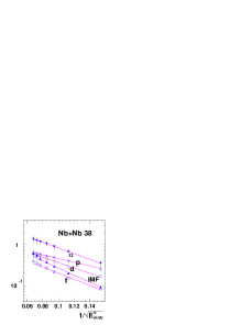
Figure 13: (color online) Semilogarithmic plot of midvelocity particle multiplicities as a function of $1/\sqrt{E^{\star}_{\mathrm{midv}}}$ for Nb+Nb at 38 A MeV (symbols as in Fig. 8). $E^{\star}_{\mathrm{midv}}$ is the excitation energy of the emitting “source”, lines are fits to the points.

V Summary and Conclusions

The symmetric collisions ⁹³Nb + ⁹³Nb at 17, 23, 30 and 38 A MeV and ¹¹⁶Sn+¹¹⁶Sn at 30 and 38 A MeV have been investigated using the Fiasco setup, a low-threshold multidetector covering a large fraction of the forward solid angle.

The present analysis is focused on peripheral and semiperipheral events resulting from binary or quasi-binary reaction processes. They are characterized by the presence in the exit channel of two heavy remnants, which can be identified as the projectile- and target-like fragments. These binary or quasi-binary processes are found to exhaust more than half of the expected total reaction cross section at all the investigated beam energies.

The kinematic variable TKEL has been used for selecting event samples corresponding, on average, to decreasing values of the impact parameter. It is worth stressing that TKEL, which at low bombarding energies represents a good estimate of the total excitation of the colliding nuclei, looses such a physical meaning at Fermi energies and therefore it is used here only as an ordering parameter.

The average multiplicities $\mathcal{M}$ of light charged particles and intermediate mass fragments with $3\leq Z\leq 7$ have been obtained as a function of TKEL for all the investigated systems. The data have been evaluated in a range of TKEL values which is estimated to roughly correspond to the outermost 30% of the impact parameter range leading to nuclear interaction. The emission pattern of these particles in the ($v_{\,\parallel}$,$v_{\,\perp}$) plane – the velocity components being referred to the PLF - TLF separation axis in the c.m. reference system – clearly shows the presence of two components, one representing an emission from the excited PLF (and TLF) and a second one at midvelocity, i.e., at velocities intermediate between that of PLF and TLF. A careful analysis of the shape of the angular distribution in the reference frame of the PLF has been applied in order to distinguish and estimate the multiplicities of particles emitted by the PLF and, by a subtraction procedure, those of the particles emitted in the midvelocity region. Correction have been applied to take into account the efficiency of the setup, as well as physical effects due to spin and recoil of the emitting nuclei.

Both emission components increase with increasing TKEL (i.e., decreasing impact parameter), although their behavior is different. More “exotic” particles (like tritons, IMFs and to a lesser extent deuterons) are characteristic of midvelocity processes in the most peripheral events, where they outnumber the emissions from PLF. Moreover, for a fixed TKEL, the midvelocity emissions present a clear increase with increasing beam energy, while the emissions from PLF show little dependence on the beam energy.

The dependence of PLF emissions on the estimated excitation energy of the PLF follows that expected for a decay mechanism governed by a barrier and is well described within statistical models. In fact, calculations with the statistical code Gemini well reproduce all experimental features, including the slopes of the excitation function, the relative and absolute abundances of the various particle species and also the isotopic composition of Hydrogen particles. Thus, at least for the peripheral and semiperipheral collisions, the decay of the PLF (and TLF) is in many aspects compatible with the usual evaporation from an excited nucleus at normal density.

Surprisingly, also the midvelocity emissions display a similar type of dependence on the amount of energy which is localized in the hypothetical midvelocity “source”. However, this mechanism is quite different from the usual evaporation, as it is shown by the inversion in the relative abundance of the emitted particles and by the tendency to emit more n-rich light particles. Indeed, the emission pattern observed in this work and in previous ones Piantelli et al. (2002), clearly demonstrates that this hypothetical “source” is not a simple spherical one, sitting at midvelocity and isotropically emitting particles; on the contrary, in order to reproduce the observed emission patterns, one needs a more complex “source”, extended both in space and time. For a satisfactory explanation of its characteristic features, one probably needs a dynamic description of the collision Baran et al. (2004), but its successive decay seems to possess some features reminiscent of a statistical process.

Appendix A Impact parameter estimation

Various experimental variables are used in literature for estimating how central or peripheral a collision is and for sorting the measured events in (nearly) homogeneous samples. Among the variables related only to the main reaction partners, an often used one is the secondary charge $Z_{\mathrm{sec}}$ of the PLF residue (at low bombarding energies or for quasi-peripheral events) or the charge of the heaviest fragment $Z_{\mathrm{max}}$ (at higher energies or for more central collisions): in fact, on average, the lighter this charge, the more violent and central the collision is likely to be Djerroud et al. (2001). Such non-kinematic variables may be used for studying kinematic aspects of particles (like, e.g., their angular distributions), but they are not equally well suited for studying multiplicities. Because of the finite (and not too large) total charge of the system, spurious correlations may appear.

In order to avoid this problem, it is preferable to sort the data according to a kinematical variable, such as the secondary velocity $v^{\;\mathrm{Lab}}_{\;\mathrm{PLF}}$ of the PLF in the laboratory reference system Yanez et al. (2003), or the relative velocity $v_{\;\mathrm{rel}}$ of the two main reaction products, or the energy loss per nucleon $\epsilon^{\star}$ of a binary collision Métivier et al. (2000). In this paper we have adopted TKEL, as defined in Eq. (1). In case of a binary process with frozen initial mass asymmetry one expects to find a good correspondence between all these kinematic variables, but if the mass asymmetry in the exit channel is allowed to change, then TKEL has the advantage of explicitly taking into account these variations.

The experimental correlation of TKEL with $v_{\;\mathrm{rel}}$ and $v^{\;\mathrm{Lab}}_{\;\mathrm{PLF}}$ for the data of ⁹³Nb + ⁹³Nb at 38 A MeV is shown in Fig. 14(a) and (b), respectively. The first correlation, TKEL–$v_{\;\mathrm{rel}}$, is extremely narrow in the whole considered range: this is little surprise, since in symmetric collisions most binary exit channels have nearly the same reduced mass, so that TKEL is approximately proportional to $v_{\;\mathrm{rel}}^{2}$ [see Eq. (1)]. The next correlation, TKEL vs $v^{\;\mathrm{Lab}}_{\;\mathrm{PLF}}$, is narrow at low TKEL, but tends to become wider with increasing inelasticity of the collision. Finally, Fig. 14(c) also shows the correlation of TKEL with $Z_{\mathrm{sec}}$: the two variables are well correlated but with rather large fluctuations.

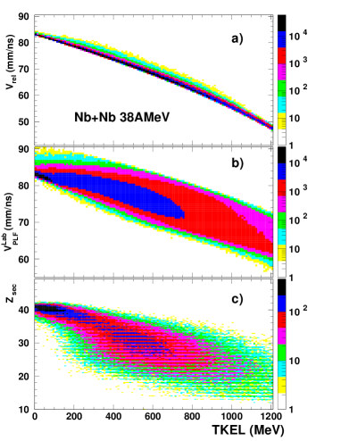
Figure 14: (color) Experimental correlations between the kinematic variable TKEL [see Eq. (1)] and (a) relative PLF-TLF velocity; (b) lab-velocity of the PLF; (c) secondary charge of the PLF. Data refer to ⁹³Nb + ⁹³Nb at 38 A MeV.

The usage of TKEL as an impact parameter estimator is supported by the kinematic analysis of events generated with the Quantum Molecular Dynamics (QMD) code Chimera Łukasik and Majka (1993). The velocity vectors of the two main fragments produced by such QMD calculations were used to deduce the variable TKEL, just with the same kinematic procedure used for the experimental data: the result of this analysis shows a nice correlation between impact parameter and TKEL Piantelli (2001). The average value of the obtained TKEL, plotted as a function of the impact parameter used as input to the calculations, is shown in the upper part of Fig. 15 for the investigated reactions (except for the 17 A MeV case, because at such a low bombarding energy the QMD approach seems hardly applicable). As expected, there is a monotonic increase of TKEL when the impact parameter is decreased starting from the grazing value $b_{\mathrm{graz}}$. Less obvious is the finding that, for a given system, at large impact parameters the correlations are almost independent of the beam energy. The model suggests that, at different bombarding energies, peripheral events sampled in the same TKEL bins may correspond to collisions with roughly the same impact parameter. As the collisions become less and less peripheral, the curves progressively separate and bend down, as they approach – at different TKEL values – the limit of their respective available energy in the c.m. system. Concerning the comparison of the two systems, for ¹¹⁶Sn + ¹¹⁶Sn the correlations begin at a larger value of b, as might have been expected, and proceed almost parallel to those of the lighter system ⁹³Nb + ⁹³Nb.

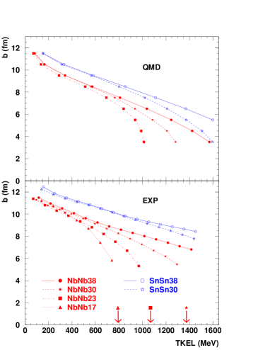
Figure 15: (color online) Upper panel: average correlation between impact parameter and the kinematical variable TKEL for events generated by the QMD code Chimera Łukasik and Majka (1993). Lower panel: average correlation between impact parameter and TKEL obtained from the integration of the experimental reaction cross section for ⁹³Nb+⁹³Nb at 17, 23, 30, 38 A MeV and ¹¹⁶Sn+¹¹⁶Sn at 30, 38 A MeV; arrows indicate the c.m. available energies which are within the displayed energy range. Lines are just an aid to guide the eye.

As an alternative, one can perform an association of TKEL with impact parameter using a method already applied in Ref. Stefanini et al. (1995) and based on a refinement of an even older recipe Schröder et al. (1978). The basic hypothesis is that there is a good average correlation between decreasing impact parameter and macroscopic behavior of the reaction products in terms of scattering angle and kinetic energy dissipation. So one can try to follow the evolution of the reaction from the two-dimensional plot $d^{\,2}\sigma/d(\theta_{c.m.})d({\mathrm{TKEL}})$, the so-called Wilczynski-plot Wilczynski (1973), and empirically determine – on average – an impact parameter scale by means of an integration of the reaction cross section, starting from the elastic region, going over to the quasi-elastic region and then down into the deeply inelastic region; events leading to fusion or to several heavy fragments are assumed to be located at the lower end of the impact parameter scale.

In practice, during our experiment, events from a minimum bias trigger (“singles”, requiring a number M$\geq$1 of hits in the gas detectors) were acquired at a reduced rate, together with rarer events from more selective triggers (requiring higher-fold hits). For the four most forward gas detectors, “clean” angular distributions can be obtained for these minimum-bias events by selecting appropriate equal windows in the azimuthal angle and further requiring that the time-of-flight be compatible with that of elastically scattered projectiles. The so obtained angular distributions nicely reproduce the $1/\sin^{4}(\theta_{c.m.}/2)$ shape expected for the Rutherford scattering of pointlike charges, until the region near the grazing angle is reached. The method is very sensitive; small differences in the rates of the four most forward gas detectors, have been attributed to a misalignment (generally less than one tenth of a degree) of the beam with respect to the optical axis and were used to correct the polar angles. For each of the investigated reactions, a simultaneous fit of the Rutherford formula to the angular distributions of the four gas detectors has been used to estimate the conversion factor from counts to millibarns, with an uncertainty below a few percent.

The procedure is then illustrated with the help of Fig. 16, where the correlation $d^{2}\sigma/d\theta_{\mathrm{c.m.}}d\mathrm{TKEL}$ for binary events is sketched together with its total projection $d\sigma/d\mathrm{TKEL}$ (on the left) and a projection $d\sigma/d\theta_{\mathrm{\,c.m.}}$ of the elastic and quasi-elastic region (on the top). The region $A$ is dominated by elastic scattering (which is responsible for the large peak around TKEL$\approx$0 in the projection on the left), while regions $B$ (still at TKEL$\approx$0, but beyond the grazing angle $\theta^{\mathrm{graz}}_{\mathrm{\,c.m.}}$) and $C$ are populated by reactions. The two-body cross sections of Table 2 have been obtained by integrating the efficiency corrected experimental yields in regions $B$ and $C$ (with a small correction to take into account the quasi-elastic cross section lying below the elastic ridge in region $A$), while the three-body cross sections come from the lower part of region $C$ only.

The correlation between impact parameter $b$ and TKEL is obtained by filling the triangle-shaped distribution $d\sigma/d\,b$ (upper part of Fig. 16) in successive steps. Starting from a value of $\theta_{\mathrm{\,c.m.}}$ still in the elastic region (which is uniquely related to impact parameter by Rutherford scattering), one integrates the measured cross section at larger angles (remaining part of the region $A$ and region $B$), thus determining a new impact parameter value, which is the first point in the experimental correlations [see Fig. 15(b)]. Now one proceeds towards smaller and smaller impact parameters by integrating the measured cross section for more and more inelastic events (in region $C$).

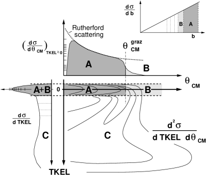
Figure 16: Sketch of the cross section integration

In a “sharp cut-off” picture, each successive integrated piece of cross section is used to completely fill the next (to the left) slice of the triangle $d\sigma/d\,b$, thus determining the next point of correspondence between impact parameter $b$ and TKEL. Of course, for this procedure to work reasonably, what must be integrated is the total reaction cross section. For the present work, focused on peripheral collisions, this means that it is necessary to obtain:

• a good quantitative measurement of the most representative exit channels of the reaction (i.e., two-body and, to a lesser extent, three-body events);

• a good correction for the inefficiencies of the setup (“experimental filter”);

• a smooth transition, without detection gaps, from the elastic to the inelastic events (i.e., not too complicated triggers and good efficiency for quasi-elastic events).

The results for the investigated reactions are presented in the lower panel of Fig. 15. Qualitatively there is a good agreement with the results of the QMD estimates, as the same main features are well reproduced: (1) There is the same monotonic decrease of $b$ with increasing TKEL. (2) For very peripheral collisions the correlations are almost independent of the beam energy, while they tend to separate at smaller impact parameters. (3) For ¹¹⁶Sn + ¹¹⁶Sn the curves are displaced by an almost constant value of about 1 fm to larger impact parameters.

For each curve, the first point – that at the highest $b$ – is the most critical one and it is estimated to be affected by an overall uncertainty of the order of 1 fm (due to corrections of misalignment of the beam axis, fitting with Rutherford scattering, integration of elastic cross section, matching of elastic and inelastic events). Being the curves obtained by successive integrations of the cross section, the errors are strongly correlated and the uncertainty on the first point propagates to all other points; in other words, if the first point needed to be moved up or down, all the others would move almost rigidly in the same direction. Considering that the Fiasco setup has been developed and optimized for peripheral reactions, this impact parameter determination becomes less reliable when the collisions become more central In fact, one may start missing some relevant exit channel and, in turn, this progressive underestimation of the total reaction cross section may cause the impact parameter to decrease too slowly with TKEL. Indeed, this might explain why, at large TKEL and especially for larger beam energies, the experimental curves shown in the lower panel of Fig. 15 do not bend downwards as much as the QMD calculations.

In the TKEL ranges used for the evaluation of the multiplicities presented in this paper (TKEL $\leq$ 600 and 800 MeV for Nb+Nb at 17 and 23 A MeV, respectively; $\leq$1000 MeV in all remaining cases) the binary channel accounts for about 2.0–2.2 barn in the ⁹³Nb + ⁹³Nb collisions and about 1.9 barn in the ¹¹⁶Sn + ¹¹⁶Sn collisions (corresponding to $\sim$ 40–50% and $\sim$ 35% of $\sigma_{\mathrm{reac}}^{\mathrm{\,calc}}$, respectively), with an uncertainty of about 200–300 mb. The applied restriction on the ratio of the two c.m. velocities (0.4 $\leq v^{\mathrm{c.m.}}_{\mathrm{PLF}}/(v^{\mathrm{c.m.}}_{\mathrm{PLF}}+v^{\mathrm{c.m.}}_{\mathrm{TLF}})\leq$ 0.6) cuts less than 5% of the considered cross section and is appreciable only in the last considered TKEL bin. From the integration of the experimental cross section it is estimated that the presented multiplicities refer approximately to the outermost third of the impact parameter range ($b^{\mathrm{exp}}$ / $b_{\mathrm{graz}}^{\mathrm{calc}}\geq$ 60–70%). In this region, choosing the same TKEL bin allows to compare results at roughly the same impact parameter if the system is fixed and only the beam energy is varied, while it is confirmed that there is a shift of about 1 fm between the estimated impact parameters for the two systems ⁹³Nb + ⁹³Nb and ¹¹⁶Sn + ¹¹⁶Sn.

Appendix B Dependence on the analysis method

In order to estimate the uncertainties which may affect the determination of the average evaporative and midvelocity multiplicities ($\mathcal{M}_{\mathrm{evap}}$ and $\mathcal{M}_{\mathrm{midv}}$, respectively), the data have been analyzed by using slightly different procedures for separating the total multiplicities into these two components. More specifically, somewhat different choices have been taken at three important points of the analysis and the induced variations have been considered as representative of the sensitivity of the results to different evaluation procedures. The three points are

• the angular range (in the PLF frame) used to estimate the evaporative component,

• the successive extrapolation of the angular distribution to the whole range 0^∘–180^∘,

• the corrections for recoil effects.

As for point (a), besides the adopted range of 0^∘–45^∘, a more conservative one (0^∘–30^∘) has been considered, as well as the range 0^∘–90^∘, which is often used in the literature. As already discussed with regard to Fig. 4, this last choice pays the advantage of estimating the whole angular distribution by means of a simple reflection around 90^∘ [without the extrapolation of point (b)] with the disadvantage that the evaporative component may be contaminated by the tail of the midvelocity emission.

The extrapolation at point (b) requires some hypothesis on the spin value of the evaporating source and its misalignment during the decay, while for a zero-spin source one expects a roughly $\cos{\theta_{\mathrm{\;PLF}}}$-shaped angular distribution $d\sigma/d\theta_{\mathrm{\;PLF}}$ (although recoil effects may somewhat distort it). So the considered alternatives are an analytical extrapolation with the $\cos{\theta_{\mathrm{\;PLF}}}$ shape and a numerical one, obtained with a Monte Carlo simulation which assumes a non-zero spin value (rising with TKEL from 0 $\hbar$ to 40 $\hbar$) and takes into account the progressive spin misalignment along the evaporation chain.

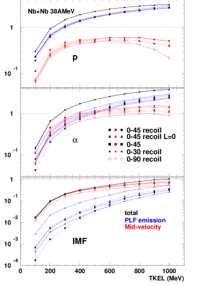
Figure 17: (color) Total (black), evaporative (blue) and midvelocity (red) multiplicities for p, $\alpha$ and IMFs (upper, middle and lower panels, respectively) in ⁹³Nb+⁹³Nb at 38 A MeV. The results of the analysis adopted in the paper (full dots) are compared with those obtained from slightly different analysis procedures (see text).

Figure 17 shows the differences which are typically obtained, by taking as an example the evaporative (blue color) and midvelocity (red color) multiplicities of p, $\alpha$ and IMFs in the reaction ⁹³Nb + ⁹³Nb at 38 A MeV (the three cases correspond to dominant evaporation, comparable components and dominant midvelocity emission, respectively); the black curves show the corresponding total multiplicities. The reference (shown by full dots) is always the analysis with the choices adopted in this paper, namely evaporation in the angular range 0^∘–45^∘, extrapolation – based on Monte Carlo simulations – for non-zero spin source and applied corrections for recoil effects. Variations are then made one at a time: either a zero-spin source is assumed (triangles), or the recoil corrections are switched off (squares), or the angular range is reduced to 0^∘–30^∘ (stars) or even enlarged to 0^∘–90^∘ (open dots).

Being the decomposition between $\mathcal{M}_{\mathrm{evap}}$ and $\mathcal{M}_{\mathrm{midv}}$ obtained with a subtraction procedure, these different choices induce larger relative variations in the weaker component: thus, in the evaporative component they are largest for the IMFs (which are predominantly emitted at midvelocity) and, in the midvelocity component, they are rather large for protons at 38 A MeV and even larger – this time for all particles – at the lowest bombarding energies (where evaporation dominates).

In general one can observe that:

• The more conservative angular range 0^∘–30^∘ gives values of $\mathcal{M}_{\mathrm{evap}}$ ($\mathcal{M}_{\mathrm{midv}}$) which are just slightly smaller (larger) than those obtained with 0^∘–45^∘. Only for IMFs there is a sizable reduction (about -30%) of the already quite small $\mathcal{M}_{\mathrm{evap}}$ component (while the corresponding increase of $\mathcal{M}_{\mathrm{midv}}$ is negligible).

• With the commonly used procedure of estimating the evaporation by taking twice the particles emitted in 0^∘–90^∘, one systematically overestimates $\mathcal{M}_{\mathrm{evap}}$ (and hence underestimates $\mathcal{M}_{\mathrm{midv}}$), for all particles and at all bombarding energies. For protons, the variation is negligible on $\mathcal{M}_{\mathrm{evap}}$ and small but sizable on $\mathcal{M}_{\mathrm{midv}}$ (especially at high TKEL); for $\alpha$ the effect is of the order of 30–40% and comparable on both components; for IMFs the effect is huge (about a factor of 2–3) on the weak $\mathcal{M}_{\mathrm{evap}}$ component and much smaller – but still sizable, about 20–30% – on the dominating $\mathcal{M}_{\mathrm{midv}}$. Indeed, for IMFs this procedure gives the largest of all considered variations.

• Extrapolating the angular distribution of evaporated particles with a $\cos{\theta_{\mathrm{\;PLF}}}$ shape generally overestimates $\mathcal{M}_{\mathrm{evap}}$ (and underestimates $\mathcal{M}_{\mathrm{midv}}$). However, at small TKEL (where the spin is likely to be small), it produces really negligible variations in all cases. At large TKEL, there is a moderate effect (of the order of 10–20%) only on the weaker component.

• As explained in Sec. III.5, applying no recoil correction causes an overestimation of TKEL, namely a given bin erroneously includes some events (which should actually be classified in a bin at lower TKEL) and misses others (which get classified in another bin at larger TKEL). The net effect of this gain and loss is determined by the TKEL dependence of the experimental particle yield, i.e., yield of measured events times event multiplicity for that particle). The rise of all multiplicities is steepest at small TKEL and tends to flatten at large TKEL, while the measured event yield doesn’t change more than a factor of two over the whole TKEL range. Therefore the effect of the recoil correction is largest at small TKEL, where it determines an increase of $\mathcal{M}_{\mathrm{evap}}$ – of course larger for heavier particles – from 10–20% for protons to a factor of about 2 and 3 for $\alpha$ particles and IMFs, respectively (the corresponding decrease of $\mathcal{M}_{\mathrm{midv}}$ is about 70% for protons, a factor of 2 for $\alpha$ and negligible for IMFs).

In the Nb+Nb system at 38 A MeV, the effects of the considered analysis variations are most visible in the PLF-multiplicities of IMFs at large beam energies, and in the midvelocity multiplicities of LCPs at low beam energies and large TKEL. For all investigated reactions, these effects are schematically represented by the error bars in Figs. 5 and 6 and they should be kept in mind when comparing the results of different experiments obtained with different analysis procedures.

References

- Łukasik et al. (1997) J. Łukasik et al., Phys. Rev. C 55, 1906 (1997).
- Plagnol et al. (1999) E. Plagnol et al. (INDRA collaboration), Phys. Rev. C 61, 014606 (1999).
- Piantelli et al. (2002) S. Piantelli, L. Bidini, G. Poggi, M. Bini, G. Casini, P. R. Maurenzig, A. Olmi, G. Pasquali, A. A. Stefanini, and N. Taccetti, Phys. Rev. Lett. 88, 052701 (2002).
- Milazzo et al. (2002) P. M. Milazzo et al., Nucl. Phys. A703, 466 (2002).
- Mangiarotti et al. (2004) A. Mangiarotti et al., Phys. Rev. Lett. 93, 232701 (2004).
- Stefanini et al. (1995) A. A. Stefanini et al., Z. Phys. A 351, 167 (1995).
- Bowman et al. (1993) D. R. Bowman et al., Phys. Rev. Lett. 70, 3534 (1993).
- Montoya et al. (1994) C. P. Montoya et al., Phys. Rev. Lett. 73, 3070 (1994).
- Tõke et al. (1996) J. Tõke et al., Phys. Rev. Lett. 77, 3514 (1996).
- Dempsey et al. (1996) J. F. Dempsey et al., Phys. Rev. C 54, 1710 (1996).
- Baran et al. (2004) V. Baran, M. Colonna, and M. Di Toro, Nucl. Phys. A730, 329 (2004).
- Botvina et al. (1999) A. S. Botvina, M. Bruno, M. D’Agostino, and D. H. E. Gross, Phys. Rev. C 59, 3444 (1999).
- Botvina and Mishustin (2001) A. S. Botvina and I. N. Mishustin, Phys. Rev. C 63, 61601R (2001).
- Casini et al. (1993) G. Casini et al., Phys. Rev. Lett. 71, 2567 (1993).
- Bocage et al. (2000) F. Bocage et al. (INDRA collaboration), Nucl. Phys. A676, 391 (2000).
- De Filippo et al. (2005) E. De Filippo et al., Phys. Rev. C 71, 044602 (2005).
- Di Toro et al. (2006) M. Di Toro, A. Olmi, and R. Roy, Eur. Phys. J. A (2006), (to be published).
- Hudan et al. (2005) S. Hudan et al., Phys. Rev. C 71, 054604 (2005).
- Durand (1998) D. Durand, Nucl. Phys. A630, 52c (1998).
- Bini et al. (2003) M. Bini et al., Nucl. Instrum. Methods Phys. Res. A 515, 497 (2003).
- Piantelli (2001) S. Piantelli, Ph.D. thesis, Florence University (2001).
- Mangiarotti (2003) A. Mangiarotti, Ph.D. thesis, Florence University (2003).
- Bass (1980) R. Bass, Nuclear Reactions with Heavy Ions, Texts and Monographs in Physics (Springer Verlag, 1980).
- Charity et al. (1991) R. J. Charity et al., Z. Phys. A 341, 53 (1991).
- Casini et al. (1989) G. Casini, P. R. Maurenzig, A. Olmi, and A. A. Stefanini, Nucl. Instrum. Methods Phys. Res. A 277, 445 (1989).
- Immè et al. (March 1993) G. Immè et al., in Proc. Workshop on Detector and Instrumentation, Acireale (Catania) (March 1993).
- Sfienti et al. (2004) C. Sfienti, V. Baran, M. De Napoli, G. Immé, G. Raciti, E. Rapisarda, S. Rascuná, and L. Spezzi, Nucl. Phys. A734, 528 (2004).
- Schröder and Huizenga (1977) W. U. Schröder and J. R. Huizenga, Ann. Rev. Nucl. Sci. 27, 465 (1977).
- D’Agostino et al. (1999) M. D’Agostino et al., Nucl. Phys. A650, 329 (1999).
- (30) A. Mangiarotti et al., to be published.
- Døssing (1981) T. Døssing, Nucl. Phys. A357, 488 (1981).
- Moretto et al. (1981) L. G. Moretto, S. K. Blau, and A. J. Pacheco, Nucl. Phys. A364, 125 (1981).
- Charity et al. (1988) R. J. Charity et al., Nucl. Phys. A483, 371 (1988).
- Bondorf et al. (1995) J. P. Bondorf, A. S. Botvina, A. S. Iljinov, I. N. Mishustin, and K. Sneppen, Phys. Rep. 257, 133 (1995).
- Larochelle et al. (2000) Y. Larochelle et al., Phys. Rev. C 62, 51602R (2000).
- Moretto et al. (1993) L. G. Moretto, D. N. Delis, and G. J. Wozniak, Phys. Rev. Lett. 71, 3935 (1993).
- Botvina and Gross (1995) A. S. Botvina and D. H. E. Gross, Phys. Lett. B344, 6 (1995).
- Elliott et al. (2000) J. B. Elliott et al., Phys. Rev. Lett. 85, 1194 (2000).
- Beaulieu et al. (2001) L. Beaulieu et al., Phys. Rev. C 63, 031302 (2001).
- Djerroud et al. (2001) B. Djerroud et al., Phys. Rev. C 64, 034603 (2001).
- Yanez et al. (2003) R. Yanez et al., Phys. Rev. C 68, 011602 (2003).
- Métivier et al. (2000) V. Métivier et al. (INDRA collaboration), Nucl. Phys. A672, 357 (2000).
- Łukasik and Majka (1993) J. Łukasik and Z. Majka, Acta Phys. Pol. B24, 1959 (1993).
- Schröder et al. (1978) W. U. Schröder, J. R. Birkelund, J. R. Huizenga, K. L. Wolf, and V. E. Viola Jr., Phys. Rep. 45, 301 (1978).
- Wilczynski (1973) J. Wilczynski, Phys. Lett. B47, 484 (1973).