Experimental determination of the complete spin structure for
$\bar{p}p\rightarrow\bar{\Lambda}\Lambda$ at $p_{\bar{p}}=1.637$ GeV/c

Abstract

The reaction $\bar{p}p\rightarrow\bar{\Lambda}\Lambda\rightarrow\bar{p}\pi^{+}p\pi^{-}$ has been measured with high statistics at a beam momentum of $p_{\bar{p}}=1.637$ GeV/c. The use of a transversely-polarized frozen-spin target combined with the self-analyzing property of $\Lambda/\bar{\Lambda}$ decay allows access to unprecedented information on the spin structure of the interaction. The most general spin-scattering matrix can be written in terms of eleven real parameters for each bin of scattering angle, each of these parameters is determined with reasonable precision. From these results all conceivable spin-correlations are determined with inherent self-consistency. Good agreement is found with the few previously existing measurements of spin observables in $\bar{p}p\rightarrow\bar{\Lambda}\Lambda$ near this energy. Existing theoretical models do not give good predictions for those spin-observables that had not been previously measured.

I Introduction

Measurements have been made of the $\bar{p}p\rightarrow\bar{\Lambda}\Lambda$ reaction on a transversely polarized frozen-spin target. An analysis is presented of data taken at the Low Energy Antiproton Ring (LEAR) at CERN, Geneva at $p_{\bar{p}}=1.637$ GeV/c corresponding to a center-of-mass energy which is 78 MeV above $\bar{\Lambda}\Lambda$ threshold.

This experiment, carried out by the PS185 collaboration, expands upon a series of $\bar{Y}Y$ production and related experiments old_PS185 ; Horsti ; threshold ; recent_PS185 which have previously been performed by this collaboration using the same detector system. These covered wide-ranging kinematics from very near threshold to higher energies at which the larger cross section allowed high-statistics studies to be made.

Spin observables have long been of interest in strangeness-production reactions in part because of the characteristic strong polarization produced. The hyperons in the final state (the word ’hyperon’ will be used loosely to include anti-hyperons) lend themselves to study of spin dynamics because of the self-analyzing power of mesonic hyperon decay. Thus, even before the introduction of initial-state polarization in these studies, the PS185 collaboration has been able to greatly expand the world’s supply of data on spin observables, especially for $\bar{p}p\rightarrow\bar{\Lambda}\Lambda$. In particular, final-state polarization components of both hyperons and correlations of all spin components of $\Lambda$ and $\bar{\Lambda}$ were accurately measured in addition to differential cross sections.

The wealth of data produced by PS185 old_PS185 ; Horsti ; threshold ; recent_PS185 excited a great deal of theoretical activity MEX_old ; MEX_QG ; MEX_pred ; QG_old ; QG_pred ; other_theory with several models enjoying reasonable success in fitting the observations. Two distinct theoretical approaches, meson-exchange [MEX] and quark-gluon [QG] inspired models, have been used successfully to fit the $\bar{p}p\rightarrow\bar{\Lambda}\Lambda$ data despite being based on fundamentally different reaction dynamics.

Several authors MEX_old ; MEX_QG ; MEX_pred have constructed models based on $t$-channel exchange of strange mesons. In order to match the observed data, these meson-exchange models require a strong tensor interaction and so a spin-flip from the initial spin-triplet $\bar{p}p$ pair to the final spin-triplet $\bar{\Lambda}\Lambda$ pair. Initial- and final-state interactions are modeled as well but are found not to qualitatively change the spin-flip character of these models.

The alternate quark-gluon inspired modelsQG_old ; QG_pred are based upon an assumed $s$-channel interaction between $\bar{q}q$ pairs leading to the transformation to an $\bar{s}s$ pair. In existing models the $\bar{q}q$ pair is assumed to have vacuum quantum numbers ($0^{+}$ for ${}^{3}P_{0}~{}\bar{q}q$ pairs) or gluon quantum numbers ($1^{-}$ for ${}^{3}S_{1}~{}\bar{q}q$ pairs). Again there is a dominance of the spin-triplet state (inspired by the empirical fact that the singlet fraction is, on average, small). In fact this construction assures pure triplet transitions. (Since the spin of the $\Lambda$ reflects the spin of the $s$-quark, in the constituent quark model, triplet $\bar{s}s$ pairs guarantee a triplet $\bar{\Lambda}\Lambda$ final state.) Here the assumed fundamental $s$-channel $\bar{q}q\rightarrow\bar{s}s$ process does not flip the spin at all but some spin-flip strength is introduced with the inclusion of initial- and final-state interactions.

The difference in spin-flip predictions of MEX and QG models was suggested Holinde as a means of distinguishing the validity of the two classes of models. Since each model predicted strong triplet interactions, final-state spin correlations were similar and measurement of final-state spin alone was not sufficient to distinguish them. Sensitivity could be found in measurement of the correlation between initial-state spin and final-state spin. In particular, the normal-to-normal depolarization and spin transfer were expected to strongly select between the two classes of models. These observables, often denoted $D_{nn}$ and $K_{nn}$, respectively, are sensitive to the transfer of spin from the initial-state proton to the final-state $\Lambda$ (in the case of $D_{nn}$) or $\bar{\Lambda}$ (in the case of $K_{nn}$). The ’n’ subscripts indicate that the component of spin considered in each case is the component normal to the scattering plane. Since a large number of spin correlations will be discussed here, a more general notation will be introduced below. In particular, $D_{nn}$ and $K_{nn}$ will be denoted as $Q[n_{p},n_{\Lambda}]$ and $Q[n_{p},n_{\bar{\Lambda}}]$, respectively.

Experimental study of these particularly interesting observables required a polarized target. A frozen-spin target was constructed with such small dimensions that $\bar{\Lambda}\Lambda$ pairs could exit the target before decaying. The success of the present measurements relied upon the PS185 apparatus, this new target, and the superb properties of the LEAR beam.

It was also noted Kent_Brian that such data contained enough information to permit determination of not just a few observables but the entire spin-structure of the reaction. From this, all possible spin observables could then be determined. That analysis has been successfully carried out Kent_thesis and is reported here. A previous publication Bernd_et_al already reported the measured spin-transfer and depolarizations, extracted using the techniques which are explained in the present publication. Interestingly, the measured values disagree strongly with the predictions from both classes of models, leaving opportunity for further theoretical study. These results are also included in the present paper.

II Spin Correlations

The density-matrix formalism lends itself to analysis of systems composed of ensembles of non-interfering states, such as occur in polarized systems. This formalism will be used therefore to precisely define the spin-correlations and to relate them to the observed final-state distribution on the one hand and to the spin-scattering matrix, which parameterizes the transition, on the other.

In this formalism, the expectation value of an observable represented by operator $O$ can be written as $<O>=Tr(O\rho^{\bar{\Lambda}\Lambda})$ where $\rho^{\bar{\Lambda}\Lambda}$ is a $4\times 4$ density matrix representing the final-state spin information. In Sec. II.1, we write $\rho^{\bar{\Lambda}\Lambda}$ in terms of the initial-state polarization vectors, $\vec{P}^{\bar{p}}$ and $\vec{P}^{p}$, and the $\bar{p}p\rightarrow\bar{\Lambda}\Lambda$ transition operator $M(\Theta_{c.m.})$. Since the experiment actually detects the final-state protons, antiprotons, and pions from the hyperon decays, the formalism is extended in Sec. II.2 to relate the directions of these particles’ momenta to the initial-state polarization vectors and the complete set of the reaction’s spin-observables.

II.1 Spin Dynamics of $\bar{p}p\rightarrow\bar{\Lambda}\Lambda$

The initial-state density matrix for spin-$\frac{1}{2}$ particles with polarization $\vec{P}$ can be written as

$$\rho=\frac{1}{2}\left(\mathcal{I}+\vec{P}\cdot\vec{\sigma}\right)$$

where $\mathcal{I}$ is the identity matrix and $\sigma_{i}$ are the Pauli matrices. In the following discussion, notation is greatly simplified by defining $P_{0}=1$ and $\sigma_{0}=\mathcal{I}$. Then

$$\rho=\frac{1}{2}\sum_{k=0}^{3}P_{k}\sigma_{k}.$$

For an initial state of a proton and anti-proton the initial-state density matrix is

$$\rho^{\bar{p}p}=\rho^{\bar{p}}\rho^{p}=\frac{1}{4}\sum_{j,k=0}^{3}P_{j}^{\bar{p}}\sigma_{j}^{\bar{B}}P_{k}^{p}\sigma_{k}^{B}$$ (1)

where $\sigma_{j}^{\bar{B}}$ and $\sigma_{k}^{B}$ operate in the separate spin-space of the anti-proton and proton, respectively, and a direct product is implied.

Meanwhile, the density matrix after the interaction, $\rho^{\bar{\Lambda}\Lambda}$, can be written as an arbitrary linear combination of direct products of $\sigma_{\mu}^{\bar{B}}$ and $\sigma_{\nu}^{B}$ since these span the space of Hermitian 4$\times$4 operators

$$\rho^{\bar{\Lambda}\Lambda}=\sum_{\mu,\nu=0}^{3}W_{\mu\nu}\sigma_{\mu}^{\bar{B}}\sigma_{\nu}^{B}$$ (2)

where the notation of $\sigma^{\bar{B}}$ and $\sigma^{B}$ from Eq. (1) have been used in anticipation of the fact that an identification will be made between the $\bar{p}$ and $\bar{\Lambda}$ anti-baryon spin spaces and between the $p$ and $\Lambda$ baryon spin spaces.

Spin correlations are meaningful observables as long as the coordinate system associated with each particle is well defined. It is not necessary that the coordinate axes used for one particle be aligned parallel to those used for another. The following discussion of spin correlations applies for any set of coordinates in which the spin components of each particle are measured in some set of axes defined in the rest frame of that particle. The specific choice of coordinate axes for this analysis is described in Sec. II.3 below.

It then follows (since $Tr(\sigma_{\mu}\sigma_{\nu})=2\delta_{\mu\nu}$) that

$$4W_{\mu\nu}=Tr(\sigma_{\mu}^{\bar{B}}\sigma_{\nu}^{B}\rho^{\bar{\Lambda}\Lambda}).$$

Substituting this into Eq. (2) gives

$$\rho^{\bar{\Lambda}\Lambda}=\frac{1}{4}\sum_{\mu,\nu=0}^{3}Tr(\sigma_{\mu}^{\bar{B}}\sigma_{\nu}^{B}\rho^{\bar{\Lambda}\Lambda})\sigma_{\mu}^{\bar{B}}\sigma_{\nu}^{B}.$$ (3)

On the right hand side $\rho^{\bar{\Lambda}\Lambda}$ can be rewritten in terms of $\rho^{\bar{p}p}$, which is given in Eq. (1). If M is the transition operator from the $\bar{p}p$ to $\bar{\Lambda}\Lambda$ state,

$$\rho^{\bar{\Lambda}\Lambda}=M\rho^{\bar{p}p}M^{\dagger}=\frac{1}{4}\sum_{j,k=0}^{3}P_{j}^{\bar{p}}P_{k}^{p}M\sigma_{j}^{\bar{B}}\sigma_{k}^{B}M^{\dagger}.$$ (4)

Substituting this in Eq. (3) gives the identity

$$\rho^{\bar{\Lambda}\Lambda}=\frac{1}{4}\sum_{\mu,\nu=0}^{3}\sum_{j,k=0}^{3}P_{j}^{\bar{p}}P_{k}^{p}\frac{1}{4}Tr(\sigma_{\mu}^{\bar{B}}\sigma_{\nu}^{B}M\sigma_{j}^{\bar{B}}\sigma_{k}^{B}M^{\dagger})\sigma_{\mu}^{\bar{B}}\sigma_{\nu}^{B}.$$ (5)

Only the first term contributes to the unpolarized differential cross section,

$$I_{0}=\frac{Tr(\rho^{\bar{\Lambda}\Lambda})}{Tr(\rho^{\bar{p}p})}=\frac{1}{4}Tr(MM^{\dagger}).$$

Factoring this out of the sum in Eq. (5) and defining

$$Q[j_{\bar{p}},k_{p},\mu_{\bar{\Lambda}},\nu_{\Lambda}]=\frac{1}{4I_{0}}Tr(\sigma_{\mu}^{\bar{B}}\sigma_{\nu}^{B}M\sigma_{j}^{\bar{B}}\sigma_{k}^{B}M^{\dagger})$$ (6)

allows Eq. (5) to be written as

$$\rho^{\bar{\Lambda}\Lambda}=\frac{1}{4}I_{0}\sum_{\mu,\nu=0}^{3}\sum_{j,k=0}^{3}P_{j}^{\bar{p}}P_{k}^{p}Q[j_{\bar{p}},k_{p},\mu_{\bar{\Lambda}},\nu_{\Lambda}]\sigma_{\mu}^{\bar{B}}\sigma_{\nu}^{B}.$$ (7)

The spin dynamics of the $\bar{p}p\rightarrow\bar{\Lambda}\Lambda$ reaction at any production angle, $\Theta_{c.m.}$, is entirely contained within the quantities $Q[j_{\bar{p}},k_{p},\mu_{\bar{\Lambda}},\nu_{\Lambda}]$. These $Q$’s are the observables of the present experiment, which we shall refer to as the ’spin correlations’. The unpolarized differential cross section is parameterized by $I_{0}$. Although the functional dependence will not be written explicitly, it is to be understood that $I_{0}$ and the $Q$’s are functions of $\Theta_{c.m.}$. The Q’s would be directly measurable if final-state spins could be measured directly (and initial-state polarizations could be chosen arbitrarily). For example, measurement of the mean value of the product of the $\eta$-component of $\bar{\Lambda}$ spin and the $\xi$-component of $\Lambda$ spin (given the initial $\bar{p}$ polarized in the r direction and proton polarized in the s direction) would be directly related to $Q[r_{\bar{p}},s_{p},\eta_{\bar{\Lambda}},\xi_{\Lambda}]$ by

$$<\sigma_{\eta}^{\bar{B}}\sigma_{\xi}^{B}>=\frac{Tr(\rho^{\bar{\Lambda}\Lambda}\sigma_{\eta}^{\bar{B}}\sigma_{\xi}^{B})}{Tr(\rho^{\bar{\Lambda}\Lambda})}=\frac{P_{r}^{\bar{p}}P_{s}^{p}Q[r_{\bar{p}},s_{p},\eta_{\bar{\Lambda}},\xi_{\Lambda}]}{\mathcal{N}}$$

where the normalization factor is given by

$$\mathcal{N}=1 + P_{r}^{\bar{p}}Q[r_{\bar{p}},0,0,0]+P_{s}^{p}Q[0,s_{p},0,0]$$

$$+ P_{r}^{\bar{p}}P_{s}^{p}Q[r_{\bar{p}},s_{p},0,0]$$

The redundant particle-identification subscripts have been introduced in the index list of Q to allow suppression of vanishing elements. Subsequently terms such as $Q[0,s_{p},0,0]$ will be written simply as $Q[s_{p}]$.

II.2 Angular Distribution of Decay Products

In fact $\bar{\Lambda}\Lambda$ final-state spin information is not directly measured in this experiment. It can be inferred, however, from the angular distribution of the decay products because of the self-analyzing nature of the $\Lambda$ and $\bar{\Lambda}$ decays. For a $\Lambda$ with polarization vector $\vec{P}^{\Lambda}$, the angular distribution of the decay proton in the $\Lambda$ rest frame is given by

$$I_{p}(\hat{k}^{p})=\frac{1}{4\pi}(1+\alpha\vec{P}^{\Lambda}\cdot\hat{k}^{p})$$

where $\alpha=0.642\pm.013$ is the self-analyzing power PDG of $\Lambda\rightarrow p\pi^{-}$ and $\hat{k}^{p}$ is a unit vector in the direction of the proton’s momentum (in the $\Lambda$ rest frame). Similarly, for $\bar{\Lambda}\rightarrow\bar{p}\pi^{+}$,

$$I_{\bar{p}}(\hat{k}^{\bar{p}})=\frac{1}{4\pi}(1+\bar{\alpha}\vec{P}^{\bar{\Lambda}}\cdot\hat{k}^{\bar{p}})$$

where $\bar{\alpha}=-\alpha$ by CP-conservation.

The transition operator $T_{\Lambda}$, representing $\Lambda\rightarrow p\pi^{-}$ decay must give this observed angular distribution from

$$I_{p}(\hat{k}^{p})=Tr(T_{\Lambda}\rho^{\Lambda}T_{\Lambda}^{\dagger})=Tr(T_{\Lambda}\frac{1}{2}(\mathcal{I}+\vec{P}^{\Lambda}\cdot\vec{\sigma})T_{\Lambda}^{\dagger})$$

It then follows that

$$Tr(T_{\Lambda}\sigma_{i}T_{\Lambda}^{\dagger})=\frac{\alpha k_{i}^{p}}{2\pi}\text{\ \ \ \ if $i$ }\epsilon\{1,2,3\}$$ (8)

(where $k_{i}^{p}$ is the $i$’th directional cosine of the proton’s momentum) while

$$Tr(T_{\Lambda}\sigma_{i}T_{\Lambda}^{\dagger})=Tr(T_{\Lambda}T_{\Lambda}^{\dagger})=\frac{1}{2\pi}\text{\ \ \ \ if $i$=0}$$ (9)

For notational simplification, Eqs. (8) and (9) can be combined into a single equation of the form of Eq. (8) by extending the definition of $k^{p}_{\mu}$, defining $k^{p}_{0}=\frac{1}{\alpha}$. Then Eq. (8) can be used to find the angular distribution of the final-state proton and anti-proton resulting from the decay of the $\Lambda$ and $\bar{\Lambda}$,

$$I_{final}(\Theta_{c.m.},\Phi_{c.m.},\hat{k}^{\bar{p}},\hat{k}^{p})=Tr(T_{\bar{\Lambda}}T_{\Lambda}\rho^{\bar{\Lambda}\Lambda}T_{\bar{\Lambda}}^{\dagger}T_{\Lambda}^{\dagger})=\frac{I_{0}(\Theta_{c.m.})}{16\pi^{2}}{\sum_{\mu,\nu=0}^{3}\sum_{j,k=0}^{3}\bar{\alpha}\alpha Q[j_{\bar{p}},k_{p},\mu_{\bar{\Lambda}},\nu_{\Lambda}]P_{j}^{\bar{p}}P_{k}^{p}k^{\bar{p}}_{\mu}k^{p}_{\nu}}$$ (10)

where $k^{\bar{p}}_{\mu}$ has similarly been extended by defining $k^{\bar{p}}_{0}=\frac{1}{\bar{\alpha}}$.

Eq. (10) provides the connection between the observed distribution, $I_{final}$, and the spin correlations, $Q[j_{\bar{p}},k_{p},\mu_{\bar{\Lambda}},\nu_{\Lambda}]$, which are functions of the production angle $\Theta_{c.m.}$ and of the beam energy. If no further constraints were known, the spin correlations could be extracted (for each bin of $\Theta_{c.m.}$) from the observed decay angular distributions. In fact, as discussed in the next section, the structure of the spin-scattering matrix is subject to constraints which enforce parity and charge conjugation symmetry. As a result the spin correlations are not independent functions. Rather than attempting to determine spin correlations independently, it is preferable to determine the parameters of the spin-scattering matrix and to use them to determine the spin correlations of interest. This results in improved precision of the resulting spin correlations and guarantees that they are mutually consistent, obeying all constraints implied by the structure of the allowed spin-scattering matrix Richard . It has been shown in reference Kent_Brian that measurements of $\bar{p}p\rightarrow\bar{\Lambda}\Lambda\rightarrow\bar{p}\pi^{+}p\pi^{-}$ with an unpolarized beam on a transversely polarized target provide enough information to fully constrain the spin-scattering matrix. This then allows determination of all spin correlations, even those with non-vanishing $j_{\bar{p}}$, for example, whose direct measurement would require the use of polarized beam.

II.3 Coordinate systems

The emphasis of this experiment was the determination of correlations betweens spins, particularly between initial-state target spin and and final-state spins. Comparison of initial- and final-state spin is complicated by the fact that initial-state particles are moving at relativistic velocity ($\beta$=.58) in the center of mass. Comparing all spins in a common reference frame would then require a relativistic boost of the spins. Such a boost of 2-D spinors is not well defined. Consistent transformation to a common reference frame would require use of relativistic 4-spinors. This complication is avoided by defining all such correlations in terms of the spin projections of each particle in its own rest frame. As mentioned above, it is not necessary for the coordinate axes used to describe the spin of one particle be parallel to those used to describe the spin of another. Indeed, since there is no common boost direction between particle rest frames it is not generally possible to define the coordinate axes to be all mutually parallel. It is conventional to use helicity-based coordinates in which one axis is aligned with the particle’s center-of-mass momentum direction.

The final-state polarization direction is inferred from the angular distributions of the decay products in the rest frames of the $\Lambda$ and $\bar{\Lambda}$. It is therefore natural to express spin information for each of these hyperons with respect to coordinate axes which are defined in their respective rest frames. Similarly, it is natural to express the target spin information with respect to axes which are at rest in the lab frame. For notational completeness, although the beam is unpolarized, its spin is expressed in a coordinate system moving with the incident $\bar{p}$.

Figure 1: The coordinate axes used to decompose each of the individual particles’ spin directions are shown. The $\hat{n}$ direction is common. The target polarization direction, which is perpendicular to $\hat{l}_{p}$ is also shown for a typical event in which the normal to the scattering plane is at angle $\Phi$ relative to the polarization direction.

The specific coordinate systems used in this analysis are represented in Fig. 1. All four coordinate systems share a common $\mathbf{\hat{n}}$ direction, which is the normal to the scattering plane defined as a unit vector in the direction of $\vec{\bf p}_{p}\times\vec{\bf p}_{\Lambda}$ (or equivalently in the direction of $\vec{\bf p}_{\bar{p}}\times\vec{\bf p}_{\bar{\Lambda}}$). For the coordinate system associated with each particle a second axis ($\mathbf{\hat{l}}_{p},\ \mathbf{\hat{l}}_{\bar{p}},\ \mathbf{\hat{l}}_{\Lambda},\ \mathbf{\hat{l}}_{\bar{\Lambda}}$) is defined along the direction of the particle’s momentum with respect to the center of mass of the $\bar{p}p$ system. Finally the third axis ($\mathbf{\hat{m}}_{p},\ \mathbf{\hat{m}}_{\bar{p}},\ \mathbf{\hat{m}}_{\Lambda},\ \mathbf{\hat{m}}_{\bar{\Lambda}}$) is defined for each coordinate system as $\mathbf{\hat{m}}_{i}=\mathbf{\hat{n}}_{i}\times\mathbf{\hat{l}}_{i}$ so each ($\mathbf{\hat{l}}_{i},\ \mathbf{\hat{m}}_{i},\ \mathbf{\hat{n}}_{i}$) defines a right-handed orthonormal set of basis vectors in the rest frame of particle i.

It is of course important to take into account these coordinate definitions when the results presented here are compared to predictions or to other measurements. The meaning of a specific spin correlation depends upon the axes with respect to which it is defined. For example, with this choice of coordinates, the angle between $\mathbf{\hat{m}}_{p}$ and $\mathbf{\hat{m}}_{\Lambda}$ depends upon the scattering angle. This must not be neglected when interpreting a result such as the correlation between the $\mathbf{\hat{m}}_{p}$-component of the initial proton spin and the $\mathbf{\hat{m}}_{\Lambda}$-component of the final $\Lambda$ spin. These coordinates were also used in extracting the previously published results Bernd_et_al from this measurement. Since those results involved correlations between normal components of spin, there was no potential for ambiguity in interpretation of those results.

With these coordinate definitions, $\mathbf{\hat{n}}$ is an axial vector while $\mathbf{\hat{m}}$ and $\mathbf{\hat{l}}$ are polar vectors for each of the coordinate systems. Then for any of the spins expressed in its respective coordinate system, $\sigma_{n}$ is scalar under parity inversion while $\sigma_{l}$ and $\sigma_{m}$ are pseudoscalar. Parity conservation then requires that $Q[r_{\bar{p}},s_{p},\eta_{\bar{\Lambda}},\xi_{\Lambda}]$ must vanish if an odd number of l’s and m’s appear in {r,s,$\eta$,$\xi$}. Since the target is transversely polarized in this experiment $P^{p}_{l}$ is zero. This reduces the sum over $k$ in Eq. (10) to run only over $k$ $\epsilon$ {0,$m$,$n$}. Furthermore, the unpolarized beam means that only the j=0 terms survive. Further constraints on Eq. (10) result from C-parity conservation which requires that $Q[j_{\bar{p}},k_{p},\mu_{\bar{\Lambda}},\nu_{\Lambda}]=Q[k_{\bar{p}},j_{p},\nu_{\bar{\Lambda}},\mu_{\Lambda}]$. Additional simplification results from Bohr’s rule Bohr which requires, for example that $Q[n_{p},m_{\bar{\Lambda}},m_{\Lambda}]=-Q[n_{p},l_{\bar{\Lambda}},l_{\Lambda}]$. Incorporating all these simplifications, Eq. (10) reduces from a sum over 256 terms to

$$\frac{I_{final}(\Theta_{c.m.},\Phi_{c.m.},\hat{k}^{\bar{p}},\hat{k}^{p})}{I_{0}(\Theta_{c.m.})/16\pi^{2}}=\left[\begin{array}[]{lll}&\hskip 4.26773pt1\\ +&Q[n_{\Lambda}]&(\bar{\alpha}k^{\bar{p}}_{n}+\alpha k^{p}_{n})\\ +&Q[n_{\bar{\Lambda}},n_{\Lambda}]&\bar{\alpha}\alpha k^{\bar{p}}_{n}k^{p}_{n}\\ +&Q[m_{\bar{\Lambda}},m_{\Lambda}]&\bar{\alpha}\alpha k^{\bar{p}}_{m}k^{p}_{m}\\ +&Q[l_{\bar{\Lambda}},l_{\Lambda}]&\bar{\alpha}\alpha k^{\bar{p}}_{l}k^{p}_{l}\\ +&Q[m_{\bar{\Lambda}},l_{\Lambda}]&\bar{\alpha}\alpha(k^{\bar{p}}_{m}k^{p}_{l}+k^{\bar{p}}_{l}k^{p}_{m})\\ +&Q[n_{p}]&(P^{T}\cos{(\Phi_{c.m.})}+\bar{\alpha}\alpha P^{T}k^{\bar{p}}_{n}k^{p}_{n}\cos{(\Phi_{c.m.})})\\ +&Q[n_{p},n_{\bar{\Lambda}}]&\bar{\alpha}P^{T}k^{\bar{p}}_{n}\cos{(\Phi_{c.m.})}\\ +&Q[n_{p},n_{\Lambda}]&\alpha P^{T}k^{p}_{n}\cos{(\Phi_{c.m.})}\\ +&Q[m_{p},m_{\bar{\Lambda}}]&\bar{\alpha}P^{T}k^{\bar{p}}_{m}\sin{(\Phi_{c.m.})}\\ +&Q[m_{p},l_{\bar{\Lambda}}]&\bar{\alpha}P^{T}k^{\bar{p}}_{l}\sin{(\Phi_{c.m.})}\\ +&Q[m_{p},m_{\Lambda}]&\alpha P^{T}k^{p}_{m}\sin{(\Phi_{c.m.})}\\ +&Q[m_{p},l_{\Lambda}]&\alpha P^{T}k^{p}_{l}\sin{(\Phi_{c.m.})}\\ +&Q[n_{p},m_{\bar{\Lambda}},m_{\Lambda}]&\bar{\alpha}\alpha P^{T}(k^{\bar{p}}_{m}k^{p}_{m}\cos{(\Phi_{c.m.})}-k^{\bar{p}}_{l}k^{p}_{l}\cos{(\Phi_{c.m.})})\\ +&Q[n_{p},m_{\bar{\Lambda}},l_{\Lambda}]&\bar{\alpha}\alpha P^{T}k^{\bar{p}}_{m}k^{p}_{l}\cos{(\Phi_{c.m.})}\\ +&Q[n_{p},l_{\bar{\Lambda}},m_{\Lambda}]&\bar{\alpha}\alpha P^{T}k^{\bar{p}}_{l}k^{p}_{m}\cos{(\Phi_{c.m.})}\\ +&Q[m_{p},m_{\bar{\Lambda}},n_{\Lambda}]&\bar{\alpha}\alpha P^{T}k^{\bar{p}}_{m}k^{p}_{n}\sin{(\Phi_{c.m.})}\\ +&Q[m_{p},l_{\bar{\Lambda}},n_{\Lambda}]&\bar{\alpha}\alpha P^{T}k^{\bar{p}}_{l}k^{p}_{n}\sin{(\Phi_{c.m.})}\\ +&Q[m_{p},n_{\bar{\Lambda}},m_{\Lambda}]&\bar{\alpha}\alpha P^{T}k^{\bar{p}}_{n}k^{p}_{m}\sin{(\Phi_{c.m.})}\\ +&Q[m_{p},n_{\bar{\Lambda}},l_{\Lambda}]&\bar{\alpha}\alpha P^{T}k^{\bar{p}}_{n}k^{p}_{l}\sin{(\Phi_{c.m.})}\end{array}\right].$$ (11)

Eq. (11) contains just 19 spin-correlations along with $I_{0}$. Since each term manifests a unique angular dependence these spin-correlations are, in principle, directly measurable by fitting Eq. (11) to the angular distribution observed in scattering from a transversely polarized target. Although this is not the technique employed here for determination of spin-correlations, these 19 spin-correlations will be referred to as the being ”directly measurable”.

III Spin-scattering Matrix

The transition operator M, introduced in Eq. (4), transforms from the space spanned by direct products of proton and anti-proton spinors to one spanned by the direct products of $\Lambda$ and $\bar{\Lambda}$ spinors. Since it includes the spin part of the transition, it is called the spin-scattering matrix. It can be represented by a $4\times 4$ complex matrix. It is convenient to construct this operator from a combination of direct products of ’baryon operators’ and ’anti-baryon operators’. Baryon operators will be defined to be those which transform from the proton spin-space to the $\Lambda$ spin-space while leaving anti-baryon spinors unaffected. Conversely, anti-baryon operators will transform from $\bar{p}$ spinors into $\bar{\Lambda}$ spinors. This identification of proton spinors with $\Lambda$ spinors is just a convenience, there is no loss of generality since the 16 direct products considered will span the entire space of $4\times 4$ Hermitian matrices.

Constructing terms with definite symmetry properties is simplified by choosing {$\mathcal{I}^{B},\sigma_{l}^{B},\sigma_{m}^{B},\sigma_{n}^{B}$} as the baryon operators and {$\mathcal{I}^{\bar{B}},\sigma_{l}^{\bar{B}},\sigma_{m}^{\bar{B}},\sigma_{n}^{\bar{B}}$} as the anti-baryon operators. Although these operators have the same matrix representations as the spin operators, they are actually transition matrices having the space of proton spinors as their domain and the $\Lambda$ spinor space as their range. For $\eta\ \epsilon$ {0, $l$, $m$, $n$}, each $\sigma^{B}_{\eta}$ transforms eigenstates of the $\mathbf{\hat{\eta}}$-component of proton spin to the same eigenstates of the $\mathbf{\hat{\eta}}$-component of $\Lambda$ spin, multiplied by the eigenvalue. Similarly, $\sigma_{\eta}^{\bar{B}}$ maps anti-proton $\mathbf{\hat{\eta}}$-eigenstates to anti-lambda $\mathbf{\hat{\eta}}$-eigenstates. Under parity inversion, the behavior of $\sigma_{n}^{B}$ differs from that of $\sigma_{l}^{B}$ and $\sigma_{m}^{B}$ because $\mathbf{\hat{n}}$ is an axial vector while $\mathbf{\hat{l}}$ and $\mathbf{\hat{m}}$ are polar vectors. Given that they act upon components of spinors and produce components of spinors, the $\sigma_{\eta}^{B}$’s have the same parity properties as the corresponding components of spin, i.e. $\sigma_{n}^{B}$ is scalar under parity inversion while $\sigma_{l}^{B}$ and $\sigma_{m}^{B}$ are pseudo-scalar.

Given these properties, the baryon and anti-baryon operators may be used to construct a complete set of operators having good parity and C-parity and spanning the direct-product space. A set of such operators is listed in Table 1 along with their parity and charge conjugation eigenvalues.

Operator	P	C	coefficient
$\mathcal{I}^{B}\mathcal{I}^{\bar{B}}$	+	+	$a+b$
$\sigma_{n}^{B}\sigma_{n}^{\bar{B}}$	+	+	$a-b$
$\sigma_{l}^{B}\sigma_{l}^{\bar{B}}$	+	+	$c+d$
$\sigma_{m}^{B}\sigma_{m}^{\bar{B}}$	+	+	$c-d$
$\sigma_{n}^{B}\mathcal{I}^{\bar{B}}+\mathcal{I}^{B}\sigma_{n}^{\bar{B}}$	+	+	$e$
$\sigma_{n}^{B}\mathcal{I}^{\bar{B}}-\mathcal{I}^{B}\sigma_{n}^{\bar{B}}$	$+$	$-$	0
$\sigma_{m}^{B}\mathcal{I}^{\bar{B}}+\mathcal{I}^{B}\sigma_{m}^{\bar{B}}$	$-$	+	0
$\sigma_{m}^{B}\mathcal{I}^{\bar{B}}-\mathcal{I}^{B}\sigma_{m}^{\bar{B}}$	$-$	$-$	0
$\sigma_{l}^{B}\mathcal{I}^{\bar{B}}+\mathcal{I}^{B}\sigma_{l}^{\bar{B}}$	$-$	+	0
$\sigma_{l}^{B}\mathcal{I}^{\bar{B}}-\mathcal{I}^{B}\sigma_{l}^{\bar{B}}$	$-$	$-$	0
$\sigma_{m}^{B}\sigma_{l}^{\bar{B}}+\sigma_{l}^{B}\sigma_{m}^{\bar{B}}$	+	+	$g$
$\sigma_{m}^{B}\sigma_{l}^{\bar{B}}-\sigma_{l}^{B}\sigma_{m}^{\bar{B}}$	+	$-$	0
$\sigma_{n}^{B}\sigma_{m}^{\bar{B}}+\sigma_{m}^{B}\sigma_{n}^{\bar{B}}$	$-$	+	0
$\sigma_{n}^{B}\sigma_{m}^{\bar{B}}-\sigma_{m}^{B}\sigma_{n}^{\bar{B}}$	$-$	$-$	0
$\sigma_{n}^{B}\sigma_{l}^{\bar{B}}+\sigma_{l}^{B}\sigma_{n}^{\bar{B}}$	$-$	+	0
$\sigma_{n}^{B}\sigma_{l}^{\bar{B}}-\sigma_{l}^{B}\sigma_{n}^{\bar{B}}$	$-$	$-$	0

Table 1: A complete set of operators spanning the space of operators which transform from $\bar{p}p$ spinors to $\bar{\Lambda}\Lambda$ spinors. These operators are constructed to have definite parity P and charge-conjugation parity C. The P and C values are also listed. The final column gives the coefficient by which each term is weighted in forming M.

Conservation of parity and C-parity in the $\bar{p}p\rightarrow\bar{\Lambda}\Lambda$ reaction requires Bystricky that only the terms with positive parity and C-parity contribute to the spin-scattering matrix. An arbitrary linear combination of the allowed terms can be constructed by weighting each term by the coefficients given in Table 1. A conventional parameterization for M Mformat is

$$M=\begin{array}[]{ll}\frac{1}{2}&\left\{(a+b)\mathcal{I}^{B}\mathcal{I}^{\bar{B}}+(a-b)\sigma_{n}^{B}\sigma_{n}^{\bar{B}}+(c+d)\sigma_{m}^{B}\sigma_{m}^{\bar{B}}\right.\\ &\ +(c-d)\sigma_{l}^{B}\sigma_{l}^{\bar{B}}+e(\sigma_{n}^{B}\mathcal{I}^{\bar{B}}+\mathcal{I}^{B}\sigma_{n}^{\bar{B}})\\ &\left.\ +g(\sigma_{m}^{B}\sigma_{l}^{\bar{B}}+\sigma_{l}^{B}\sigma_{m}^{\bar{B}})\right\}\\ \end{array}$$ (12)

Since overall phase is unimportant, the six complex parameters {a,b,c,d,e,g} can be represented by just 11 real parameters for each $\Theta_{c.m.}$. Specifically, parameter ’a’ will be chosen to be real and non-negative while the other five parameters have real and imaginary parts. These parameters may be determined by an unbinned 11-parameter simultaneous fit to the observed production and decay angles of reconstructed $\bar{p}p\rightarrow\bar{\Lambda}\Lambda\rightarrow\bar{p}\pi^{+}p\pi^{-}$ events, as described in Sec. V.4 below. Once the parameters of the spin-scattering matrix have been determined, a wealth of spin-correlations can be calculated by substituting the form of $M$ given by Eq. (12) into the definition of the spin correlation, Eq. (6). For example, Table 2 gives the results, in terms of {a,b,c,d,e,g}, for the 24 spin correlations which could be directly measured with a transversely polarized target and unpolarized beam. In fact, Eq. (6) can also be used to calculate other spin correlations which would be directly measurable only with longitudinal target polarization and/or polarized beam.

Table 2 also lists names which have traditionally been used to identify some of these spin correlations, A for scattering asymmetry, P for final-state polarization, D for depolarization, K for spin transfer, and C for final-state spin correlations. Here C is also used for 3-spin correlations between the target and final state. Caution should be used in identifying these spin correlations with those in other publications having the same traditional name. The precise meaning of spin correlations involving m and l depend critically upon the choice of coordinates.

Spin Correlation	Traditional	$I_{0}\ \times\ Q\ \ \ (\ =\frac{1}{4}Tr(\sigma_{\mu}^{\bar{B}}\sigma_{\nu}^{B}M\sigma_{j}^{\bar{B}}\sigma_{k}^{B}M^{\dagger})\ \ )$
$Q[0_{\bar{p}},0_{p},0_{\bar{\Lambda}},0_{\Lambda}]=1$		$I_{0}=\frac{1}{2}\{|a|^{2}+|b|^{2}+|c|^{2}+|d|^{2}+|e|^{2}+|g|^{2}\}$
$Q[n_{\bar{\Lambda}},n_{\Lambda}]$	$C_{nn}$	$\frac{1}{2}\{|a|^{2}-|b|^{2}-|c|^{2}+|d|^{2}+|e|^{2}+|g|^{2}\}$
$Q[n_{p},n_{\Lambda}]$	$D_{nn}$	$\frac{1}{2}\{|a|^{2}+|b|^{2}-|c|^{2}-|d|^{2}+|e|^{2}-|g|^{2}\}$
$Q[n_{p},n_{\bar{\Lambda}}]$	$K_{nn}$	$\frac{1}{2}\{|a|^{2}-|b|^{2}+|c|^{2}-|d|^{2}+|e|^{2}-|g|^{2}\}$
$Q[n_{\Lambda}]=Q[n_{\bar{\Lambda}}]$	$P_{n}=\bar{P}_{n}$	$Re(a^{\ast}e)-Im(d^{\ast}g)$
$Q[n_{p}]=Q[n_{p},n_{\bar{\Lambda}},n_{\Lambda}]$	$A_{n}=C_{nnn}$	$Re(a^{\ast}e)+Im(d^{\ast}g)$
$Q[m_{\bar{\Lambda}},l_{\Lambda}]=Q[l_{\bar{\Lambda}},m_{\Lambda}]$	$C_{ml}=C_{lm}$	$Re(a^{\ast}g)+Im(d^{\ast}e)$
$Q[n_{p},m_{\bar{\Lambda}},m_{\Lambda}]=-Q[n_{p},l_{\bar{\Lambda}},l_{\Lambda}]~{}~{}~{}~{}$	$C_{nmm}=-C_{nll}~{}~{}~{}~{}$	$Re(d^{\ast}e)+Im(a^{\ast}g)$
$Q[m_{\bar{\Lambda}},m_{\Lambda}]$	$C_{mm}$	$Re(a^{\ast}d+b^{\ast}c)+Im(e^{\ast}g)$
$Q[l_{\bar{\Lambda}},l_{\Lambda}]$	$C_{ll}$	$Re(-a^{\ast}d+b^{\ast}c)-Im(e^{\ast}g)$
$Q[n_{p},l_{\bar{\Lambda}},m_{\Lambda}]$	$C_{nlm}$	$Re(e^{\ast}g)+Im(-a^{\ast}d+b^{\ast}c)$
$Q[n_{p},m_{\bar{\Lambda}},l_{\Lambda}]$	$C_{nml}$	$Re(e^{\ast}g)+Im(-a^{\ast}d-b^{\ast}c)$
$Q[m_{p},m_{\Lambda}]$	$D_{mm}$	$Re(a^{\ast}b+c^{\ast}d)$
$Q[m_{p},n_{\bar{\Lambda}},l_{\Lambda}]$	$C_{mnl}$	$Im(-a^{\ast}b+c^{\ast}d)$
$Q[m_{p},m_{\bar{\Lambda}}]$	$K_{mm}$	$Re(a^{\ast}c+b^{\ast}d)$
$Q[m_{p},l_{\bar{\Lambda}},n_{\Lambda}]$	$C_{mln}$	$Im(-a^{\ast}c+b^{\ast}d)$
$Q[m_{p},n_{\bar{\Lambda}},m_{\Lambda}]$	$C_{mnm}$	$Re(b^{\ast}e)-Im(c^{\ast}g)$
$Q[m_{p},l_{\Lambda}]$	$D_{ml}$	$Re(c^{\ast}g)+Im(b^{\ast}e)$
$Q[m_{p},l_{\bar{\Lambda}}]$	$K_{ml}$	$Re(b^{\ast}g)+Im(c^{\ast}e)$
$Q[m_{p},m_{\bar{\Lambda}},n_{\Lambda}]$	$C_{mmn}$	$Re(c^{\ast}e)-Im(b^{\ast}g)$

Table 2: The first column lists the spin correlations which are directly accessible with a transversely polarized target and unpolarized beam. The third column gives the indicated correlation (multiplied by $I_{0}$) in terms of the parameters of the spin-scattering matrix given in Eq. (12). The second column lists alternate names for the spin correlations.

IV Apparatus

With the exception of the polarized target and associated trigger detectors, most of the equipment was the same as that used in previous versions of the PS185 experiment old_PS185 ; Horsti ; threshold ; recent_PS185 . A schematic view of the apparatus is shown in Fig. 2. A compact set of tracking detectors was located just downstream of the target area. Because of the forward boost of the $\bar{\Lambda}\Lambda$ system, the trajectories of both particles passed through these tracking chambers. This resulted in a large acceptance for the full reconstruction of the charged tracks resulting from $\bar{p}p\rightarrow\bar{\Lambda}\Lambda\rightarrow\bar{p}\pi^{+}p\pi^{-}$. Accurate measurement of the topology of these charged tracks is sufficient, apart from ambiguity of $\Lambda$ vs. $\bar{\Lambda}$, to completely reconstruct the kinematics of each event including the hyperon decay angles whose distributions yield information on the final-state spin. The ambiguity of $\Lambda$ vs. $\bar{\Lambda}$ is resolved by a solenoid magnet further downstream which bends the trajectories enough to allow the sign of the charge of tracks to be determined.

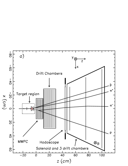
Figure 2: a) A schematic plan view of the detectors, magnet, and target. The solenoid field, shown in the positive y-direction, could be reversed to reduce systematic uncertainties. Tracks from a typical event are superimposed. b) An expanded view of the target region shows the beam-defining scintillators and the veto scintillators used to select events in which only neutral particles exit the target. The hodoscope planes completed the trigger by requiring charged particles downstream of the decay region.

The tracking detectors consisted of two detector stacks. The first was 10 planes of multi-wire proportional chambers with planes alternately oriented at $\pm 45^{\circ}$ relative to the horizontal (the U and V directions). These had a pitch of 1.27 mm and a separation of 1 cm between planes. The second stack was 13 planes of drift chambers oriented vertically and horizontally (the X and Y directions) with an average separation between planes of 1.35 cm. The 4 cm drift cells were read out by a pair of sense wires separated by .42 mm, which resolved the usual left-right ambiguity. A set of three similar but larger drift chambers was located inside the solenoid magnet to determine the direction of deflection of tracks by the 1 kG magnetic field.

Since the beam passed through all these chambers, it was necessary to desensitize the center of each chamber. This was done by electro-plating additional metal onto a 3 to 10 mm length of the relevant sense wires to thicken them at the position at which the beam would pass, preventing gas amplification.

Four planes of microstrips with 100 $\mu$m pitch were located upstream of the target. These provided tracking of the individual incident $\bar{p}$ for a fraction of the events. Four planes provided no redundancy so a beam track could be reconstructed only for events in which exactly one cluster was found on each plane. This applied for only about 45% of events because of beam pile-up and detector-aging in the high intensity beam. For other events the average beam track was used.

The target was enclosed within a 4.2 cm diameter vacuum vessel. Scintillation counters were used to form a trigger which exploited the charged-neutral-charged signature of $\bar{p}p\rightarrow\bar{\Lambda}\Lambda\rightarrow\bar{p}\pi^{+}p\pi^{-}$ events by selecting events in which a $\bar{p}$ entered the target vessel, no charged particles left the target region and at least one charged particle exited the tracking chambers. Figure 2b shows the scintillators used to require an incident $\bar{p}$ and to veto events in which charged particles exit the target area. Figure 2a shows the two scintillator hodoscope planes which indicated a charged decay product.

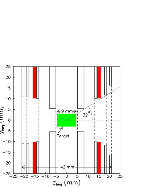
Figure 3: (Color online) Schematic cross-sectional view through the cryostat system (four concentric vertical cylinders) holding the frozen spin target (a horizontal cylinder). Coordinates are indicated relative to the center of the target. The antiproton beam entered through the four thin windows on the left and interacted in the frozen butanol target. Hyperons escaped with relatively little interaction through the large exit windows shown on the right. Dashed lines represent 20 $\mu$m titanium windows while dash-dot lines represent 40 $\mu$m aluminum windows. Coils which provide the holding field are shown shaded. The trigger selected only those events in which the hyperons survived long enough to escape the cryostat and pass the veto detectors before decaying.

The most significant change in the apparatus from previous versions of PS185 was the change from a polyethylene active target to a transversely polarized frozen spin targettarget_thesis . As described above, it has been shown Kent_Brian that this greatly expands the accessible spin information. The target itself was a solid 9 mm long, 6 mm diameter cylinder of frozen Butanol (C₄H₉OH) doped with TEMPO (C₉H₁₈NO)target_material . The axis of the cylinder lay along the beam direction. Figure 3 shows the nested cryostats and the windows which allowed the beam to enter and the $\bar{\Lambda}\Lambda$ to exit. An extremely compact design was achieved to hold the target at 60 mK within a room-temperature outer vacuum vessel of only 2.1 cm radius. Such a compact design was critical to the success of the experiment as it allowed a significant fraction of the $\bar{p}p\rightarrow\bar{\Lambda}\Lambda\rightarrow\bar{p}\pi^{+}p\pi^{-}$ events of interest to be selected by their neutral intermediate state. With a large target vessel the hyperons would have decayed internally and the trigger information would have been lost.

The target was polarized roughly every 22 hours by surrounding it by a superconducting solenoid, with a field of up to 5 T, and pumping with microwaves to achieve dynamic nuclear polarization. Initial polarizations up to 75.3% were achieved. In frozen spin mode, with a holding field supplied by an internal solenoid, polarization lifetime was roughly 100 hours with beam on target. The average polarization over the run was about 62%. The polarization direction was vertical (transverse to the beam) and could be chosen to be positive or negative to reduce systematic errors.

The beam rate on target was approimately $6\times 10^{5}$ antiprotons per second. The integrated beam on target for this measurment was $1.6\times 10^{11}$ antiprotons. Scaling by the data acquisition live time of 79.2% yields an effective integrated intensity of $1.27\times 10^{11}$ antiprotons.

V Data Analysis and Cross Section Results

V.1 Event Reconstruction and Kinematic Fitting

The events of interest, $\bar{p}p\rightarrow\bar{\Lambda}\Lambda\rightarrow\bar{p}\pi^{+}p\pi^{-}$, are characterized by their two-’Vee’ structure resulting from the decay of the neutral hyperons. The first goal of the analysis is to extract the small number of candidates for this event topology from the very large number of events (largely $\bar{n}n$ followed by $\bar{n}$ annihilation) which satisfy the charged-neutral-charged trigger condition. Less than 0.1% of the recorded events were ultimately found to be consistent with the $\bar{p}p\rightarrow\bar{\Lambda}\Lambda\rightarrow\bar{p}\pi^{+}p\pi^{-}$ hypothesis. The next goal is to determine which candidate events match the constraints enforced by energy and momentum conservation on real $\bar{p}p\rightarrow\bar{\Lambda}\Lambda\rightarrow\bar{p}\pi^{+}p\pi^{-}$ events. This is done by kinematic fitting of the event topologies in the tracking chambers, which are in a region free of magnetic field. This fit also provides the best estimate of the production and decay angles of interest and of their correlations. Additionally, information from the three drift chambers within the solenoidal magnetic field is used to determine the sign of the charged particles. If at least one particle’s sign can be clearly determined, then the $\Lambda$-$\bar{\Lambda}$ ambiguity can be resolved and the event can be used in determining spin correlations.

When possible, microstrip information was used in the kinematic fit to define the position and direction of the incoming $\bar{p}$. When this was not possible, average beam position and direction were used. Because of the very small emittance of LEAR’s adiabatically cooled beam, this was sufficiently precise.

Drift chamber wire positions and time-to-distance calibrations were determined empirically from straight track data. This allowed drift chamber hit positions to be accurately determined, typically with better than 200 $\mu$m resolution.

For candidate $\bar{p}p\rightarrow\bar{\Lambda}\Lambda\rightarrow\bar{p}\pi^{+}p\pi^{-}$ events, hit positions were determined from MWPC wire positions and from drift chamber wire position and time. A significant walk correction was made for drift chamber hits based upon time-above-threshold. Hits from all planes sharing a common readout direction (X,Y,U, or V) were then searched for 2-D track projections (X-Z, Y-Z, U-Z, or V-Z). Drift chamber hit positions on a 2-D track candidate were iteratively improved by correcting drift-time to position conversion to reflect the apparent slope of the track. To allow for crossing tracks, a hit could be included in more than one 2-D track. A maximum track angle of 60^∘ was allowed in each projection since tracking was inaccurate beyond that range. Losses due to that cut were accounted for as acceptance losses as discussed in the Sec. V.4.

Combinations of three or more of these 2-D tracks were then considered as candidate 3-D tracks. The 45^∘ rotation of the MWPC projections relative to the drift chamber projections helped eliminate spurious combinations. Confidence-level cuts based on $\chi^{2}$ were used to determine whether sets of 2-D projections were consistent with a 3-D track. Tracks constructed from just two 2-D projections were considered only if neither projection could be used to form a 3-D track having more projections.

Candidate Vee’s were formed from pairs of 3-D tracks having a distance-of-closest-approach consistent with zero. These Vee’s were rejected if they were not consistent with in-flight decay of a $\Lambda$ in the momentum range (471-1161 MeV/c) expected for $\bar{p}p\rightarrow\bar{\Lambda}\Lambda\rightarrow\bar{p}\pi^{+}p\pi^{-}$. A single 3-D track was allowed to be included in more than one Vee to avoid losing a real Vee by having a track mis-assigned to a false Vee.

Pairs of Vee candidates (which did not share any 3-D tracks) were then considered as candidates for kinematic fitting. The pair was first tested for rough consistency with the kinematic hypothesis. (e.g. Transverse components of momentum, calculated independently from the topology of each Vee, should be opposite and equal, within errors.)

For all tracking cuts, simulated events (discussed in Sec. V.2) were used as a guide in setting confidence-level cuts to avoid cutting good events. The simulation included effects due to finite resolution and multiple-scattering.

Kinematic fitting was based upon the fact that the ideal topology of an event (neglecting finite resolution, multiple-scattering, and interactions) can be completely predicted in terms of 14 parameters:

• 3 components of beam momentum

• 3 coordinates of production vertex

• 2 decay lengths

• 2 production angles ($\Theta_{c.m.}$ and $\Phi_{c.m.}$)

• 4 decay angles ($\theta_{\Lambda}$, $\phi_{\Lambda}$, $\theta_{\bar{\Lambda}}$, $\phi_{\bar{\Lambda}}$ ).

The production and decay angles are of greatest interest since they hold the information on the spin dynamics. By varying these 14 parameters it should be possible to find a hypothesis which is consistent with the hits on the observed Vee-pair, within errors. If satisfactory consistency cannot be achieved then the pair can be rejected as not originating from $\bar{p}p\rightarrow\bar{\Lambda}\Lambda\rightarrow\bar{p}\pi^{+}p\pi^{-}$. If an acceptable fit can be found, then it gives the best estimate of the 14 parameters.

When evaluating consistency of a hypothesized set of parameters not only the measured track hits were used but also a data point was included to represent, with appropriate errors, the knowledge of the beam energy and the beam direction for that event. Individual hits (as opposed to tracks) were treated as measurements in evaluating the goodness of fit. The errors on the measurements were not treated as being independent, however. Evaluation of goodness of fit took into account the fact that the errors in hit positions on any given track were correlated because of multiple-scattering. This correlation was increased by the fact that the scattering did not always happen uniformly along a track but could be greatly increased at points where the particle hit a wire of the tracking chambers. Simulated events were used to study the covariance introduced by multiple-scattering and to ensure that the fitting procedure properly accounted for it.

A generalization Kent_thesis of the Levenberg-MarquardtNumerical_recipes method was used to adjust the 14 parameters to minimize a likelihood statistic (analogous to $\chi^{2}$) which accounted for covariance due to multiple-scattering. The estimated errors on parameters were assigned based on the covariance matrix from the fit. As an example of the accuracy of event-reconstruction, the azimuthal production angle $\Phi_{c.m.}$was typically determined with an r.m.s. error of less than $0.4^{\circ}$ (except when it diverged near the poles at $\sin(\Theta_{c.m.})=0$). Also $\cos(\Theta_{c.m.})$ had a mean r.m.s. error of roughly 0.04 for the worst-case events ($\Theta_{c.m.}\approx 90^{\circ}$) falling roughly linearly to less than 0.004 for $0^{\circ}$ and $180^{\circ}$ scattering.

The fit was heavily over-constrained by the measured topology of the event, along with the 12 constraints due to 4-momentum conservation at all three vertices. A rough measure of fit-quality, ${\cal Q}$, was calculated by treating the likelihood statistic as if it were $\chi^{2}$-distributed and calculating the confidence level. A flat distribution over $0\leq{\cal Q}\leq 1$ would be expected from a true $\chi^{2}$ statistic. The actual fit-quality distribution has a large peak below ${\cal Q}=.008$ resulting from unrelated background events (such as anti-neutron annihilation) which produce large numbers of tracks. This very sharp peak was cut early in the analysis and will not be included in the discussion of fit-quality which follows. The remaining Q distribution is shown in Figure 4. The peak at high fit-quality ($0.9\leq{\cal Q}\leq 1.0$) is understood as resulting from events in which no track was substantially deflected by hitting a chamber wire. Conversely, the peak a low Q results largely from events in which one or more track suffered significant deflection. As shown in Figure 4, Monte Carlo simulation correctly predicted the general shape of the observed distribution, including the skew towards high Q and the peaks at large and small ${\cal Q}$. The small residual differences are believed to result from imperfect modeling of the multiple scattering and matter distribution.

Figure 4: Distribution of fit-quality, ${\cal Q}$, found by treating liklihood as if it were distributed with a $\chi^{2}$ statistic. Shown dashed is Monte Carlo prediction, normalized to the data over the interval $.1\leq{\cal Q}\leq 1$.

Events with ${\cal Q}<0.1$ were rejected. This cut not only cleanly rejected the spike of background events at very low Q, it also rejected a significant fraction of the events from quasi-free $\bar{\Lambda}\Lambda$ production on a bound proton in a carbon, oxygen, or nitrogen nucleus in the target. The efficiency of rejection of such events was tested by fitting the $\bar{p}p\rightarrow\bar{\Lambda}\Lambda\rightarrow\bar{p}\pi^{+}p\pi^{-}$ hypothesis to a dataset which was collected using a pure carbon target. These events showed a peak at low ${\cal Q}$, with about half the events being eliminated when events with ${\cal Q}<0.1$ were cut. The remaining tail extended across the ${\cal Q}$ distribution. Scaling that data to the number of non-Hydrogen nuclei in the doped Butanol target, the quasifree contamination can be estimated as 1.7$\pm$0.1% of the final $\bar{\Lambda}\Lambda$ data set. Since the protons involved are unpolarized, this is expected to appear mostly as a dilution of the extracted spin observables. This effect has been included in estimates of the systematic errors.

The cut was expected to reject approximately 9% of good $\bar{p}p\rightarrow\bar{\Lambda}\Lambda\rightarrow\bar{p}\pi^{+}p\pi^{-}$ events and so would be expected to not significantly bias spin correlations unless there was a strong angular variation in the losses. Monte Carlo simulated distributions for azimuthal production angle and individual decay angles matched those of the actual accepted angular distributions, without indication of angular variation of the losses. Furthermore, analysis of Monte Carlo simulated data with the same analysis cuts showed the reconstructed spin-correlation and spin scattering matrix parameters to be in agreement, within expected statistical errors, with those used to generate the Monte Carlo events.

Kinematic fitting in the field-free region cannot distinguish the $\Lambda$ from the $\bar{\Lambda}$. Tracks were extended into the solenoid and the three drift chambers there were searched for triplets of hits which could be used to assign a charge to at least one of the tracks. The hits were compared to predictions based upon the reconstructed momentum and angle of the track and both possible charges. Expected covariance of the hits, which was large because of multiple-scattering in the coils of the solenoid, was taken into account. Any track which was well fit by one charge hypothesis acted as a ’vote’ for which Vee was the $\Lambda$. In principle a single vote was sufficient to resolve the ambiguity and properly identify all four tracks. Events with multiple votes occasionally had two tracks which voted differently on which Vee should be identified as the $\Lambda$. Additionally, 8% of the events were unusable because they had no vote or had conflicting votes.

A naïve estimate of the error rate of these individual votes can be achieved by assuming the error rate is a constant, uncorrelated with the number of votes. The rate of inconsistency between the votes in two-vote events would then imply a 3.1% error rate on individual tracks. Assuming that the same error rate applies for those events which have only a single vote leads to the estimate that in total the $\Lambda-\bar{\Lambda}$ identification was interchanged in 1.1% of the reconstructed events.

More careful evaluation however shows that this naïve estimate under-predicts the actual rate of inconsistency for multiple-vote events, indicating a correlation between number of votes and error rate. Without adjustable parameters, the Monte Carlo simulation described in the next section makes an excellent prediction of both the observed distribution of number of votes per event and the rate of inconsistent votes as a function of the number of votes. This gives some confidence in the Monte Carlo prediction that the actual fraction of events in which the $\Lambda-\bar{\Lambda}$ identification was interchanged is only 0.7% with no marked dependence on $\Theta_{c.m.}$. The smaller value results from the Monte Carlo’s prediction of a lower error rate for single-vote events than for two-vote events.

Combining these two estimates, a ($0.9\pm 0.2$)% misidentification rate was assumed when correcting for contamination as explained in Sec. V.4. The estimated error of $\pm 0.2$% was included in the systematic error analysis. This contamination was negligible in all but the two most back-angle bins.

A total of 30818 events were successfully kinematically reconstructed as $\bar{\Lambda}\Lambda$ events with the $\Lambda$-$\bar{\Lambda}$ ambiguity resolved.

V.2 Monte Carlo Simulation

An understanding of the angular dependence of acceptance is critical to successful extraction of spin scattering information from angular distributions. The acceptance function used to extract spin observables was evaluated using a simulation designed to incorporate empirical detector response along with predicted particle interactions. The Monte Carlo simulation was also used in tuning algorithms and setting cuts to optimize tracking, Vee-finding, and fitting. Simulated events were also used to study systematic errors.

The GEANT-based GEANT simulation included multiple-scattering, $\delta$-ray production, and hadronic interactions. The latter was especially important for the final-state $\bar{p}$, which has a large annihilation cross-section. The description of the mass distribution included the target, cryostat, scintillators, chamber foils, gas, and wires.

The position and response of detectors were determined empirically when possible and used as input for simulation. Positions of trigger scintillators were determined by tracking through the micro-strip detectors using data from dedicated calibration runs taken with a thick scatterer upstream of the microstrips. These data were also used to determine tracking chamber positions and to measure their efficiencies as a function of track slope and position.

Simulation of the wire chambers included observed decrease in chamber efficiencies near the sense wires, the observed effective size of the ’dead spot’ built into the center of each plane, and the observed decrease in efficiency on the neighboring drift chamber sense wire due to field distortion at the ’dead spot’.

The effect of the trigger scintillators was an important component of the simulation. Use of trigger scintillators was essential to select out the rare events of interest. The cryogenic target however made it impossible to place the scintillators as close to the production point as had been done in all previous versions of the PS185 experiment. Therefore a large fraction of all $\bar{p}p\rightarrow\bar{\Lambda}\Lambda\rightarrow\bar{p}\pi^{+}p\pi^{-}$ events were lost because at least one hyperon decay occurred upstream of the veto scintillators.

Figure 5 shows a comparison between simulated and measured distributions, as an example of a test of the simulation. The z component of vertex position of $\Lambda$ decay is shown. The distribution is seen to be well predicted by simulation, including the sharp rise due to the position of the veto scintillators. The target, as shown in Fig. 3b, is located upstream of this position but the veto scintillators prevent triggers for events in which the decay occurs further upstream.

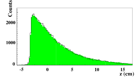
Figure 5: (Color online) Comparison of the hyperon decay vertex $z$-coordinate distributions between data (solid line) and simulated data set (shaded).

V.3 Differential Cross Section

The $\Phi_{c.m.}$-averaged differential cross section for $\bar{\Lambda}\Lambda$ production at $p_{\bar{p}}=1.637$ GeV/c can be found from the spin-matrix parameters {a,b,c,d,e,g}, determined as described in the following sections, as

$$<\,\begin{array}[]{c}d\sigma\\ \hline\cr d\Omega_{\Lambda}\end{array}\,>\ \equiv\ \frac{1}{2\pi}\,\begin{array}[]{c}d\sigma\\ \hline\cr d\cos\Theta_{c.m.}\end{array}\,=I_{0}$$

$$= \frac{1}{2}\{a^{2}+b^{2}+c^{2}+d^{2}+e^{2}+g^{2}\}.$$

The differential cross section so found is shown as dark points in Fig. 6. The cross section is essentially identical to that found by counting $\bar{\Lambda}\Lambda$ events within each $\cos(\Theta_{c.m.})$ bin and correcting for mean acceptance over the angular distributions found below.

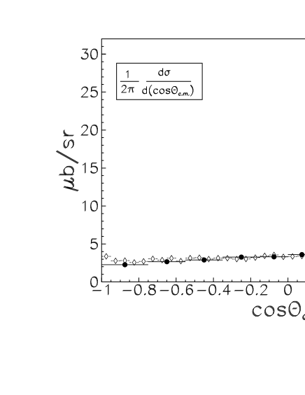
Figure 6: Results for the $\phi$-averaged differential cross section (solid). The previous measurement Horsti at $1.642\,\mbox{GeV}/\mbox{c}$, scaled by a factor of 1.26 to match present integrated cross section, is superimposed (open diamonds).

The unequal bin widths seen in Fig. 6 were chosen to give roughly equal statistics of observed $\bar{\Lambda}\Lambda$ events in each of sixteen $\cos(\Theta_{c.m.})$ bins. This allowed a stable fit of the eleven spin-matrix parameters to be performed in each bin. Uniform binning would have sacrificed forward-angle $\cos(\Theta_{c.m.})$ resolution or resulted in low-statistics fits at back angles leading to instability and large errors. The cross section is discussed here, in advance of the explanation of the fitting procedure, to motivate this choice of $\cos(\Theta_{c.m.})$ bins, which applies to all subsequent discussion of the matrix parameters.

The open points in Fig. 6 show a renormalized version of a previously published result Horsti from an earlier version of the PS185 experiment using unpolarized polyethylene target cells surrounded by scintillator. That measurements were made at $p_{\bar{p}}=1.642$ GeV/c which is very nearly the same beam momentum as the present data, $p_{\bar{p}}=1.637$ GeV/c. For the purpose of comparison of shapes, the older result has been scaled up by a factor of 1.26 to match the integrated cross section of $81.1\pm 0.5^{+5.8}_{-7.5}\,\,\mu b$ measured in the present experiment (where the first error is statistical and the second is systematic). The systematic errors assigned to the present measurement are larger than on earlier ones because the cryogenic polarized target introduced larger uncertainties in target thickness, target position relative to trigger counters, and hadronic interactions. As described in Sec. V.5, these systematic errors have been realistically estimated so an explanation is required for the apparent discrepancy between the present and previous determinations of total cross section. The normalization discrepancy in early PS185 results has already been described in an earlier publication threshold . Hadronic interactions and multiple scattering were not included in the custom-written Monte Carlo simulation code used to determine acceptance corrections in early analyses of PS185 data old_PS185 ; Horsti . Versions of a GEANT-based simulation have been used in calculating acceptances for more recent results threshold ; recent_PS185 . Inclusion of hadronic interactions and multiple scattering increased the estimated yield by 8-12%. With a $10\pm 2$% adjustment in normalization, the older result gives $\sigma=70.4\pm 0.4\pm 2.2\,\mu b$ which roughly agrees with the present result within errors. The spin-correlations are insensitive to any systematic error on overall normalization.

Comparison of the two data sets in Fig. 6 shows some difference in shape of the distribution at forward angle. The present analysis took into account correlated errors due to track deflections caused by multiple-scattering. This allowed events to be reconstructed which might otherwise have been lost. The older analysis did not allow for multiple-scattering in event reconstruction. The lost events would not have been compensated by acceptance corrections since multiple-scattering was not included in the Monte Carlo simulation. Furthermore, estimates of expected losses, found by disabling the multiple-scattering correlation in fitting in the present analysis, indicate that the effect is greatest at forward and back angles, where hyperon momenta are low. The sharper peak at forward angles seen in the present data is therefore believed to be accurate while the older data is slightly distorted by multiple-scattering losses.

V.4 Fitting Spin-scattering Matrix Parameters

For each bin in $\Theta_{c.m.}$, Eq. (11) represents the distribution of events across a 5-dimensional space of angles ($\Phi_{c.m.},\ \cos(\theta_{\bar{\Lambda}}),\ \phi_{\bar{\Lambda}},\ \cos(\theta_{\Lambda}),\ \phi_{\Lambda}$) which will be represented by a 5-dimensional vector, $\vec{v}$ for notational convenience. With only roughly 2000 events in each $\Theta_{c.m.}$ bin, performing a simple $\chi^{2}$-fit by subdividing each of the five coordinates into bins is excluded. An unbinned maximum-likelihood fitting technique was employed. This is often called simply ’maximum-likelihood fitting’ a name which fails to distinguish from other fit methods such as $\chi^{2}$ minimization, which also correspond to a maximum likelihood.

Unbinned fitting is a limiting case of fitting with Poisson statistics. If the data were binned into $K$ bins with $n_{k}$ being the number of events in bin $k$, then the likelihood of the observed data set would be

$${\mathcal{L}}=\prod_{k=1}^{K}e^{-\phi(\vec{v}_{k},\vec{a})\Delta\vec{v}_{k}}\{\frac{(\phi(\vec{v}_{k},\vec{a})\Delta\vec{v}_{k})^{n_{k}}}{n_{k}!}\}$$

where $\phi(\vec{v}_{k},\vec{a})$ is the probability density function which depends on the eleven real parameters of the spin-scattering matrix, here represented as the 11-dimensional vector $\vec{a}$. The volume of the k’th 5-dimensional bin is $\Delta\vec{v}_{k}$. If the number of bins, $K$, now becomes large compared to the number of events, $N$, then $n_{k}$ will be zero for most bins and will be unity for $N$ bins. In this limit the likelihood becomes

$${\mathcal{L}}=\prod_{k=1}^{K}e^{-\phi(\vec{v}_{k},\vec{a})\Delta\vec{v}_{k}}\prod_{j=1}^{N}\phi(\vec{v}_{j},\vec{a})\Delta\vec{v}_{j}$$

where the second product runs over only the occupied bins. Neglecting background contamination, $\phi$ is the intensity distribution, described by Eq. (11), scaled by the integrated luminosity of the experiment, the solid angle corresponding to the $\Theta_{c.m.}$-bin considered, and the average acceptance probability for coordinates $\vec{v}_{k}$, $\vec{v}_{k}$.

Taking the log of ${\mathcal{L}}$ introduces a sum of $\ln(\Delta\vec{v}_{j})$ terms which would diverge in the limit of infinitesimal bin size. Since these terms are independent of $\vec{a}$, discarding them does not change the value of $\vec{a}$ which maximizes the likelihood. Let ${\cal M}^{\prime}$ represent $-2\ln({\cal L})$ with these terms discarded. Then in the limit of infinitesimal bin size,

$${\cal M}^{\prime}=2\int\phi(\vec{v},\vec{a})\ d\vec{v}-2\sum_{j=1}^{N}\ln(\phi(\vec{v}_{j},\vec{a}))$$

Maximization of the likelihood for a data set {$\vec{v}_{1}$ … $\vec{v}_{N}$} can be accomplished by finding the parameters, $\vec{a}$ which minimize ${\cal M}^{\prime}$. Writing $\phi(\vec{v},\vec{a})$ as $\mu(\vec{v},\vec{a})A(\vec{v})$ where A is the acceptance and $\mu$ is the remainder of the probability density function (which, neglecting background contamination, would be $I_{final}(\Theta_{c.m.},\Phi_{c.m.},\hat{k}^{\bar{p}},\hat{k}^{p})$ scaled by the integrated luminosity and the solid angle),

$${\cal M}^{\prime}=2\int\mu(\vec{v},\vec{a})A(\vec{v})\ d\vec{v} - 2\sum_{j=1}^{N}\ln(\mu(\vec{v}_{j},\vec{a}))$$

$$- 2\sum_{j=1}^{N}\ln(A(\vec{v}_{j}))$$

The last term, which is independent of $\vec{a}$, can be discarded without affecting the position of the minimum. This gives the final function to be minimized, which will be called ${\cal M}$.

The first term of ${\cal M}$, which incorporates the acceptance function, could in principle be evaluated by Monte-Carlo integration (with each simulated event being processed by the analysis routines to see whether it would be successfully reconstructed). However, minimization of ${\cal M}$ would then require prohibitive re-evaluation of this term for each new set of parameters $\vec{a}$ being tested. Fortunately the structure of $I_{final}$ in Eq. (11) permits a great simplification. Each of the twenty terms of Eq. (11) can be written as a product with an $\vec{a}$-dependent dynamic term (containing the Q’s and $I_{0}$) multiplying a purely geometric term, $G_{i}(\vec{v})$, which depends on $\vec{v}$ but not on the parameters $\vec{a}$. So $\mu$ can be written as

$$\mu(\vec{v},\vec{a})=\sum_{i=1}^{20}D_{i}(\vec{a})G_{i}(\vec{v})$$

allowing the first term of ${\cal M}$ to be simplified since

$$\int\mu(\vec{v},\vec{a})A(\vec{v})\ d\vec{v} = \sum_{i=1}^{20}D_{i}(\vec{a})\int G_{i}(\vec{v})A(\vec{v})\ d\vec{v}$$

$$= \sum_{i=1}^{20}D_{i}(\vec{a})W_{i}$$

where the weights $W_{i}$ are the moments of the acceptance which are independent of $\vec{a}$ and so need to be evaluated only once by Monte-Carlo integration. To perform this integration the simulation was used to generate events uniformly distributed in $\vec{v}$-space without weighting to match the observed spin-correlations. The fitting procedure is then to search for $\vec{a}$ which minimizes

$${\cal M}=2\sum_{i=1}^{20}W_{i}D_{i}(\vec{a})-2\sum_{j=1}^{N}\ln(\mu(\vec{v}_{j},\vec{a}))$$

As explained above, an estimated $(0.9\pm 0.2)$% rate of mis-identification of $\Lambda$ and $\bar{\Lambda}$ causes contamination of $\Theta_{c.m.}$ bins with data from the supplementary angle. Because the differential cross section is strongly forward-peaked, this is a negligible effect except for the two most back-angle bins. The predicted mis-identification rate at forward angles leads to an 8% contamination of the most back-angle bin. To allow for this, the $\mu(\vec{v})$ used in back angle bins was not simply $I_{final}(\vec{v},\vec{a})$ scaled by the integrated luminosity and solid angle. Rather, $I_{final}(\vec{v},\vec{a})$ was replaced by an appropriately weighted linear combination of $I_{final}(\vec{v},\vec{a})$ and the background term $I_{final}(\vec{v}_{reversed},\vec{a}_{forward})$ where $\vec{v}_{reversed}$ is the corresponding point in $\vec{v}$-space reached by reversing $\Lambda$ and $\bar{\Lambda}$ identification and $\vec{a}_{forward}$ is the set of parameters which applies for the forward-angle bin. Fitting of forward-angle bins was carried out first to allow this contamination to be correctly modeled when fitting the back-angle bins.

Minimization in the 11-dimensional $\vec{a}$-space was accomplished by the Polak-Ribière conjugate gradient method Numerical_recipes . To guard against false minima, each minimization was carried out multiple times with different randomly-chosen starting points. For most $\cos(\Theta_{c.m.})$ bins a common minimum was found in every search. In the worst case the fit converged on false minimum less than 65% of the time. Additionally, Monte Carlo simulated data sets were generated with similar statistics and spin-correlations to the actual data. Fitting these simulated data sets demonstrated the robustness of the technique for converging on the proper minimum and allowed determination of a scale of confidence level for numerical values of ${\cal M}$. Unlike $\chi^{2}$, ${\cal M}$ has no a priori expected value for good fits because it is arbitrarily offset from the true log-likelihood. There was no indication that ${\cal M}$ values obtained for the real data were systematically higher than what was expected for a good fit, based on values obtained for corresponding simulated data sets.

Use of the curvature matrix, based on the assumption of parabolic behavior of ${\cal M}$ near the minimum, was found to give inaccurate estimates of the errors on the $\vec{a}$ parameters. Errors were instead determined by using a ’brute-force’ search of the space around the minimum to find the maximum possible change in each parameter (in conjunction with changes in all other parameters) consistent with an increase of less than one in the value of ${\cal M}$. Since ${\cal M}$ differs from $-2\ln({\cal L})$ only by a constant offset, a given change in ${\cal M}$ has the same interpretation as the equivalent change in $-2\ln({\cal L})$. These maximum-acceptable (positive- and negative-) changes in each parameter will be referred to as the ’$1\sigma$’ errors since they cover the confidence interval which would be covered by $1\sigma$ in the case of Gaussian errors. Similarly, a ’$2\sigma$’ error bound on each parameter was found by finding the maximum possible (positive or negative) change in each parameter for which ${\cal M}$ would exceed its minimum value by less than $4$.

Once the best-fit parameters $\vec{a}$ have been found, $I_{0}$ and all the Q’s can be determined (even those Q’s not directly measurable in an experiment with unpolarized beam and a transverse target polarization). But, since the errors on the parameters are highly correlated, the error on each spin-correlation cannot be determined by simple lowest-order error propagation. Even if the correlation matrix were determined, error propagation would be unreliable. A far superior estimate of the error on each spin-correlation comes from the same ’brute-force’ search for $\Delta{\cal M}=1$ and $\Delta{\cal M}=4$ regions. At each point, all quantities of interest, such as spin-correlations, were calculated. The maximum positive and negative excursions of each such quantity from its best-fit value, consistent with $\Delta{\cal M}<1$ and $\Delta{\cal M}<4$, were taken to be the ’$1\sigma$’ and ’$2\sigma$’ errors, respectively, on that calculated quantity.

V.5 Systematic Errors

Overall normalization errors would not affect measured spin-correlations but would directly change $I_{0}$ and equivalently the $\Phi_{c.m.}$-averaged differential cross section presented in Fig. 6. Since the focus of the experiment was on spin-correlations, overall normalization was not controlled as carefully as other aspects of the experiment. The length of the cylindrical frozen Butanol target was measured to be $9.0\pm 0.5$ mm. An upper limit on the misalignment of the target axis relative to the beam was $20^{\circ}$ which could increase effective target thickness by up to 6%. The uncertainty in effective position of veto scintillators relative to the target was estimated at 1 mm which was found, through Monte Carlo simulation, to cause less than 4% uncertainty in normalization. Statistical error in the estimate of quasi-free contamination introduced a negligible systematic error. The overall fractional systematic uncertainty, estimated by adding these contributions in quadrature, is ${+7.1\%}/{-9.3\%}$. This gives the systematic error, quoted above, on the total cross section, $\sigma=81.1\pm 0.5^{+5.8}_{-7.5}\mu b$. This same fractional systematic error applies to the bins of $<\frac{d\sigma}{d\Omega}>$ in Fig. 6. While the normalization error cancels in spin-observables, all spin-matrix parameters would scale by the square-root of any overall normalization factor. Since this is a common factor on all terms, it is not included in the error band assigned to each of these parameters. It should be remembered that an overall normalization error of ${+3.5\%}/{-4.8\%}$ applies to the spin-matrix parameters.

The reconstructed angles for each event, $\vec{v}_{k}=(\Phi_{c.m.},\ \cos(\theta_{\bar{\Lambda}}),\ \phi_{\bar{\Lambda}},\ \cos(\theta_{\Lambda}),\ \phi_{\Lambda}$), are not known exactly but are extracted with known errors and correlations. The method of unbinned maximum-likelihood fitting treats each event as a precise point in the 5-dimensional $\vec{v}$-space and does not incorporate a method of allowing for the finite errors on these points. Neglecting these finite errors introduces a source of systematic error in addition to the statistical error discussed above. The method of estimating these systematic errors was based on the use of simulated data with errors and event statistics similar to the actual data. These simulated data sets were generated based on spin-correlations chosen to nearly match those found in the data. Simulated events were kinematically fit giving $\vec{v}_{k}$’s with errors similar to the real data. Unbinned maximum-likelihood fits were then used to extract best-fit values of the spin-transfer matrix parameters, which were then used to calculate spin-correlations and all other variables of interest, as described in the next section. The fitting process was then repeated using the ideal $\vec{v}_{k}$’s which had been used by the Monte Carlo to generate the simulated data. The differences between best-fit values of each variable fit to the simulated data and the best-fit values fit to the ideal $\vec{v}_{k}$’s was a measure of the systematic error in that variable because of the finite resolution of the $\vec{v}_{k}$’s. Changes in each variable of interest were calculated independently, rather than using error-propagation to extract the expected effect. Ideal fits were compared to fits using kinematically fit finite-resolution data for ten different simulated data sets. Additionally, since kinematic fitting was quite time-consuming, the statistics of this study were augmented by generating an additional 20 data sets by simply smearing each ideal $\vec{v}_{k}$ by its estimated resolution rather than simulating an event and operating the full analysis chain on it. Estimates of systematic error due to finite resolution were thus found as the r.m.s. shift from the zero-resolution value for each variable of interest in each $\Theta_{c.m.}$ bin. This contribution typically dominated the overall systematic error estimates which are shown with each variable in the next section.

The non-hydrogen nuclei in the target were unpolarized so quasi-free events mis-identified as free $\bar{p}p\rightarrow\bar{\Lambda}\Lambda\rightarrow\bar{p}\pi^{+}p\pi^{-}$ events will exhibit no correlation to target polarization direction. The effect of the small quasi-free contamination can therefore be estimated by introducing an appropriate fraction of isotropically-distributed simulated events in place of some of the events of a simulated data set. The estimated quasi-free contamination (from analysis of carbon-target data) was typically only about 1% but rose to 3% at farthest back-angle. Systematic errors for each variable of interest were again found by determining the r.m.s. shift of that variable caused by the simulated contamination. This small contamination generally caused smaller systematic errors than did the effects of finite resolution.

Several precautions were taken to reduce systematic effects due to target polarization. The direction of target polarization was reversed during data collection to cancel systematic effects due to any up-down asymmetry of the detectors. Average target polarization was measured by Nuclear Magnetic Resonance measurements at the beginning and end of each data-collection period (between target re-polarizations) to improve estimates of its value at intermediate times. Data-collection periods were typically limited to a quarter of the polarization lifetime to keep the polarization high and to improve accuracy of estimated polarization. The probability density function used to weight each measurement in the unbinned fit was not based upon an average polarization but on the best estimate of the polarization at the time that event was recorded.

An additional systematic error results from uncertainty in initial polarization and from possible inhomogeneities in target relaxation. The fractional error in measured target polarization is estimated at ${\Delta P}/{P}=2.3\%$. The average polarization measured at the end of a data-collection period could not determine whether depolarization was non-uniform due to beam heating. However the target was kept cold enough that relaxation time was not strongly temperature-dependent. Inhomogeneity of depolarization is estimated to contribute an uncertainty of at most ${\Delta P}/{P}=3.8\%$ just before repolarization. These errors combined to give a worst-case estimate of ${\Delta P}/{P}=4.5\%$ at the end of the data-collection period.

The maximum systematic error due to polarization was estimated by shifting polarizations by 4.5% and determining the size of the shift of extracted observables of interest. This was found to be a smaller error than that due to resolution or quasifree background. All three effects were added in quadrature bin-by-bin for all variables of interest to obtain the overall systematic error estimate which is plotted as an error band at the bottom of plots of each variable of interest.

VI Spin Correlation Results

Figures 7 and 8 show the best-fit values of the 11 parameters of the spin-scattering matrix fit to the data in bins of $\Theta_{c.m.}$. Parameter ’a’ is chosen to be real (and non-negative) so Im(a) is zero. On each point the dark bar indicates the ’$1\sigma$’ error range while the light bar represents the ’$2\sigma$’ error. Because of the actual shape of the ${\cal M}$-hypersurface, some of the error bars are highly asymmetric and the ’$2\sigma$’ error is often very different from twice the ’$1\sigma$’ error. The black band at the bottom of each plot indicates the estimated systematic error. Overall normalization error is not included in the systematic-error band. These, and other results presented below are available in table formEPAPS .

Figure 7: Fit results for spin matrix parameters a, b, and c. The arbitrary phase is chosen by constraining the parameter $a$ to be real and non-negative. Statistical errors are shown on each data point, with $2\sigma$ error bars superimposed (dashed). The estimated systematic error width is shown at the bottom of each plot (dark-shaded region).

Figure 8: Fit results for spin matrix parameters d, e, and g. Statistical errors are shown on each data point, with $2\sigma$ error bars superimposed (dashed). The estimated systematic error width is shown at the bottom of each plot (dark-shaded region).

Table 2 shows how each of the 19 directly measurable spin-correlations (and $I_{0}$) can be calculated from the parameters $\vec{a}$ for the spin-scattering matrix. While the spin-correlations can be calculated directly from the best-fit values of the parameters, as explained above, their errors cannot be found by propagation of the errors on the parameters. Results for $I_{0}$ (= $<\frac{d\sigma}{d\Omega}>$ ) have already been shown in Fig. 6 above. Results for the polarization $Q[n_{\Lambda}]=Q[n_{\bar{\Lambda}}]$, often denoted $P_{\Lambda}$ and $P_{\bar{\Lambda}}$, are shown in Fig. 9 as filled circles with ’$1\sigma$’ and ’$2\sigma$’ errors indicated. Also shown are results from the previous PS185 measurement Horsti at $p_{\bar{p}}=1.642$ GeV/c which can be seen to be in good agreement. Similarly Fig. 10 shows those 2-spin correlations which can be measured without a polarized target. These correlations of the spins of the final-state $\Lambda$ and $\bar{\Lambda}$ are commonly denoted $C_{mm}$, $C_{ml}$, $C_{nn}$, and $C_{ll}$. Again good agreement is seen with the previous results.

Figure 9: Current results for polarization, $Q[n_{\Lambda}]=Q[n_{\bar{\Lambda}}]$ (filled circles). The previous measurement Horsti at $1.642\,\mbox{GeV}/\mbox{c}$ is superimposed (open squares). Statistical errors are shown on each current data point, with $2\sigma$ error bars superimposed (dashed). The estimated systematic error width is shown at the bottom of each plot (dark-shaded region).

Figure 10: Current results for previously measured spin correlations between $\bar{\Lambda}$ and $\Lambda$ (filled circles). Previous measurements Horsti are superimposed (open squares). Statistical errors are shown on each current data point, with $2\sigma$ error bars superimposed (dashed). The estimated systematic error width is shown at the bottom of each plot (dark-shaded region). The spin correlations shown are a) $Q[m_{\bar{\Lambda}},m_{\Lambda}]$, b) $Q[m_{\bar{\Lambda}},l_{\Lambda}]$, c) $Q[n_{\bar{\Lambda}},n_{\Lambda}]$, and d) $Q[l_{\bar{\Lambda}},l_{\Lambda}]$.

A particular combination of these observables, which has direct physical interpretation, is the singlet fraction (the fraction of $\bar{\Lambda}\Lambda$ pairs which are produced in a spin-singlet state) which can be written as

$$S_{F}=\frac{1}{4}(1-Q[n_{\Lambda},n_{\bar{\Lambda}}]+Q[m_{\Lambda},m_{\bar{\Lambda}}]+Q[l_{\Lambda},l_{\bar{\Lambda}}])$$ (14)

This can be calculated directly from the spin-scattering matrix parameters as

$$S_{F}=\frac{|b-c|^{2}}{4I_{0}}$$ (15)

This is shown in Fig. 11. Again the errors have been assigned by directly determining the limits of change in $S_{F}$ for a maximum acceptable change in log-likelihood. Previous PS185 results Horsti at $p_{\bar{p}}=1.642$ GeV/c are shown for comparison. The earlier results were determined from Eq. (14) using spin-correlations which had been separately extracted from the data. Unphysical negative values could then occur as a result of statistical fluctuations or heightened sensitivity to systematic errors in the linear combination of observables. The present results were extracted using Eq. (15) and so are constrained to be non-negative throughout the range of their error bars. It is interesting to note that the often-accepted empirical rule that $S_{F}=0$ for this reaction is clearly broken at back angles.

Figure 11: Current results for singlet fraction $\text{S}_{F}$ (filled circles). The previous measurement Horsti is superimposed (open squares). Statistical errors are shown on each current data point, with $2\sigma$ error bars superimposed (dashed). The estimated systematic error width is shown at the bottom of each plot (dark-shaded region).

Figure 12 shows results for $Q[n_{p},n_{\Lambda}]$ and $Q[n_{p},n_{\bar{\Lambda}}]$ conventionally denoted as $D_{nn}$ and $K_{nn}$, respectively. These results, which have already been published in Bernd_et_al , are seen to disagree strongly with predictions from both meson-exchange MEX_pred and quark-gluon QG_pred models. While these results have been published, the present paper is the first to document the details of the technique used to extract them. Measurement of these spin-correlations was the main goal of this experiment because two competing classes of models made differing firm predictions for these observables. While both classes of model had enjoyed success in explaining the observations made with unpolarized targets, these results suggest that additional dynamics will have to be included into the models. The wealth of additional spin-dynamics information presented below may help constrain and test refinements made to match the surprising results in these two spin-correlations.

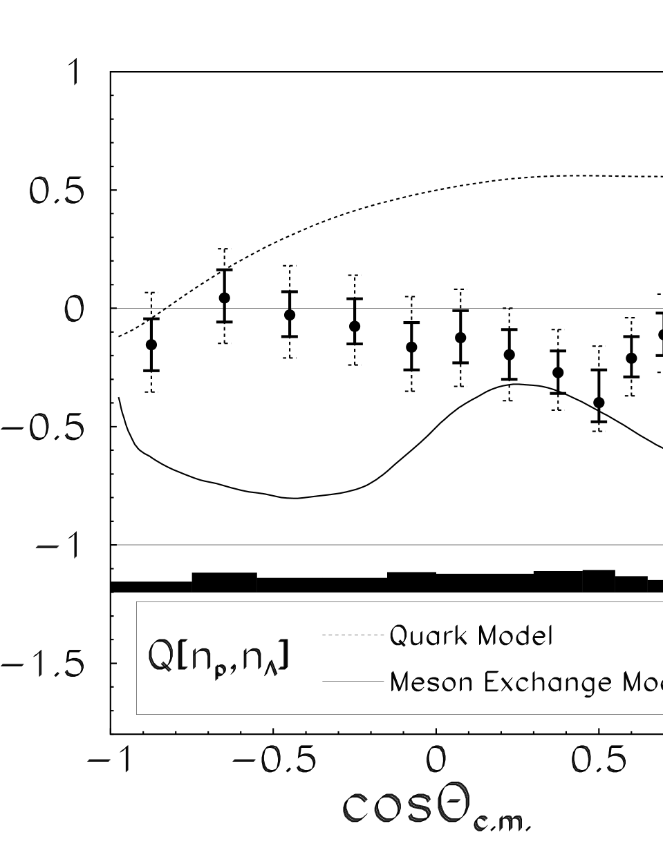
Figure 12: Results for spin transfer observables $Q[n_{p},n_{\Lambda}]$ (often called depolarization, $D_{nn}$) and $Q[n_{p},n_{\bar{\Lambda}}]$ (often called spin-transfer, $K_{nn}$) at $1.637\,\mbox{GeV}/\mbox{c}$, compared to MEX model prediction MEX_pred (solid) and QG model prediction QG_pred (dashed) at $1.642\,\mbox{GeV}/\mbox{c}$. Statistical error bars are shown on each data point, with $2\sigma$ error bars superimposed (dashed). The estimated systematic error width of the measurement is shown at the bottom of each plot (dark shaded region).

The remaining 12 directly measurable spin-correlations are shown in Fig. 13 The first of these, Q[n_p], is the analyzing power, often denoted A_n. The remainder are correlations between initial proton spin and components of one or both final-state spins. Errors are seen to be small enough, even on most 3-spin correlations, to allow structures to be clearly resolved. This underscores the advantage of fitting the spin-scattering matrix parameters. If these directly measurable spin-correlations had been determined by a direct fit of Eq. (11) to the observed distribution, their errors would have been much larger and so meaningful structure would have been impossible to extract in most cases.

Figure 13: Results for the twelve additional spin observables which appear directly in the measured angular distribution. Statistical and systematic error estimates are displayed, as above. The spin observables displayed are a) $Q[n_{p}]$, b) $Q[m_{p},m_{\Lambda}]$, c) $Q[m_{p},l_{\Lambda}]$, d) $Q[m_{p},m_{\bar{\Lambda}}]$, e) $Q[m_{p},l_{\bar{\Lambda}}]$, f) $Q[m_{p},m_{\bar{\Lambda}},n_{\Lambda}]$, g) $Q[m_{p},n_{\bar{\Lambda}},m_{\Lambda}]$, h) $Q[m_{p},n_{\bar{\Lambda}},l_{\Lambda}]$, i) $Q[m_{p},l_{\bar{\Lambda}},n_{\Lambda}]$, j) $Q[n_{p},m_{\bar{\Lambda}},m_{\Lambda}]$, k) $Q[n_{p},m_{\bar{\Lambda}},l_{\Lambda}]$, and l) $Q[n_{p},l_{\bar{\Lambda}},m_{\Lambda}]$

Of the 256 spin-correlations, $Q[j_{\bar{p}},k_{p},\mu_{\bar{\Lambda}},\nu_{\Lambda}]$, defined by Eq. (6), one is trivially unity and 128 are constrained to be zero by parity conservation of the strong interaction. An additional 88 can be neglected because symmetry requires that they are identical to (or the negative of) another one which is being considered. In this sense there are 39 non-trivial spin correlations in addition to $I_{0}$. These cannot be said to be forty independent observables since they can be expressed in terms of just eleven real parameters of the spin-scattering matrix at each $\Theta_{c.m.}$. However there are 40 quantities which would be directly measurable given arbitrary beam and target polarization. Of these, twenty (including $I_{0}$) are directly measurable in the present experiment and have been presented above. However, since the spin-scattering matrix is fully determined, the remaining 20 spin-correlations can equally well be extracted just as the directly measurable ones are in the present analysis. The eight such observables shown in Fig. 14 would be directly measurable (i.e. would appear explicitly in the description of the angular distribution) without a polarized beam if the target were longitudinally polarized. Although the target polarization in the present experiment is purely transverse, these observables are still determined, and in some cases determined quite accurately, in this present measurement. Similarly, Fig. 15 gives the results for spin observables which would be directly measurable only if the antiproton beam were polarized. Again, some of these are quite well determined by the present data set. In rare cases a double-minimum in the log-likelihood function, ${\cal M}$, results in disjoint regions falling within the 1$\sigma$ limit. These are indicated in Fig. 15 by a second disjoint error bar.

Figure 14: Results for eight spin observables which do not appear directly in the measured angular distribution. Direct measurement of an individual one of these observables would require a longitudinally polarized target proton but would not require beam polarization. Statistical and systematic error estimates are displayed, as above. The spin observables displayed are a) $Q[l_{p},m_{\Lambda}]$, b) $Q[l_{p},l_{\Lambda}]$, c) $Q[l_{p},m_{\bar{\Lambda}}]$, d) $Q[l_{p},m_{\bar{\Lambda}},n_{\Lambda}]$, e) $Q[l_{p},n_{\bar{\Lambda}},m_{\Lambda}]$, f) $Q[l_{p},n_{\bar{\Lambda}},l_{\Lambda}]$, g) $Q[l_{p},l_{\bar{\Lambda}}]$, and h) $Q[l_{p},l_{\bar{\Lambda}},n_{\Lambda}]$.

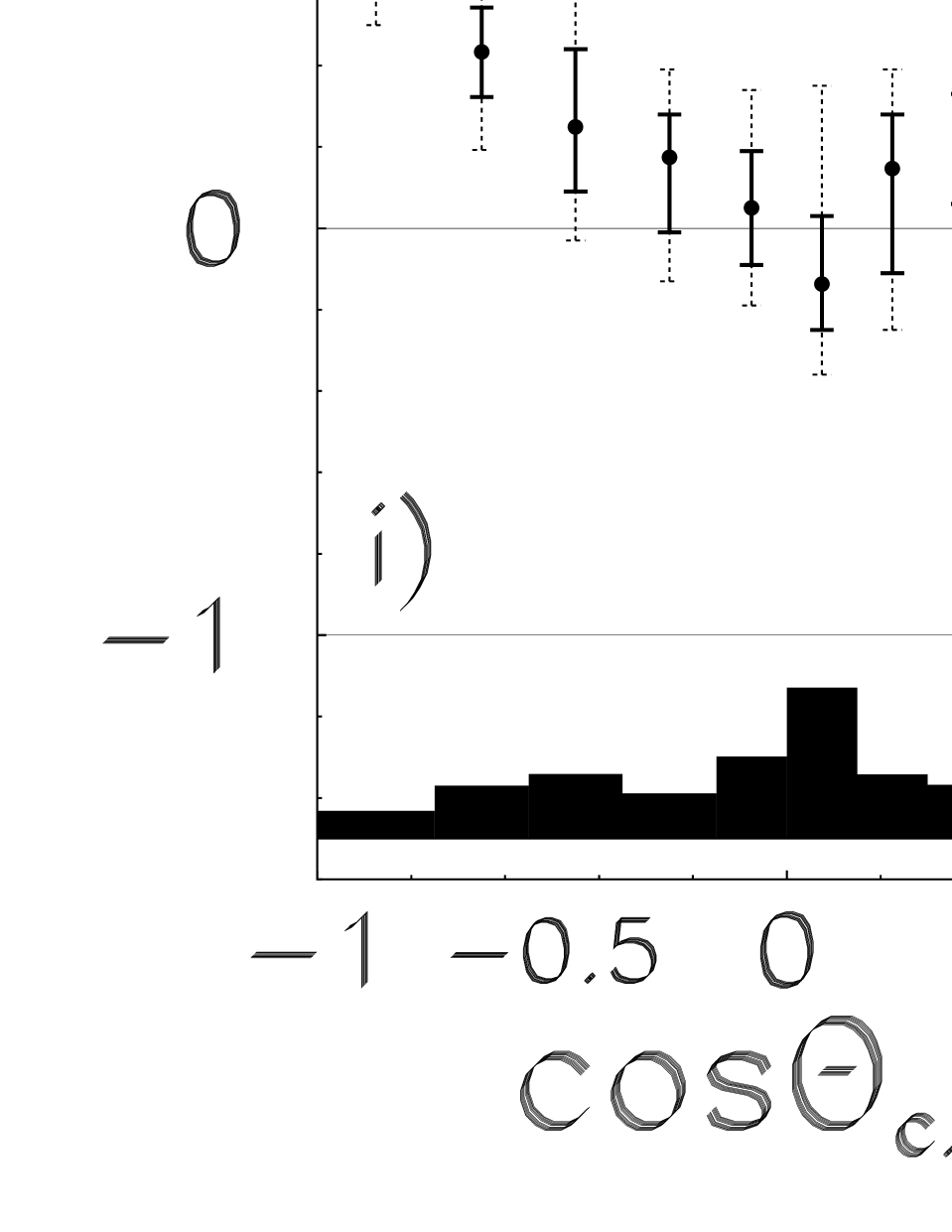
Figure 15: Results for the final twelve spin observables which do not appear directly in the measured angular distribution. Direct measurement of an individual one of these observables would require a polarized anti-proton beam. Statistical and systematic error estimates are displayed, as above. For one angular bin in each of figures a) and l) double-minima have resulted in disjoint regions falling within the the 1$\sigma$ limit. The spin observables displayed are a) $Q[m_{\bar{p}},m_{p}]$, b) $Q[m_{\bar{p}},m_{p},n_{\Lambda}]$, c) $Q[m_{\bar{p}},m_{p},m_{\bar{\Lambda}},m_{\Lambda}]$, d) $Q[m_{\bar{p}},m_{p},m_{\bar{\Lambda}},l_{\Lambda}]$, e) $Q[m_{\bar{p}},m_{p},l_{\bar{\Lambda}},l_{\Lambda}]$, f) $Q[m_{\bar{p}},l_{p}]$, g) $Q[m_{\bar{p}},l_{p},n_{\Lambda}]$, h) $Q[m_{\bar{p}},l_{p},m_{\bar{\Lambda}},m_{\Lambda}]$, i) $Q[m_{\bar{p}},l_{p},m_{\bar{\Lambda}},l_{\Lambda}]$, j) $Q[m_{\bar{p}},l_{p},n_{\bar{\Lambda}}]$, k) $Q[m_{\bar{p}},l_{p},l_{\bar{\Lambda}},m_{\Lambda}]$, and l) $Q[l_{\bar{p}},l_{p}]$.

VII Discussion and Conclusions

The method of determining the spin-scattering matrix, suggested in Kent_Brian has been successfully applied in practice. This is a unique case in which the full spin structure of a two-fermion interaction has been determined from a single measurement. The self-analyzing property of hyperons combined with a transversely polarized target allows this unusual access to the spin structure of the production of strange-anti-strange quark pairs. The data set of about 2000 events per $\Theta_{c.m.}$-bin has proven sufficient to accurately determine the parameters and from them to learn the spin-correlations as well as other functions such as $S_{F}$ and $<\frac{d\sigma}{d\Omega}>$. By construction, the results are guaranteed to be internally consistent, obeying all constraints imposed by the symmetries of the strong interaction under parity and charge conjugation. Numerical values for these results are available EPAPS .

Apart from the small background subtraction at back-angles, all results shown for each angular bin have been obtained completely independently of the results at other angular bins and are based on non-overlapping sets of events. The smooth variations as a function of $\Theta_{c.m.}$ seen in most of the spin-correlations is in no way built-in to the analysis technique. The fact that the angular variation of the data appears smooth is a reassurance that the entire chain of event reconstruction and data analysis is performing reasonably and extracting meaningful results. Similarly the fact that the bin-to-bin ’scatter’ in the data appears to be consistent with the assigned error bars is an independent verification of the validity of the method of error analysis.

The most important aspects of these results, relating to $Q[n_{p},n_{\Lambda}]$ and $Q[n_{p},n_{\bar{\Lambda}}]$ have already been presented in Bernd_et_al . As shown in Fig. 12, the measured values of these spin-correlations differ markedly from the predictions of a meson exchange (MEX) model MEX_pred (solid line) and a quark-gluon-inspired (QG) model QG_pred (dotted line) despite the fact that both these models reasonably describe the significant spin-structure observable with an unpolarized target.

All MEX models generally predict a large tensor interaction which couples spin-triplet $\bar{p}p$ initial state to spin-triplet $\bar{\Lambda}\Lambda$ final state, flipping the spin in the process. For this reason, both the spin transfer, $Q[n_{p},n_{\bar{\Lambda}}]$, and the depolarization, $Q[n_{p},n_{\Lambda}]$, are predicted to be strongly negative. This prediction holds even in the presence of initial- and final-state interactions, which have been included in the prediction shown by solid lines in the figures. The measured values are far less strongly negative than the predictions and, in fact, are positive at forward angle indicating that both final-state particles tend to be aligned with the initial proton spin. Furthermore, $Q[n_{p},n_{\bar{\Lambda}}]$ is strongly positive at back angles meaning that the normal component of the proton’s spin is transferred to the $\bar{\Lambda}$ in contrast to the MEX prediction.

All existing calculations using QG models have been restricted to ${}^{3}P_{0}$, ’vacuum’ terms, and ${}^{3}S_{1}$ ’gluon’ terms. So the interaction is purely spin triplet, having $S_{F}=0$ built into the model. Here there is a much smaller tensor interaction and so less spin-flip. It was because of this characteristic difference between QG and MEX models that $Q[n_{p},n_{\Lambda}]$ was first suggested Holinde as an observable which would distinguish experimentally between the two classes of model. A vanishing singlet fraction necessarily implies that $Q[n_{p},n_{\Lambda}]=Q[n_{p},n_{\bar{\Lambda}}]$. This is reflected in the predictions of the QG model shown as dotted lines in Fig. 12. As shown in Fig. 11, however, the singlet fraction is distinctly non-zero at back angles, in violation of the assumptions of the existing models. This manifests itself in the data as a large difference in back-angle behavior of the two distributions.

Apart from large $\Theta_{c.m.}$ and very small $\Theta_{c.m.}$, the QG model is seen to dramatically over-predict both $Q[n_{p},n_{\Lambda}]$ and $Q[n_{p},n_{\bar{\Lambda}}]$. Predictions have also been made QG2 for the transfer of other components of proton spin to the spin of the $\Lambda$ and $\bar{\Lambda}$. These are compared to the data in Fig. 16. While the disagreement is not as striking, partly because of the relatively larger error bars, it is clear that significant modification of the model will be needed to match these correlations and to predict the others reported here. A modification which is clearly required is inclusion of singlet strength, such as ${}^{1}S_{0}$.

Figure 16: Comparison of quark-gluon predictions QG2 to measured spin-transfer and depolarization observables. The measured results have been presented in Figs. 13 and 14 and are repeated here for comparison with the predictions. Statistical and systematic error estimates on the data are displayed, as above. The spin observables displayed are a) $Q[m_{p},m_{\Lambda}]$, b) $Q[m_{p},m_{\bar{\Lambda}}]$, c) $Q[m_{p},l_{\Lambda}]$, d) $Q[m_{p},l_{\bar{\Lambda}}]$, e) $Q[l_{p},m_{\Lambda}]$, f) $Q[l_{p},m_{\bar{\Lambda}}]$, g) $Q[l_{p},l_{\Lambda}]$, and h) $Q[l_{p},l_{\bar{\Lambda}}]$.

While a great wealth of information has been gained on the spin dynamics of $\bar{p}p\rightarrow\bar{\Lambda}\Lambda$ at $p_{\bar{p}}=1.637$ GeV/c, few conclusions can be drawn because theoretical models lag significantly behind in understanding the data at this point. Availability of this data may inspire increased theoretical activity.

Among the most precisely determined spin correlations is one which has not previously been measured. The analyzing power (a correlation of spin only with scattering angle, not with other spins) $Q[n_{p}]$ (Fig. 13a), usually denoted $A_{n}$, is constrained to vanish at $\cos(\Theta_{c.m.})=\pm 1$ but has now been determined to be strongly positive in the forward hemisphere and mostly negative for back angles. The complex angular structures of the 2-spin correlations, $Q[m_{\bar{\Lambda}},m_{\Lambda}]$, $Q[m_{\bar{\Lambda}},l_{\Lambda}]$, $Q[n_{\bar{\Lambda}},n_{\Lambda}]$, and $Q[l_{\bar{\Lambda}},l_{\Lambda}]$, (Fig. 10 a through d, respectively) although consistent with previous measurements Horsti , is now revealed in far more detail. Among the 3-spin correlations, some of the directly measurable ones show the cleanest structure with $Q[n_{p},m_{\bar{\Lambda}},l_{\Lambda}]$ (Fig. 13k) and $Q[n_{p},l_{\bar{\Lambda}},m_{\Lambda}]$ (Fig. 13l) showing remarkably similar behavior, while it is not trivially expected that they should be equal. A distinctly different structure is seen in $Q[n_{p},m_{\bar{\Lambda}},m_{\Lambda}]$ ($=-Q[n_{p},l_{\bar{\Lambda}},l_{\Lambda}]$) (Fig. 13j) which is more compressed to forward angles. Even some of the 4-spin correlations are determined well enough to unveil distinct angular structure. Regions of non-vanishing correlation are seen for example in $Q[m_{\bar{p}},l_{p},m_{\bar{\Lambda}},m_{\Lambda}]$, $Q[m_{\bar{p}},l_{p},m_{\bar{\Lambda}},l_{\Lambda}]$, and $Q[m_{\bar{p}},l_{p},l_{\bar{\Lambda}},m_{\Lambda}]$ (Figs. 15h, 15i, and 15k, respectively). It would be fruitless to speculate on the meaning of each of these structures individually. A coherent picture will required theoretical modeling to simultaneously explain all available spin-correlations or equivalently to directly predict the coefficients of the spin-scattering matrix. This difficult task is made all the more difficult by the strength of the initial- and especially final-state interactions. But even in their presence, the physics reduces to just eleven real parameters at each angle. There may be advantages to comparing theories to the experimentally determined spin-matrix parameters. They may tie in more directly to the underlying spin physics of the model. Also the process of determining the quality of the agreement is simplified by removing the ’double-counting’ which is inherent in comparing up to 40 spectra when all the physics reduces to just eleven sets of parameters.