Abstract

We construct a microscopic model of thermally excited superdeformed states that describes both the barrier penetration mechanism, leading to the decay-out transitions to normal deformed states, and the rotational damping causing fragmentation of rotational E2 transitions. We describe the barrier penetration by means of a tunneling path in the two-dimensional deformation energy surface, which is calculated with the cranked Nilsson-Strutinsky model. The individual excited superdeformed states and associated E2 transition strengths are calculated by the shell model diagonalization of the many-particle many-hole excitations interacting with the delta-type residual two-body force. The effect of the decay-out on the excited superdeformed states are discussed in detail for ¹⁵²Dy, ¹⁴³Eu and ¹⁹²Hg. The model predicts that the decay-out brings about a characteristic decrease in the effective number of excited superdeformed rotational bands.

1 Introduction

Quasi-continuum gamma-ray spectra observed in heavy ion fusion reactions have attracted much attention recently as they carry information on structure of rapidly rotating and thermally excited nuclei. Indeed studies of the ridge and valley structures and the fluctuations in the double coincident spectra revealed occurrence of the rotational damping. Namely the collective rotation of a deformed nucleus becomes a damped motion when the thermal excitation energy is provided to the nucleus [1, 2]. This is in contrast to the rotational band structures known for the levels near the yrast line. The rotational damping is intimately related to a basic feature of highly excited compound states that the wave functions of excited levels become complex mixture of many-particle many-hole or many quasiparticle configurations due to the residual two-body nuclear interaction [1, 2, 3, 4, 5].

The quasi-continuum gamma-rays are also produced in the reactions forming superdeformed (SD) nuclei [6, 7, 8, 9, 10]. However, their properties are much more complex than in normal deformed (ND) nuclei. Recent experiments [10] reveal that the continuum gamma-rays in superdeformed nuclei contain more than one components. This complexity arises from a characteristic feature that the superdeformed and the normal deformed states coexist in the same region of spin and excitation energy. It is known that the observed SD rotational bands keep their identity remarkably well even though the SD bands are embedded in a sea of compound levels having normal deformation. This is because the SD and ND states are separated by a potential barrier in the deformation space. On the other hand, observed SD rotational bands terminate suddenly at spin value around $10-30\hbar$ by decaying to ND states. The sudden decay-out of the SD rotational bands are interpreted as a barrier penetration phenomenon [11, 12, 13, 14, 15, 7, 10]. As thermally excited superdeformed states relevant for the quasi-continuum gamma-ray spectra are concerned, the barrier penetration is expected to be more effective. Therefore, it is important to incorporate not only the rotational damping effects (or the complex configuration mixing) but also the barrier penetration in order to describe the thermally excited superdeformed states.

It is interesting to study the thermally excited SD bands because we can learn about the collective rotational motion and the collective motion in the shape degrees of freedom at the same time. The rotational damping phenomenon is related to the study of quantum chaos and is crucial to investigate the very existence of rotation bands in nuclei at thermally excited states. The decay-out of the SD bands as a barrier penetration problem tells us information on how nuclear shape evolves as a function of the excitation energy and the angular momentum. The potential energy surface in deformation coordinates is often used in the nuclear structure problems, but the reliability of the energy surface has been tested only near the minimum points in most cases. The barrier penetration problem gives a rare chance to explore the portions of the energy surface far from the minimum points, i.e. it reflects the effect of the large amplitude shape dynamics extending from one minimum to the other through a barrier region. The significance of studying the thermally excited SD bands is similar to that of spontaneous fissions, but the present problem is unique in the sense that it gives possibility to examine such shape dynamics under the influences of the thermal motion and collective rotational motion.

In the present paper, we attempt to construct a microscopic nuclear structure model including both the rotational damping and decay-out effects. Theoretical treatment of the barrier penetration mechanism relevant to the decay-out of the SD bands was formulated in a consistent way firstly by Vigezzi et al. [11]. The validity of the theory have been checked by more firm theoretical considerations [16], and also by analysis of the experimental data [15]. The calculation based on this theory combined with a microscopic potential energy surface of the cranked Nilsson-Strutinsky type and the collective mass parameter of the pair hopping model gives good account of the sudden decay-out of the SD bands in $A\approx$ 150 nuclei [13]. On the other hand, a microscopic model of the rotational damping in thermally excited rotating nuclei has been formulated also on the basis of the cranked Nilsson-Strutinsky mean-field [3, 4]. This model treats not only the mean-field but also the shell model configuration mixing by incorporating the many-particle many-hole excitations built on the cranked Nilsson potential and by performing a shell model diagonalization of the residual effective interactions. Quantitative success of the model has been demonstrated recently for normal deformed nuclei in the rare-earth region [4, 5] and also in $A\approx$ 110 deformed nuclei [17]. It was also applied to the rotational damping in the superdeformed nuclei [18, 19, 9]. However, so far the model does not take into account decay-out caused by the barrier penetration. In this paper, we extend this approach by combining with the barrier penetration model [11, 12, 13]. Previously Monte-Carlo statistical simulation models that combine the two effects were proposed [14, 7]. However, these models are designed in phenomenological ways so that they can be used to analyze the experimental data with parameter fitting or with use of deduced parameter values. It is important for further quantitative study to construct a theoretical model on the basis of the microscopic description of the rotational damping and the decay-out. The purpose of the present paper is to provide with such a microscopic model.

In the next section we describe details of the model formulation. After recapitulating briefly the cranked shell model description of the thermally excited superdeformed states, we discuss in detail the barrier penetration mechanism relevant for the thermally excited superdeformed states. Here we extend the barrier penetration model of Refs. [11, 12, 13] developed for the yrast SD bands in order to describe the decay-out of the thermally excited SD states. In §3, we present main results and discuss their implication on the properties of the thermally excited SD states and associated gamma-ray transitions. The calculations are done for typical superdeformed nuclei, ¹⁵²Dy, ¹⁴³Eu and ¹⁹²Hg in the $A\approx$ 150 and 190 mass regions. In §4 we summarize the points of this paper.

2 The Model

2.1 Configuration mixing and E2 transitions among SD states

Excited superdeformed states lying highly above the yrast states may consist of many-particle many-hole configurations built on the superdeformed mean-field, but they hardly have pure mean-field configurations due to the two kinds of mixing effects. One is the mixing among SD states caused by the residual two-body interaction. This brings about the rotational damping, which leads to fragmentation of the rotational E2 transitions among SD states. The other is the mixing between SD and ND states caused by the barrier penetration. This leads to decay-out transitions to ND states. In this subsection we briefly recapitulate a microscopic formulation of the first kind of configuration mixing among the SD states [4, 18, 19].

We start with the cranked Nilsson single-particle Hamiltonian $h_{\omega}=h_{\rm Nilsson}-\omega J_{x}$ whose quadrupole and hexadecapole deformation parameters are determined by the minimization of the potential energy surface calculated by the Strutinsky method. The cranked Nilsson Hamiltonian $h_{\omega}$ defines the single-particle orbits associated with the rotating superdeformed potential as a function of the rotational frequency $\omega$. Many-body shell model basis configurations are then defined in terms of the cranked Nilsson single-particle orbits. We employ all many-particle many-hole configurations but with a truncation with an upper limit on the excitation energy. Changing the variable from the rotational frequency to the rotational spin $I$, where $I$ means the expectation value of $J_{x}$ (angular momentum along the rotation axis), the shell model basis states are constructed for each spin and parity, as usually prescribed by the cranking model. This shell model basis for the superdeformed states is denoted $\{\left|\mu(I\pi)\right\rangle\}$.

In the shell model Hamiltonian describing the mixing among $\{\left|\mu(I\pi)\right\rangle\}$, we include the volume-type delta force $v(1,2)=v_{\tau}\delta({\vec{x}}_{1}-{\vec{x}}_{2})$ as the residual two-body interaction. The force strength $v_{\tau}$ is taken the same as Refs. [20, 18, 19]. Diagonalizing the shell model Hamiltonian, we obtain a set of eigen solutions for each spin $I$ and parity $\pi$. We denote their energy $E_{\alpha}(I\pi)$, and state vectors $\left|\alpha(I\pi)\right\rangle=\sum_{\mu}X_{\mu}^{\alpha}(I\pi)\left|\mu(I\pi)\right\rangle$. The $B$(E2) strength of stretched rotational E2 transitions from an eigenstate $\alpha$ at spin $I$ to states $\beta$ at $I-2$ are calculated by using the obtained wavefunctions. It is convenient to normalize the $B$(E2) strength so that the sum over final states for a fixed initial state becomes the unity. We denote the normalized strength $S_{\alpha I,\beta I-2}$, which approximately corresponds to the branching ratio of the E2 transitions from the state $\left|\alpha(I\pi)\right\rangle$. See Refs. [18, 19, 4] for details of the cranked shell model calculation. The calculation of $\left|\alpha(I\pi)\right\rangle,E_{\alpha}(I\pi)$ and $S_{\alpha I,\beta I-2}$ in the present paper is the same as those in Refs. [18, 19].

2.2 Barrier penetration and decay-out transitions to ND states

Because of the barrier penetration effect, the superdeformed states $\left|\alpha(I\pi)\right\rangle$ obtained in the cranked shell model will couple further to normally deformed (ND) compound states which lie energetically near $E_{\alpha}(I\pi)$. We follow the theory proposed by Vigezzi et al. [11] to describe this coupling between SD and ND states.

It is assumed that ND compound states are distributed randomly around a SD state $\left|\alpha(I\pi)\right\rangle$, and that the coupling matrix elements between $\left|\alpha(I\pi)\right\rangle$ and the ND states have an average size of $v$. The Vigezzi model describes this coupling in terms of a quantum tunneling taking place through the potential energy barrier in the deformation space. This leads to the relation between $v$ and the tunneling width ${{\mit\Gamma}_{\rm t}}$ as,

$${{\mit\Gamma}_{\rm t}}=\frac{2\pi v^{2}}{{D_{\rm n}}}=2\pi v^{2}{\rho_{\rm n}},$$ (1)

where ${\rho_{\rm n}}$ is the level density of the ND states and ${D_{\rm n}}=1/{\rho_{\rm n}}$ is the mean level spacing.

Due to the coupling, some components of normal deformed states are mixed in the superdeformed state $\left|\alpha(I\pi)\right\rangle$. Since the normal deformed states have also electromagnetic transition probabilities, the SD states thus mixed have possibility to decay not only with the rotational E2 gamma-rays feeding other SD states but also with the gamma-rays feeding to normal deformed states. The latter is the origin of the decay-out transitions. For the electromagnetic transitions associated with ND states, we consider the statistical E1 and the rotational E2 transitions. A key quantity that reflects the effect of decay-out is the branching ratio of the decay-out transitions, ${N_{\rm out}}$; it depends on the transition probabilities of the competing electromagnetic transitions, i.e. the E2 transition width ${{\mit\Gamma}_{\rm s}}$ among superdeformed states, and the E1 and E2 transition width ${{\mit\Gamma}_{\rm n}}$ for the normal deformed states, and also depends on the amplitudes of the normal deformed states mixed in the superdeformed states. The mixing amplitudes may fluctuate strongly depending on the relative positions between the SD and ND states. In addition statistical fluctuation in coupling matrix elements is caused by the compound nature of the ND states. We can evaluate the average value of ${N_{\rm out}}$ assuming random matrix model description of the ND states and the Gaussian orthogonal ensemble (GOE) [11]. The resultant average value $\left<{N_{\rm out}}\right>$ of the decay-out branching ratio is a function of the tunneling width ${{\mit\Gamma}_{\rm t}}$ or the coupling matrix element $v$, the decay width ${{\mit\Gamma}_{\rm n}}$ of the ND transitions, the decay width ${{\mit\Gamma}_{\rm s}}$ of the SD transitions, and the average level spacing ${D_{\rm n}}$ of the ND states. More specifically, $\left<{N_{\rm out}}\right>$ is a function of the two ratios ${{\mit\Gamma}_{\rm t}}/{D_{\rm n}}$ and ${{\mit\Gamma}_{\rm s}}/{{\mit\Gamma}_{\rm n}}$ in the model of Ref. [11], and we have calculated its functional form by numerically diagonalizing GOE matrices of dimension four hundreds. Recently theoretical models to calculate $\left<{N_{\rm out}}\right>$ have been proposed [21, 22, 16]. Approximate treatment of Ref. [21] gives a simple result, $\left<{N_{\rm out}}\right>={{\mit\Gamma}_{\rm t}}/({{\mit\Gamma}_{\rm t}}+{{\mit\Gamma}_{\rm s}})$, but it was found that the approximation is not valid in the realistic situations of decay-out. In Ref. [16] the statistical theory using the supersymmetry technique has been rigorously solved in general conditions, and a simple two-level model has been investigated in [22], which is appropriate in the weak coupling limit. We examined the result of the Vigezzi model [11] by comparing with that of [16], and we found that both theories give the same results within the relevant range of parameters ${{\mit\Gamma}_{\rm s}},{{\mit\Gamma}_{\rm n}},{{\mit\Gamma}_{\rm t}}$ and ${D_{\rm n}}$ for the decay-out of SD bands in both the $A\approx$ 150 and 190 regions.

If the tunneling width ${{\mit\Gamma}_{\rm t}}$, the level spacing ${D_{\rm n}}$ of the ND states, and the electromagnetic decay rates ${{\mit\Gamma}_{\rm s}}$ and ${{\mit\Gamma}_{\rm n}}$ are given, one can calculate the average decay-out probability $\left<{N_{\rm out}}(E,I)\right>$ for any specified values of the spin and the excitation energy of the superdeformed states. It is then possible to include the effect of the decay-out on the excited superdeformed states $\left|\alpha(I\pi)\right\rangle$ calculated by the shell model configuration mixing. Now the state $\left|\alpha(I\pi)\right\rangle$ with energy $E_{\alpha}$ has an average branching ratio $1-\left<{N_{\rm out}}(E_{\alpha},I)\right>$ for the rotational E2 transitions feeding to other superdeformed states at $I-2$, and the ratio $\left<{N_{\rm out}}(E_{\alpha},I)\right>$ for the decay-out transitions. Thus E2 transition probabilities $S_{\alpha I,\beta I-2}$ calculated by the cranked shell model (see §2.1) are renormalized as

$$\tilde{S}_{\alpha I,\beta I-2}=\Bigr{(}1-\left<{N_{\rm out}}(E_{\alpha},I)\right>\Bigl{)}\,S_{\alpha I,\beta I-2}.$$ (2)

Hereafter we denote the average decay-out probability ${N_{\rm out}}$ without the symbol of average for simplicity of notation.

In the next section, we analyze properties of rotational E2 gamma-rays from the excited SD states in terms of this renormalized E2 transition probabilities. In the rest of this section let us describe more details of the model constituents.

2.3 Collective potential and mass tensor

In order to specify the tunneling width ${{\mit\Gamma}_{\rm t}}$, we assume that the barrier penetration takes place as the nucleus changes its shape from the superdeformation to the normal deformation. We consider the two quadrupole deformation parameters $(\epsilon_{2},\gamma)$ of the cranked Nilsson model in the Lund convention as the dynamical variables relevant for the deformation change. The collective Hamiltonian for the deformation variables is given by

$$H=\frac{1}{2}\,\sum_{ij=1}^{2}m_{ij}(q_{1},q_{2})\,\dot{q_{i}}\dot{q_{j}}+V(q_{1},q_{2})$$ (3)

where the collective coordinates $q_{1}$ and $q_{2}$ are defined by

$$q_{1}=\epsilon_{2}\cos{(\gamma+30^{\circ})},\quad q_{2}=\epsilon_{2}\sin{(\gamma+30^{\circ})}.$$ (4)

The collective potential energy $V(q_{1},q_{2})$ is calculated for each signature and parity by means of the cranked Nilsson-Strutinsky method with the monopole pairing residual interaction as a function of the deformation parameters ($\epsilon_{2},\gamma$), or equivalently $(q_{1},q_{2})$. Both the static and dynamic pairing correlations are taken into account in terms of the cranked Hartree-Bogoliubov method and the random phase approximation (RPA) as has been done in Ref. [23]. Namely the response function technique is used with small imaginary part of frequency, $\delta={\rm Im}(\omega)=200$ keV$/\hbar$, which is slightly larger value but saves computation time considerably. The cut-off parameter for calculating the effective RPA pairing gap [23, 24], which is used in Eq. (5), is taken as $\omega_{\rm cut}=400$ keV$/\hbar$. Note that exchange contributions are excluded in both the RPA correlation energy and RPA pairing gap ($\delta{\tilde{E}^{\prime}}_{\rm RPA}$, ${\tilde{\mit\Delta}}_{\rm RPA}$ in [24]). The angular momentum is conserved in the tunneling problem so that the potential energy surface should be calculated with fixed spin values. Spin-interpolation is used for this purpose. The hexadecapole deformation ($\epsilon_{4}$ in the Nilsson potential) is determined so as to minimize the potential energy for each point of $(\epsilon_{2},\gamma)$ deformation parameters and the spin values. The grid of calculation for the deformation parameters ($q_{1},q_{2},\epsilon_{4}$) are $-0.18\leq q_{1}\leq 0.60$, $-0.12\leq q_{2}\leq 0.42$ and $-0.10\leq\epsilon_{4}\leq 0.14$ with an interval of 0.06. The grid for rotational frequency, which is used for the spin-interpolation, is determined by ${\mit\Delta}\omega={\mit\Delta}I/{\cal J}_{\rm str}$ with ${\mit\Delta}I=3$, where ${\cal J}_{\rm str}$ is Strutinsky-smoothed moment of inertia calculated for each set of deformation parameters ($\epsilon_{2},\gamma,\epsilon_{4}$), and the maximum frequency is extended to give calculated spin value up to 60 $\hbar$. The $ls$ and $l^{2}$ parameters of the Nilsson potential is taken from Ref. [25]. The remaining parameter for the potential energy calculation is the monopole pairing force strength, which are determined by the smoothed gap method [26] for each set of deformation parameters with the model-space energy cut-off of $1.2\hbar\omega_{0}$ below and above the Fermi surface ($\hbar\omega_{0}=41.0/A^{1/3}$ MeV is the oscillator frequency). Note, however, that in Ref. [13] the minimization of energy with respect to the $\epsilon_{4}$ deformation has been done only approximately, namely the value determined without pairing correlations has been used, and the strength of pairing correlations has been determined by the standard smoothed pairing gap ${\tilde{\mit\Delta}}=12/\sqrt{A}$ MeV. We have found that the full minimization against $\epsilon_{4}$ including the static and dynamic pairing correlations leads considerably smaller height of barrier compared with the previous calculations [13], which makes the tunneling probability too large. We, therefore, employed smaller pairing force strength determined by ${\tilde{\mit\Delta}}=10/\sqrt{A}$ MeV in the present calculations. This value is chosen to obtain barrier height which gives similar tunneling probability to that of the previous calculations. The pairing force strength thus determined is smaller by about 6% for nuclei in both the Dy and Hg region.

As for the collective mass tenser $m_{ij}(q_{1},q_{2})$, we use the one based on the pair hopping model [27, 28], where the semiclassical (Fermi-gas) estimate for counting the number of pair-level crossing has been extended to the two dimensional case of the volume-conserving ellipsoidal deformation [12, 29]. The mass tensor is given explicitly as

$$m_{ij}(q,I)=\frac{2{\mit\Delta}_{0}^{2}}{\Bigr{[}{\mit\Delta}_{\rm n}^{({\rm eff})}(q,I)\Bigl{]}^{2}+\Bigr{[}{\mit\Delta}_{\rm p}^{({\rm eff})}(q,I)\Bigl{]}^{2}}\,m_{ij}^{({\rm hop})}(q),$$ (5)

where ${\mit\Delta}_{\rm n}^{({\rm eff})}$ and ${\mit\Delta}_{\rm p}^{({\rm eff})}$ are the effective RPA pairing gap [23, 24] for neutron and proton calculated at each deformation $(q)$ and spin $I$, and $m_{ij}^{({\rm hop})}(q)$ is written analytically as

$$m_{ij}^{({\rm hop})}(q)=m_{0}^{({\rm hop})}\,\frac{3}{2}\biggr{[}\,\frac{1}{a^{2}}\,\frac{\partial a}{\partial q_{i}}\frac{\partial a}{\partial q_{j}}+\frac{1}{b^{2}}\,\frac{\partial b}{\partial q_{i}}\frac{\partial b}{\partial q_{j}}+\frac{1}{c^{2}}\,\frac{\partial c}{\partial q_{i}}\frac{\partial c}{\partial q_{j}}\,\biggl{]},$$ (6)

with

$$m_{0}^{({\rm hop})}=\frac{\hbar^{2}G_{0}}{{\mit\Delta}_{0}^{2}}\,\frac{A^{2}}{27}.$$ (7)

Here the three axis lengths, $a$, $b$, and $c$, for the volume-conserving ellipsoidal shape can be specified by the deformation parameter ($\epsilon_{2},\gamma$), and $m_{ij}^{({\rm hop})}(q=0)=m_{0}^{({\rm hop})}\delta_{ij}$, i.e. $m_{0}^{({\rm hop})}$ is the hopping mass at the spherical shape. The empirical values for the constant parameters, $G_{0}=25/A$ MeV and ${\mit\Delta}_{0}=12/\sqrt{A}$, are employed [28]. The same tunneling model consisting of the collective potential and the mass tensor explained above has been used for the problem of decay of high-$K$ isomers, see Ref. [30] for details.

2.4 Tunneling decay width

If the decay-out of the yrast SD band is concerned, the tunneling width of this state can be evaluated semiclassically as

$${{\mit\Gamma}_{\rm t}}=\frac{\hbar{\omega_{\rm s}}}{2\pi}(1+\exp{2S})^{-1},$$ (8)

where $T=(1+\exp{2S})^{-1}$ is the tunneling transmission coefficient and $S$ is the (imaginary time) action integral along a classical tunneling path,

$$S(E)=\int_{\rm path}ds\sqrt{2M_{0}(V(q(s))-E)},$$ (9)

where $s$ is a parameter along the classical tunneling path, and is defined according to

$$M_{0}ds^{2}=\sum_{ij}m_{ij}(q)dq_{i}dq_{j}.$$ (10)

Here $M_{0}$ is a mass unit and we take $M_{0}=m_{0}^{({\rm hop})}$. See §2.5 for determination of the path. When we apply to the yrast SD band, the energy $E$ of the classical tunneling path is chosen as the zero-point energy of the shape motion around the SD minimum. The factor $\hbar{\omega_{\rm s}}/{2\pi}$ in Eq. (8) is the knocking probability where ${\omega_{\rm s}}$ is the vibrational frequency of the collective motion along the tunneling path near the SD potential minimum. Eq. (8) has been used for description of the decay-out of SD rotational bands [11, 12, 13, 7, 15].

The above expression, however, may not be directly applied to the tunneling of the excited superdeformed states with high thermal excitation energy since it assumes that the internal nucleon configuration is kept adiabatically along the tunneling process, considering only the collective shape dynamics. If the highly excited SD states are concerned, the collective motion associated with the tunneling will be coupled with the complex internal excitations, which is a basic feature of highly excited compound states caused by the residual two-body interaction. Following Bjørnholm-Lynn [31], which discusses the tunneling of fission isomer states, we consider that collective vibrational excited states form doorway states of tunneling, and the strength of the vibrational states are spread over many compound states. If we assume that the coupling is sufficiently strong and the strength is distributed uniformly, the average strength of doorway states in a compound energy level is evaluated as $\approx{D_{\rm s}}/\hbar{\omega_{\rm s}}$. Here ${D_{\rm s}}=1/{\rho_{\rm s}}$ is the average level spacing of the superdeformed states at a given excitation energy (${\rho_{\rm s}}$ is the level density of SD states). The knocking probability for the tunneling of the compound level is then reduced as $\approx(\hbar{\omega_{\rm s}}/2\pi)({D_{\rm s}}/\hbar{\omega_{\rm s}})={D_{\rm s}}/2\pi$ in average. The tunneling width in this situation is given by

$${{\mit\Gamma}_{\rm t}}={{D_{\rm s}}\over 2\pi}(1+\exp{2S})^{-1}.$$ (11)

Here the action $S$ of the classical tunneling path is given by Eq. (9) whereas the energy $E$ of the path is chosen as the energy of the excited SD state under consideration. The knocking probability ${D_{\rm s}}/2\pi$ has been used also in the previous simulation model of Ref. [14, 10].

An important feature of Eq. (11) is that it can describe the limit of statistical mixing when applied to the excited states located above the barrier height. Since the SD and ND states above the barrier are expected to mix completely with the statistical weight (${\rho_{\rm n}}$ vs. ${\rho_{\rm s}}$) and to form the compound states, an average strength of a SD state $\left|{\rm SD}\right\rangle$ in the compound states $\left|i\right\rangle$ is given by $|\left<i|{\rm SD}\right>|^{2}\approx{\rho_{\rm s}}/({\rho_{\rm n}}+{\rho_{\rm s}})={D_{\rm tot}}/{D_{\rm s}}$, where ${D_{\rm tot}}$ denotes the average spacing of the statistically mixed compound states. On the other hand, if we assume $S=0$ above the barrier, the tunneling width given by Eq. (11) reads ${{\mit\Gamma}_{\rm t}}={D_{\rm s}}/4\pi$. Using this expression, the average strength of the superdeformed state can be evaluated as $|\left<i|{\rm SD}\right>|^{2}\approx{D_{\rm tot}}/{{\mit\Gamma}_{\rm t}}\approx 4\pi{D_{\rm tot}}/{D_{\rm s}}$, which agrees with the value for the statistical mixing except a numerical factor. If the factor $1/2\pi$ in Eq. (11) were removed, better agreement with the statistical limit would be achieved. Since the argument of Ref. [31] for the derivation of Eq. (11) concerns an accuracy of an order of magnitude, such possibility may also be allowed. As shown later, however, the difference in the numerical factor has only minor effect. It is also interesting to see that an expression of the tunneling width similar to Eq. (11) is derived for the tunneling of a chaotic system with two degrees of freedom on the basis of the semiclassical theory [32]. There the tunneling width is proportional to the average level spacing of the initial states and the tunneling transmission coefficients, as in Eq. (11), but it also has an additional prefactor related to a second order dynamical correction [32]. Eq. (11) does not include such a dynamical factor, which is, however, not known for many-body fermion systems.

We evaluate the tunneling width ${{\mit\Gamma}_{\rm t}}$ of the excited SD states by means of Eq. (11) since it describes the average value of the tunneling width ${{\mit\Gamma}_{\rm t}}$, assuming the uniform distribution of doorway strength. However, if the strength distribution of vibrational states is not uniform and concentrated to some excited SD states, the tunneling width for those states may be larger than that given by Eq. (11), and some other states may have smaller tunneling width. Although it is not easy to evaluate such fluctuations, we can evaluate an upper limit of ${{\mit\Gamma}_{\rm t}}$. It is given by Eq. (8) and calculated at the excitation energy under consideration since this equation corresponds to a special situation where a excited SD state contains large amount of the vibrational strength. We may also use Eq. (8) for the excited SD states in the following analysis in order to estimate an upper limit of ${{\mit\Gamma}_{\rm t}}$. We adopt Eq. (8) also to describe the decay-out of yrast SD states. It is important to note that the two evaluations, Eqs.(8) and (11), give different results. Since Eq. (11) contains the knocking probability ${D_{\rm s}}/2\pi$ that decreases steeply with increasing excitation energy, it gives significantly smaller value of the tunneling width than Eq. (8) at high excitation energy. As far as the the SD states near the yrast states are concerned, on the other hand, the two expression gives more or less similar value since the level density ${D_{\rm s}}$ near the yrast line may be order of several hundred keV, which is approximately the same as the value of $\hbar{\omega_{\rm s}}$ (See Table 1). In the following section, we will discuss the difference by using numerical results.

We remark that it is also possible [33] for the tunneling width ${{\mit\Gamma}_{\rm t}}$ to be reduced from the average value given by Eq. (11), if the strength of doorway states is not uniformly distributed but concentrated in between the excited SD states and so the coupling between them is minimal. However, we do not evaluate such reduction since a precise modeling of the doorway states is required and it is beyond the scope of the present paper.

2.5 Tunneling path and classical action

Examples of the calculated Nilsson-Strutinsky potential energy surface $V(q_{1},q_{2})$ are shown in Fig. 1. The local minimum at large quadrupole deformation $\epsilon_{2}\approx 0.4-0.6$, $\gamma\approx 0$ corresponds to the superdeformed state. The minimum with smaller quadrupole deformation corresponds to normal deformation. The potential barrier and the saddle-point separating the two classes of states are also seen in the figure. The quantum tunneling takes place through the barrier from the excited superdeformed states situated at the superdeformed minimum to the normal deformation.

The tunneling path and the associated classical action integral is calculated in the following way. For a given energy $E$, the deformation space $(q_{1},q_{2})$ is separated into classically allowed and forbidden regions, whose borders are given by energy contours with energy $E$. There are two allowed regions, one surrounding the SD minimum and the other corresponding to normal deformation. The tunneling path is the one that starts at a point on the border of the allowed region at the SD side, travels through the barrier region, and reaches a point on the border of the other allowed region at the ND side (See Fig. 1).

The tunneling path should minimize the action $S(E)$, Eq. (9), under a constraint of fixed energy $E$. The minimal action path obeys a classical equation of motion

$$\sum_{j}m_{ij}\frac{d^{2}q_{j}}{d\tau^{2}}+\sum_{jk}\frac{\partial m_{ij}}{\partial q_{k}}\frac{dq_{j}}{d\tau}\frac{dq_{k}}{d\tau}-\frac{1}{2}\sum_{jk}\frac{\partial m_{jk}}{\partial q_{i}}\frac{dq_{j}}{d\tau}\frac{dq_{k}}{d\tau}-\frac{\partial V}{\partial q_{i}}=0,$$ (12)

where $\tau=it$ is the imaginary time and it is related to the path parameter $s$, Eq. (10), through

$$\frac{d\tau}{ds}=\sqrt{\frac{M_{0}}{2\,(V(q)-E)}}.$$ (13)

Namely, the tunneling motion corresponds to the classical motion in the inverted potential energy, $-(V(q)-E)$. Solving the classical equation of motion with an initial condition starting at a point on the border at the SD side, a classical trajectory is obtained. The equation is of the second order and the initial condition is given by $q_{i}=a_{i}$ and $dq_{i}/d\tau=0$ at $\tau=0$, where the point $P^{(0)}=(a_{1},a_{2})$ is on the energy contour at the SD side. The zero initial velocity (in imaginary time) is the consequence of the energy conservation. An arbitrary classical trajectory does not necessarily reach the energy contour at the ND side, but if we choose a proper initial point $P^{(0)}$, the classical path reaches the ND energy contour. This path, called the escape path, gives the minimum action. We search such a solution by changing the initial point $P^{(0)}$ of the classical path on the energy contour. This method to find the minimal action path is parallel to that of the Schmid’s method [34], which deals with the path starting at the potential minimum. Since in this method the initial point $P^{(0)}$ is placed at a potential minimum and the force ${\partial V}/{\partial q_{i}}=0$, an infinitesimal initial velocity should be imposed in some direction, which should be chosen properly to obtain the escape path reaching to the contour of the ND side. The search of direction of the infinitesimal initial velocity in the Schmid’s method just corresponds to the search of the initial point on the contour in our case of the finite excitation energy. The numerical calculation is relatively easy in our case since it is a one dimensional search in the two dimensional collective coordinate. Depending on the shape of the barrier and the mass tensor, more than one solutions may exist as local minima of the action. In such cases, we adopt the solution which gives the smallest action.

Figure 1: The calculated potential energy surfaces $V(q_{1},q_{2})$ for ¹⁵²Dy ($I=40^{+}$), ¹⁴³Eu ($I=61/2^{+}$) and ¹⁹²Hg ($I=30^{+}$) shown in the top, the left bottom, and the right bottom panels, respectively. Interval of energy contours is 0.2 MeV and $\gamma=0$ is indicated by an oblique line. The SD minima are located around $\epsilon_{2}=\sqrt{q_{1}^{2}+q_{2}^{2}}=0.45\sim 0.6$, $\gamma\approx 0$. In the top panel, the energy contour with $E=E_{\rm SD}^{0}+1.5$ MeV is shown with thick solid curves, and the least action path at this energy with a thick dashed curve. The solid circles indicate local minima of the ND side whereas the saddle-point is also shown with a diamond.

An example of the obtained tunneling path is shown in Fig. 1 for the excitation energy $E_{\rm ex}=1.5$ MeV measured from the SD potential minimum. For energy below the saddle-point, the tunneling path and the action $S$ is obtained by the procedure just described. Above the saddle-point energy we set $S=0$. When the excitation energy under consideration becomes lower than the ND yrast, there should be no tunneling, i.e., ${{\mit\Gamma}_{\rm t}}=0$. In the following, we define the barrier energy ${V_{\rm b}}$ as a excitation energy of the saddle-point, i.e. ${V_{\rm b}}=E_{\rm saddle}$ since the action vanishes when the excitation energy exceeds the barrier energy, i.e. $S=0$ if $E\geq{V_{\rm b}}$. Note, on the other hand, that the least action path does not necessarily go through the saddle point, see e.g. Ref. [30] and also Fig. 1.

We take into account of the zero-point oscillation of the shape dynamics for the description of the tunneling. This can be achieved just by assuming that the yrast superdeformed state has an zero-point oscillation energy $\hbar{\omega_{\rm s}}/2$ above the SD minimum (with energy $E_{\rm SD}^{0}$) of the potential energy surface $V(q_{1},q_{2})$. Here ${\omega_{\rm s}}$ is the frequency of the oscillation at the SD potential minimum given by a small amplitude approximation along the tunneling path at the energy $E\approx E_{\rm SD}^{0}$ (see Table  1). Namely, the tunneling path and the action $S(E)$ for the yrast superdeformed states are calculated with the energy $E=E_{\rm SDyr}\equiv E_{\rm SD}^{0}+\hbar{\omega_{\rm s}}/2$. For the excited states having the excitation energy $U$ (measured from the SD yrast state), we calculate the tunneling path with the energy $E=E_{\rm SD}^{0}+\hbar{\omega_{\rm s}}/2+U$. In the following, we use $U$ to denote the physical excitation energy measured from the SD yrast energy $E_{\rm SDyr}=E_{\rm SD}^{0}+\hbar{\omega_{\rm s}}/2$ while we use another notation $E_{\rm ex}=E-E_{\rm SD}^{0}$ to represent the energy relative to the potential energy minimum $E_{\rm SD}^{0}$.

In Ref. [13] a brute force method has been used in order to obtain the minimum action path, i.e. the path is divided into finite segments and the positions of all segments are varied in such a way to realize the minimum action. In Ref. [30] the Schmid’s method has been used to obtain the minimum action path at $E_{\rm ex}=0$, along which the action is calculated with using $E_{\rm ex}=\hbar\omega_{s}/2$ in Eq. (9). This treatment can be justified if $E$ is much smaller than the energy of the saddle point. In the present paper, on the other hand, we solve the least action path explicitly, starting from the finite energy contour as is explained above, since the excitation energy ranges up to the saddle-point energy.

Figure 2: The tunneling action $S(E,I)$ plotted as a function of spin for different excitation energies for ¹⁵²Dy $(\alpha,\pi)=(0,+)$, ¹⁴³Eu $(1/2,+)$ and ¹⁹²Hg $(0,+)$. The signature and parity $(\alpha,\pi)$ for each nuclei is taken the same as the yrast SD configuration, as in Fig. 1. The thin solid curve with the largest value of action corresponds to the zero excitation energy $E_{\rm ex}=0.0$ (the energy of the SD potential minimum) while the others are for $E_{\rm ex}=0.5,1.0,1.5,\cdots$ MeV.

In Fig. 2 we plot the action value of the classical tunneling path as a function of angular momentum for different values of excitation energies for the same parity and signature quantum numbers as those in Fig. 1. The thick solid line corresponds approximately to the action for the yrast SD band. (This is because the zero-point energy is about 0.5 MeV.) The increase in the action with spin is caused by increasing barrier height, ${V_{\rm b}}-E_{\rm SDyr}$, compared to the SD yrast and by increase in the collective mass due to the quenching of pairing. The action $S(E)$ decreases with excitation energy at a fixed spin since length of the tunneling path becomes shorter. It becomes zero as the excitation energy $U$ reaches the barrier height.

	152Dy			143Eu			192Hg
$I_{0}(\hbar)$	$\hbar{\omega_{\rm b}}$	${V_{\rm b}}-E_{\rm SDyr}$	$\hbar{\omega_{\rm s}}$	$\hbar{\omega_{\rm b}}$	${V_{\rm b}}-E_{\rm SDyr}$	$\hbar{\omega_{\rm s}}$	$\hbar{\omega_{\rm b}}$	${V_{\rm b}}-E_{\rm SDyr}$	$\hbar{\omega_{\rm s}}$
10	1.38	0.29	1.33	0.94	0.53	1.49	1.04	1.24	1.12
20	1.12	0.82	1.25	0.77	1.20	1.32	0.87	1.60	0.95
30	0.97	1.57	1.10	0.62	1.76	1.26	0.75	1.83	0.86
40	1.03	2.67	0.85	0.62	2.47	1.07	0.65	1.48	0.79
50	0.85	3.57	0.80	0.50	2.59	0.93	0.52	1.43	0.67

Table 1: The calculated barrier parameters, $\hbar{\omega_{\rm b}}$, ${V_{\rm b}}-E_{\rm SDyr}$ and $\hbar{\omega_{\rm s}}$, for several spin values. The signature and parity is taken the same as in Fig. 2. Here $I_{0}=I-\alpha$ in the first column is a combination of the spin $I$ and the signature $\alpha$. The unit for the barrier parameters is MeV.

The decrease in $S(E)$ with excitation energy is almost linear as seen in Fig. 2. If the potential barrier were one-dimensional and had a inverted quadratic shape, the action integral would have a form $S(E)=\pi\,({V_{\rm b}}-E)/\hbar{\omega_{\rm b}}$ where ${V_{\rm b}}$ is the barrier energy and ${\omega_{\rm b}}$ is an oscillation frequency characterizing the barrier. Using the linear energy-dependence and the formula of the harmonic approximation, we can characterize the excitation energy dependence of the microscopically calculated action with the two parameters ${V_{\rm b}}$ and ${\omega_{\rm b}}$. In practice, the barrier energy ${V_{\rm b}}$ is evaluated as the saddle-point energy, and the barrier frequency ${\omega_{\rm b}}$ is evaluated as $\hbar{\omega_{\rm b}}=\pi\,({V_{\rm b}}-E)/S(E)$ at the energy $E=E_{\rm SDyr}$ of the SD yrast state (or at the energy of the ND yrast state if the latter is higher). Table 1 shows the calculated values of the barrier frequency $\hbar{\omega_{\rm b}}$ and the relative barrier height ${V_{\rm b}}-E_{\rm SDyr}$ for several spin values, together with the zero-point oscillation frequency ${\omega_{\rm s}}$ around the SD minimum. The barrier height has rather strong spin dependence which is common to other calculations of potential energy surfaces [35, 36]. Note that the barrier frequency ${\omega_{\rm b}}$ also shows sizable spin dependence. This is related to increase of the collective mass caused by decrease of pairing correlation at higher spins.

Figure 3: The energies of the ND and SD yrast states, $E_{\rm NDyr}$ and $E_{\rm SDyr}$, and the saddle-point energy ${V_{\rm b}}$ as a function of angular momentum for ¹⁵²Dy (left), ¹⁴³Eu (middle) and ¹⁹²Hg (right). The signature and parity is taken the same as in Figs. 1 and 2.

The energies of the yrast superdeformed and normal deformed states, $E_{\rm SDyr}$ and $E_{\rm NDyr}$, and the height of barrier (the saddle-point energy), ${V_{\rm b}}$, are plotted in Fig. 3 as a function of spin for the parity and signature quantum numbers of the yrast SD state. The correction for the zero-point oscillation energy is included in the ND yrast energy $E_{\rm NDyr}$ in the same way as for the superdeformed yrast states: The zero-point energy is taken the same as that of the superdeformed minimum.

Here difference of potential barrier in Fig. 3 among these nuclei should be emphasized. The barriers in ¹⁵²Dy and ¹⁴³Eu increase monotonically (more precisely, the barrier height of ¹⁴³Eu almost saturates at $I\approx 40\hbar$, which is clearly seen from the action in Fig. 2 for $E_{\rm ex}\mathop{\vbox{ \offinterlineskip\hbox{$>$}\hbox to7.7778pt{\hss\hbox{$\sim$}\hss}}}1.5$ MeV), while that in ¹⁹²Hg increases at low-spins but starts to gradually decrease at $I\approx 30\hbar$. This fact is seen directly in Table 1, and the value of actions precisely reflects the effect of this feature of barrier height in Fig. 2. Namely, the action of ¹⁹²Hg does not increase linearly as function of spin, while that of ¹⁵²Dy does, especially at higher excitation energies; the action even changes to decrease around $I\approx 25\hbar$ as the barrier height does. This feature that the barrier height saturates and changes to decrease at $I\approx 20-30\hbar$ is commonly observed for nuclei in the $A\approx 190$ region, which can be seen in other calculations [35, 36]. We will see in the next section (see §3) that the decay-out properties in ¹⁹²Hg are dramatically different from those of ¹⁵²Dy and ¹⁴³Eu.

2.6 Level density

The average level spacing ${D_{\rm n}}$ and ${D_{\rm s}}$ of the ND and SD states are calculated as follows. Using the same cranked Nilsson single-particle orbits as employed in the shell model diagonalization, we construct excited many-particle many-hole configurations for each spin and parity. The Nilsson quadrupole deformation parameters are fixed to those associated with the normal deformed (or superdeformed) minimum. The density of these excited configurations are calculated as a function of the excitation energy by explicitly counting the configurations in energy bins. For normal deformed states the resultant level density as a function of the excitation energy fluctuate but nicely follow in average the Fermi gas formula appropriate for the cranking model for fixed spin and parity [37],

$$\rho_{\rm FG}(U)=\frac{\sqrt{\pi}}{48}a^{-\frac{1}{4}}U^{-\frac{5}{4}}\exp{2\sqrt{aU}}.$$ (14)

This allows us to use the Fermi gas expression to represent the average level density ${\rho_{\rm n}}$ of the normal deformed states. The formula used in Ref. [13] was the one like Eq. (14) but with factor two being multiplied. This was because the states with different parity mixes through the statistical E1 transitions. However, the level density in our model is used through Eq. (1), where the mixing is caused by the tunneling process which conserves the spin and parity. Therefore, we believe that Eq. (14) should be used.

As for the level density parameter $a$, we use the one that is adjusted to fit the microscopic calculation of the level density. Since spin dependence of the calculated level density is found to be weak, we adopt a single value of $a$ for all spin values by neglecting the spin dependence. The fitted value is $a_{\rm n}=A/9.43,A/9.27$ and $A/10.15$ for normal deformed states in ¹⁵²Dy, ¹⁴³Eu and ¹⁹²Hg, respectively. The values of the level density parameter is different from the traditional values $a=A$/8 or $A$/10. This is because of the shell effect in the density of the single-particle orbits near the Fermi surface. These values are close to a recent semi-empirical estimate $a_{\rm n}$(emp.)$=A/8.57,A/9.46$ and $A/11.32$ for ¹⁵²Dy, ¹⁴³Eu and ¹⁹²Hg based on the neutron resonance data [38]. The average spacing is given by ${D_{\rm n}}=1/\rho_{\rm FG,n}(U^{\prime},I)$ by using the fitted Fermi gas formula $\rho_{\rm FG,n}(U^{\prime},I)$, where the excitation energy $U^{\prime}$ is the energy measured from the yrast ND energy. We take the lowest ND state among the four set of the parity and signature quantum numbers as the yrast configuration to define the yrast ND energy, for which the zero-point energy is included. For the other signature than that of the yrast configuration, we make an interpolation to define the yrast ND energy.

We adopt a similar procedure for ${D_{\rm s}}$ of the superdeformed states. Since the excitation energy dependence is slightly different from Eq. (14) due to the strong shell effect, we make a fit at the excitation energy $E_{\rm ex}=2.5$ MeV which is relevant for the quasi-continuum spectra. The obtained level density parameter is $a_{\rm s}=A/18.9,A/18.5$ and $A/13.0$ for ¹⁵²Dy, ¹⁴³Eu and ¹⁹²Hg [18].

2.7 Electromagnetic decay widths

We evaluate the electromagnetic decay width in a way similar to Ref. [13]. For the SD states, only collective rotational E2 transitions are considered, and the decay width is given by

$${{\mit\Gamma}_{\rm s}}={\mit\Gamma}_{\rm E2}^{\rm SD}=3.0\times 10^{-4}\,Q^{2}E_{\gamma}^{5}$$ (15)

in the unit of MeV where the quadrupole moment $Q$ (in fm²) is calculated by the liquid drop model for the deformation parameters of the SD minimum. The transition energy $E_{\gamma}$ is evaluated for each spin and parity as the energy difference between the SD potential minima at $I$ and $I-2$. We use the same value for the excited SD states by neglecting excitation energy dependence which are expected to be small. As for the effect of rotational damping, we note that the rotational damping widths for the thermally excited SD bands are less than 100 keV [19], while the E2 transition energy is typically $500-1000$ keV. Therefore it is also expected to affect the electromagnetic width only slightly and so its effect is neglected.

For the transitions associated with ND states, the collective rotational E2 and the statistical E1 transitions are taken into account. Namely the decay width is given by ${{\mit\Gamma}_{\rm n}}={\mit\Gamma}_{\rm E2}^{\rm ND}+{\mit\Gamma}_{\rm E1}^{\rm ND}$. Here ${\mit\Gamma}_{\rm E2}^{\rm ND}$ is calculated in the same way as in the SD case. In ND case, however, there often exist more than one local minima with different quadrupole deformations. Therefore, we take average of the E2 width over the local minima. The weight factor for averaging is taken proportional to the level density associated with each local minimum evaluated with the fitted Fermi gas formula $\rho_{\rm FG,n}$. This averaging avoids possible discontinuity of ${\mit\Gamma}_{\rm E2}^{\rm ND}$ associated with crossing of different yrast configurations. In addition, even if the lowest minimum is spherical ${\mit\Gamma}_{\rm E2}^{\rm ND}$ remains finite. The averaging, however, has little influence on the result except in the case in which the yrast minimum turns out spherical. Dependence of ${\mit\Gamma}_{\rm E2}^{\rm ND}$ on excitation energy is weak as far as the yrast state is well deformed. The E1 decay width ${\mit\Gamma}_{\rm E1}^{\rm ND}$ is calculated by using the GDR strength function $f_{\rm GDR}$,

$${\mit\Gamma}_{\rm E1}^{\rm ND}=C_{\rm E1}\int_{0}^{U^{\prime}}\frac{\rho_{\rm FG,n}(U^{\prime}-E_{\gamma})}{\rho_{\rm FG,n}(U^{\prime})}f_{\rm GDR}(E_{\gamma})E_{\gamma}^{3}dE_{\gamma},$$ (16)

where $U^{\prime}$ is the energy of the SD state relative to the ND yrast, and $C_{\rm E1}$ is the E1 hindrance factor. Actually we use the analytic expression for ${\mit\Gamma}_{\rm E1}^{\rm ND}$ [39], which is a good approximation at excitation energy $U^{\prime}$ under consideration,

$${\mit\Gamma}_{\rm E1}^{\rm ND}=C_{\rm E1}\,2.3\times 10^{-11}\,NZA^{1/3}\biggl{[}\frac{U^{\prime}}{a}\biggr{]}^{5/2},$$ (17)

where the Thomas-Reiche-Kuhn sum rule value is used for the strength function $f_{\rm GDR}$ and the GDR parameters, ${\mit\Gamma}_{\rm GDR}=4$ MeV and $E_{\rm GDR}=80A^{-1/3}$, are employed. We use the E1 attenuation factor $C_{\rm E1}=0.15$ taken from Ref. [40]. The E1 width ${\mit\Gamma}_{\rm E1}^{\rm ND}$ increases with the fifth power of the temperature, $T=\sqrt{U^{\prime}/a}$ with increasing the excitation energy $U^{\prime}$.

3 Results

3.1 Decay-out of yrast superdeformed bands

We have performed calculations for yrast SD bands in both the $A\approx$ 150 and $A\approx$ 190 regions, in which the calculational procedure has been improved over the previous calculations [13], as is outlined in the previous sections. Here we use Eq. (8) for the tunneling width ${{\mit\Gamma}_{\rm t}}$, appropriate in describing the tunneling of the yrast SD bands. The only definite observable for the decay-out of the yrast SD band is the $\gamma$-ray intensity, $I_{\gamma}(I)$, of the transitions $I\rightarrow I-2$ inside the band. This quantity is calculated by using the average decay-out probability ${N_{\rm out}}$ discussed above as

$$I_{\gamma}(I)=\prod_{I^{\prime}\geq I+2}\Bigl{(}1-{N_{\rm out}}(U=0,I^{\prime})\Bigr{)}.$$ (18)

We show in Fig. 4, the calculated $\gamma$-ray intensities by solid lines for selected yrast SD bands in ¹⁵²Dy, ¹⁴³Eu and ¹⁹²Hg in comparison with the data; the intensity data are taken from [41] for ¹⁵²Dy, from [42, 43] for ¹⁴³Eu (see also [44] for the most possible spin-assignment), and from [45] for ¹⁹²Hg. In contrast to the previous calculations [13], where schematic rotational spectra were used for both the SD and ND yrast bands, all the quantities entering in the calculations are obtained theoretically; namely, there is no adjustable parameters in the present calculations. As a result, it is not so easy to reproduce the observed intensity. The pattern of the $\gamma$-ray intensity is characterized in two ways; one is the decay-out spin ${I_{\rm out}}$, that is defined as a spin value at which the $\gamma$-ray intensity is reduced to half, $I_{\gamma}({I_{\rm out}})=1/2$, and the other is a sharpness of the intensity-drop. The sharpness is well reproduced in all three SD bands as was in the previous calculations [13], especially if the decay-out spin is adjusted in some way, see the following discussions. The problem lies in the calculated decay-out spin, which is too large in ¹⁹²Hg, $I_{\rm out}^{(\rm cal)}-I_{\rm out}^{(\rm exp)}\approx 11\hbar$, while it is rather well reproduced in ¹⁵²Dy, $I_{\rm out}^{(\rm cal)}-I_{\rm out}^{(\rm exp)}\approx 3\hbar$, and in ¹⁴³Eu, $\approx-2\hbar$. In order to set up a reliable model for the thermally excited superdeformed states, it is very important to reproduce the decay-out spins. Therefore, let us examine possible origins of the above discrepancies.

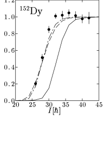
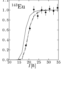
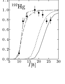
Figure 4: The $\gamma$-ray intensity for decay-out of the yrast SD band in ¹⁵²Dy (left), ¹⁴³Eu (middle) and ¹⁹²Hg (right). The solid, dashed and dot-dashed lines denote the results without any adjustment, with modification by $C_{\rho}$, with modification by $C_{\rm mass}$ (both are explained in the text), respectively. The result with using the “back-shifted level density” with $E_{\rm BS}=1.0$ MeV, is also included as a dotted line for ¹⁹²Hg.

	152Dy		143Eu		192Hg
	I=28	I=32	I=37/2	I=41/2	I=12	I=22
${{\mit\Gamma}_{\rm t}}$	$5.9\times 10^{-5}$	$4.7\times 10^{-6}$	$3.7\times 10^{-5}$	$1.1\times 10^{-5}$	$5.9\times 10^{-5}$	$2.8\times 10^{-6}$
${D_{\rm n}}$	$1.1\times 10^{-5}$	$1.2\times 10^{-5}$	$5.9\times 10^{-4}$	$1.1\times 10^{-3}$	$5.7\times 10^{-6}$	$2.2\times 10^{-5}$
${{\mit\Gamma}_{\rm s}}$	$1.8\times 10^{-8}$	$2.9\times 10^{-8}$	$1.5\times 10^{-9}$	$3.2\times 10^{-9}$	$5.8\times 10^{-11}$	$2.9\times 10^{-9}$
${{\mit\Gamma}_{\rm n}}$	$5.7\times 10^{-9}$	$5.6\times 10^{-9}$	$1.3\times 10^{-9}$	$1.0\times 10^{-9}$	$4.3\times 10^{-9}$	$3.7\times 10^{-9}$
$U^{\prime}_{\rm SDyr}$	4.68	4.61	2.57	2.25	4.24	3.53
$S$	4.0	5.2	4.3	4.9	4.0	5.4
$S(C_{\rm mass})$	5.1	$-$	$-$	3.7	8.2	$-$

Table 2: The calculated values of ${{\mit\Gamma}_{\rm t}},{D_{\rm n}},{{\mit\Gamma}_{\rm s}},{{\mit\Gamma}_{\rm n}}$ and the action $S$ at $U=0$, $I\approx I_{\rm out}^{\rm(cal)}$ and $I_{\rm out}^{\rm(exp)}$, responsible for the decay-out of the yrast SD band. The energy $U^{\prime}_{\rm SDyr}$of the SD yrast states measured from the ND yrast is also listed. The last line lists the value of the action $S$ at $I\approx I_{\rm out}^{\rm(exp)}$ calculated with the collective mass renormalization $C_{\rm mass}=1.4$, 0.7 and 3.0 for ¹⁵²Dy, ¹⁴³Eu and ¹⁹²Hg, respectively. The unit for ${{\mit\Gamma}_{\rm t}},{D_{\rm n}},{{\mit\Gamma}_{\rm s}},{{\mit\Gamma}_{\rm n}}$ and $U^{\prime}_{\rm SDyr}$ is MeV.

As is discussed in the previous sections (see §2.2), the decay-out probability, ${N_{\rm out}}$, and so the $\gamma$-ray intensity, $I_{\gamma}$, is determined by four quantities; the tunneling width, ${{\mit\Gamma}_{\rm t}}$, the electromagnetic decay widths for the SD and ND bands, ${{\mit\Gamma}_{\rm s}}$ and ${{\mit\Gamma}_{\rm n}}$, and the mean level distance of ND states, ${D_{\rm n}}$ (or equivalently the level density, ${\rho_{\rm n}}$). Table 2 shows the values of these quantities responsible for the decay-out, evaluated at $U=0$, $I\approx I_{\rm out}^{\rm(cal)}$ and $I_{\rm out}^{\rm(exp)}$. As for the electromagnetic transition rates, ${{\mit\Gamma}_{\rm s}}$ is that of the stretched E2 and ${{\mit\Gamma}_{\rm n}}$ is of the statistical E1 in the decaying spin region. They are well determined by the equilibrium shape and the excitation energy of the SD band from the ND yrast band, namely by the minima of the calculated potential energy surface. On the other hand, ${{\mit\Gamma}_{\rm t}}$ is calculated by the collective mass tensor and the potential energy barrier, i.e. the behaviour of the saddle point region. Our potential energy surface gives correct equilibrium shape, which is deduced from the measured life time of the SD band, and the calculated barrier also seems to be consistent with other calculations, see for example Refs. [35, 36]. Therefore we do not try any adjustment for quantities related to the potential energy surface in the present work, although there may exist a room for some improvement if we use a different mean-field from the Nilsson potential or a different type or strength for the residual pairing interactions. Remaining quantities in question are the level density and the collective mass parameters. We try to adjust these quantities in order to obtain agreement of the decay-out spin as in the following.

We remark that some additional effects on the level density are not included in the present calculations. For example, the pairing correlation that may be present at relatively low spins may reduce the level density by a factor of up to $\sim 10^{2}$ while the effects of collective vibrations such as beta and gamma modes may increase the level density. To represent these effects and some other origins of ambiguity, we shall allow a renormalization factor of the level density $C_{\rho}$ that multiply the level density ${\rho_{\rm n}}$ of normal deformed states as ${\rho_{\rm n}}\rightarrow C_{\rho}{\rho_{\rm n}}$. Since we explicitly deal with the superdeformed states in the shell model description, we do not apply such a renormalization for the superdeformed states to avoid an inconsistency. The results fitting the decay-out spin by using the factor $C_{\rho}$ are shown by the dashed lines in Fig. 4; the values of which are $C_{\rho}=0.1$, $15$ and $2\times 10^{-4}$, for ¹⁵²Dy, ¹⁴³Eu and ¹⁹²Hg, respectively. It should be mentioned that in the calculation of Ref. [13], the calculated $\gamma$-ray intensity was mistaken by two spin units, i.e. it was $I_{\gamma}(I-2)$; this is the main reason why the $C_{\rho}$ factor is about an order of magnitude smaller in the present calculation than in [13]. The resultant $C_{\rho}$ factor in ¹⁵²Dy and ¹⁴³Eu may be acceptable. But it is too small for ¹⁹²Hg since the ND level spacing at the excitation energy $U^{\prime}\approx 4$ MeV becomes ${D_{\rm n}}\approx 30-100$ keV, which is unphysically large. The fluctuation analysis of the quasi-continuum decay-out transitions in ¹⁹²Hg [46] suggests that the ND level density ${\rho_{\rm n}}$ is smaller than the Fermi gas estimate due to the pairing correlation, and that the reduction of ${\rho_{\rm n}}$ is the order of $10^{-1}-10^{-2}$. As for the level density, the back-shifted Fermi gas formula, namely $U$ is replaced by $(U-E_{\rm BS})$ in Eq. (14), is often used to include the effect of the pairing correlation. In the decay of the Hg region, the decay-out spin is small and this effect may be more important than in the case of the Dy region. Therefore, the results with using $E_{\rm BS}=1.0$ MeV is also included as a dotted line for ¹⁹²Hg in Fig. 4. As seen in the figure, it helps to shift the calculated decay-spin lower by about 3 $\hbar$ but the amount is not enough.

As an another origin of the discrepancy, we consider a possibility that the collective mass could be affected by some additional effects. The essential contents of the pair hopping model is the number of single-particle level crossings and the pairing gap. We have estimated the number of crossings by using a lowest order semiclassical (Fermi-gas) approximation in Eq. (5), and detailed properties of individual nucleus cannot be reflected. However, if one calculate the number of crossing microscopically or take into account the shell effects in the single-particle orbits, this quantity could be largely modified. This may influence the collective mass $m_{ij}(q_{1},q_{2})$. To represent such effects, we introduce a renormalization factor $C_{\rm mass}$ that modifies as $m_{ij}(q_{1},q_{2})\rightarrow C_{\rm mass}\,m_{ij}(q_{1},q_{2})$. It should be noticed that the scaling factor $C_{\rm mass}$ affects the calculated action in two ways: one is a simple scaling of action by a factor $\sqrt{C_{\rm mass}}$ as is clear from Eqs. (9) and (10), the other is a change through the variation of the zero-point energy $\hbar{\omega_{\rm s}}/2$ in the action integral. Both effects make the action larger (smaller) if $C_{\rm mass}>1$ ($<1$). The results fitting the decay-out spin by using the factor $C_{\rm mass}$ are shown by the dot-dashed lines in Fig. 4; the values of which are $C_{\rm mass}=1.4$, $0.7$ and $3.0$, for ¹⁵²Dy, ¹⁴³Eu and ¹⁹²Hg, respectively. As in the case of the introduction of $C_{\rho}$, the factor seems large for Hg.

From the above discussion, it is clear that we have large discrepancy for the decay-out spin value in ¹⁹²Hg. According to the results of more systematic calculation [47] it is one of the worst cases in the $A\approx 190$ nuclei. In this systematic calculation the empirical level density parameters [38] are used so that the results for the intensity data are slightly different from those shown in this paper. Also, the back-shifted level density with $E_{\rm BS}=1.0$ MeV is used for comparison with the data for nuclei in the $A\approx 190$ region. The results of Ref. [47] show that the basic characteristic features of intensity pattern are reproduced in both the $A\approx 150$ and 190 regions; especially the common rapid decrease of transitions at lower spins. The observed decay-out spin is about 25$\hbar$ on average in the $A\approx 150$ region, while it is about 10$\hbar$ in the $A\approx 190$ region. On average calculated decay-out spins are comparable to the observed ones in the $A\approx 150$ region, but those in the $A\approx 190$ region are a little larger than the observed ones systematically even though the back-shift in the level density formula is employed. The calculation reproduces qualitatively the empirical observation that the average decay-out spins in the $A\approx 190$ nuclei are systematically smaller than those in the $A\approx 150$ nuclei, but the amount is not enough. This trend is mainly due to the facts that the calculated action as a function of spin is somewhat different between nuclei in the two regions (see Fig. 2), which reflects the difference in the potential energy surfaces, and that the level density parameter, $a_{\rm n}/A$, is systematically smaller in the $A\approx 190$ region. We have to admit that the calculation overestimates systematically the decay-out spins in the $A\approx 190$ region, which suggests that the calculated action values are too small in these nuclei. It seems that some further mechanisms which discriminate SD bands in these two regions are necessary. Presently we do not have any clue to solve this problem.

3.2 Decay-out of excited superdeformed states

3.2.1 Tunneling width

Let us first discuss the tunneling width ${{\mit\Gamma}_{\rm t}}$ which is the most important quantity in describing the decay-out of excited superdeformed states. As discussed in §2.4, we evaluate the tunneling width with use of Eq. (11), which is expected to give an average behaviour of ${{\mit\Gamma}_{\rm t}}$. In the analysis below, we shall also show results obtained by using Eq. (8), which provides an upper limit of ${{\mit\Gamma}_{\rm t}}$, in order to illustrate the difference in the two evaluations of ${{\mit\Gamma}_{\rm t}}$. The use of Eq. (11) is referred to as the case (a) in the following, while the evaluation of the upper limit with Eq. (8) is as the case (b).

In Fig. 5, we show dependence of the calculated tunneling width on the spin and the excitation energy. The upper three panels show results in the case (a), calculated for the three nuclei, ¹⁵²Dy(left), ¹⁴³Eu(middle) and ¹⁹²Hg(right). The calculated tunneling width ${{\mit\Gamma}_{\rm t}}$ increases exponentially with the excitation energy until the energy reaches the barrier height. Note that the tunneling transmission coefficient $T=1/(1+\exp 2S)$ increases exponentially with excitation energy since the action integral $S$ decreases almost linearly with increasing the excitation energy (cf. §2.5 and Fig. 2). On the other hand, the knocking probability proportional to the level spacing ${D_{\rm s}}$ exhibits an exponential decrease, but this decrease is weaker than the increase in the transmission coefficient. A systematic spin-dependence is also seen in ${{\mit\Gamma}_{\rm t}}$ for the energy region below the barrier height. Namely, the tunneling width for the yrast SD states (corresponding to the thick curve in Fig. 5) decreases exponentially with increasing spin except at high spins ($I\mathop{\vbox{ \offinterlineskip\hbox{$>$}\hbox to7.7778pt{\hss\hbox{$\sim$}\hss}}}30$) in ¹⁹²Hg. The spin-dependence originates mainly from the tunneling transmission coefficient since the spin-dependence in the level density of SD states is weak. As the excitation energy exceeds the barrier height, the calculated tunneling width turns to decrease. This is because the transmission coefficient saturates to a constant value $\approx 1/2$ and the tunneling width ${{\mit\Gamma}_{\rm t}}\approx{{D_{\rm s}}/4\pi}$ then decreases with excitation energy as it is governed by the level spacing ${D_{\rm s}}$ of the excited SD states. In this regime, the tunneling width depends mostly on the excitation energy measured from the SD yrast, but it is insensitive to the spin as the level density ${\rho_{\rm s}}$ of SD states is.

The lower panels show the tunneling width in the case (b) where the knocking frequency is given by the collective vibrational frequency ${\omega_{\rm s}}$. Since ${\omega_{\rm s}}$ depends little on the excitation energy and spin, the energy dependence of the tunneling width is solely governed by the exponential increase of the transmission coefficient below the barrier, and it saturates at ${{\mit\Gamma}_{\rm t}}\approx{\hbar{\omega_{\rm s}}/4\pi}$ above the barrier and becomes spin independent.

Figure 5: The tunneling width ${{\mit\Gamma}_{\rm t}}$ for ¹⁵²Dy (left), ¹⁴³Eu (middle) and ¹⁹²Hg (right) as a function of spin for different excitation energies. The line styles are defined in the same manner as in Fig. 2. The upper three panels show the results in the case (a) using ${{\mit\Gamma}_{\rm t}}=({D_{\rm s}}/2\pi)T$ whereas the lower panels show those in the case (b) calculated with ${{\mit\Gamma}_{\rm t}}=(\hbar{\omega_{\rm s}}/2\pi)T$. The signature and parity is the same as in Fig. 2.

Comparing the two cases quantitatively, it is seen that the tunneling width in the case (a) is significantly smaller than that in the case (b) by more than the order of $10^{2}$ for the excitation energy $E_{\rm ex}=2\sim 3$ MeV and the difference increases further as $E_{\rm ex}$ reaches near and above the barrier. (Note, however, that the value of ${{\mit\Gamma}_{\rm t}}$ in the case (b) for the energy above the barrier height is not meaningful since Eq. (8) does not give correct description of the statistical mixing that is expected above the barrier.) We see also that the difference of ${{\mit\Gamma}_{\rm t}}$ between the two cases is not significant at the low excitations near the yrast SD states ($E_{\rm ex}\mathop{\vbox{ \offinterlineskip\hbox{$<$}\hbox to7.7778pt{\hss\hbox{$\sim$}\hss}}}1$ MeV). This is because ${D_{\rm s}}$ in this energy region is of the same order as $\hbar{\omega_{\rm s}}\sim 1.0$ MeV.

3.2.2 Decay-out properties

Figure 6 shows the calculated average decay-out branching ratio ${N_{\rm out}}$ in ¹⁵²Dy. The value of ${N_{\rm out}}$ is plotted as a function of spin $I$ for different excitation energies $E_{\rm ex}=1.0,2.0$ and $3.5$ MeV measured from the SD potential minimum $E_{\rm SD}^{0}$. A steep increase of ${N_{\rm out}}$ with decreasing $I$ around ${N_{\rm out}}\sim 1/2$ indicates a sharp decay-out, and this feature is commonly seen for all excitation energies. As the excitation energy increases, the decay-out occurs at higher spins. This is because the tunneling probability increases. In Fig. 6, we also show ${N_{\rm out}}$ calculated with use of Eq. (8) (the case (b)) with thin lines. The difference between the two cases (a) and (b) is significant for high excitation energy $E_{\rm ex}\mathop{\vbox{ \offinterlineskip\hbox{$>$}\hbox to7.7778pt{\hss\hbox{$\sim$}\hss}}}2$ MeV because of the difference in ${{\mit\Gamma}_{\rm t}}$ becomes large as discussed above. On the other hand, the two evaluations give similar results for $E_{\rm ex}\mathop{\vbox{ \offinterlineskip\hbox{$<$}\hbox to7.7778pt{\hss\hbox{$\sim$}\hss}}}1$ MeV.

Figure 6: The average decay-out probability ${N_{\rm out}}(E,I)$ plotted as a function of spin, calculated for ¹⁵²Dy $((\alpha,\pi)=(0,+))$ with $C_{\rho}=0.1$. The thick solid, dashed and dot-dashed lines indicate the results in the case (a) using ${{\mit\Gamma}_{\rm t}}=({D_{\rm s}}/2\pi)T$ for excitation energies $E_{\rm ex}=1.0$, 2.0 and 3.5 MeV, respectively. Thin lines represent the results in the case (b) employing ${{\mit\Gamma}_{\rm t}}=(\hbar{\omega_{\rm s}}/2\pi)T$.

The decay-out branching ratio ${N_{\rm out}}$ modifies the E2 transition probability of exited superdeformed states as described in §2.4. The energy levels $E_{\alpha}(I)$ of SD states and the E2 transition probabilities $\tilde{S}_{\alpha I,\beta I-2}$ calculated for ¹⁵²Dy are plotted in Fig. 7. In this figure shown are such strong E2 transitions that satisfy $\tilde{S}_{\alpha I,\beta I-2}>1/\sqrt{2}$ by connecting the energy levels with solid lines. Compared with the previous calculation which does not include the decay-out effect (Fig. 6 in Ref. [18]), strong E2 transitions disappear at low spin and high excitation energy due to the decay-out to normal deformed states. The sequence of strong E2 transitions associated with the yrast SD states correspond to the yrast SD rotational band, and the figure shows that the yrast SD band decays out around $I=28$ (See also Fig. 4). There exist several rotational bands above the yrast band up to the excitation energy $U\mathop{\vbox{ \offinterlineskip\hbox{$<$}\hbox to7.7778pt{\hss\hbox{$\sim$}\hss}}}2$ MeV. The decay-out spin of these bands is higher than that of the yrast bands since the decay-out branching ratio ${N_{\rm out}}$ increases with excitation energy.

Figure 7: The energy levels of the yrast and excited SD states, shown with horizontal bars, calculated for ¹⁵²Dy ($(\alpha,\pi)=(0,+)$) by means of the cranked shell model diagonalization. A rigid body rotational energy $E_{\rm rigid}=I(I+1)/{\cal J}_{\rm rigid}$ is subtracted. Solid lines connecting the energy levels indicates strong E2 transitions satisfying $\tilde{S}_{\alpha I,\beta I-2}>1/\sqrt{2}$.

Since the decay-out occurs at the spin where ${N_{\rm out}}$ increases sharply from zero and reaches to ${N_{\rm out}}\approx 1/2$, it is possible to define the decay-out spin ${I_{\rm out}}(U)$ for a given excitation energy $U$ by means of a condition ${N_{\rm out}}=1/2$. This definition of the decay-out spin is slightly different from that used in §3.1 to describe the decay-out of the yrast SD band (It was defined there by $\prod_{I^{\prime}}(1-{N_{\rm out}}(I^{\prime}))=1/2$). However, the actual difference is less than $2\hbar$ for the value of the decay-out spin, and in the following discussion we adopt the condition ${N_{\rm out}}=1/2$ as the definition of the decay-out of excited superdeformed states. Since ${N_{\rm out}}$ is a function of the spin $I$ and the energy $E$, the criterion ${N_{\rm out}}=1/2$ gives a boundary in the $(E,I)$ plane. We can represent the decay-out boundary also in terms of the decay-out energy ${E_{\rm out}}(I)$ as a function of spin $I$ as well as the decay-out spin ${I_{\rm out}}(U)$.

The decay-out energy ${E_{\rm out}}(I)$ calculated for ¹⁵²Dy is shown in Fig. 8. Results in the left panel is obtained with no adjustment of the level density nor of the mass parameter. In this figure, we show not only the results in the case (a), evaluated by using ${{\mit\Gamma}_{\rm t}}={({D_{\rm s}}/2\pi)}T$, Eq. (11), which gives the average behaviour of the decay-out, but also two other results in the cases (a’) and (b). In the case (a’) we assumed ${{\mit\Gamma}_{\rm t}}={D_{\rm s}}T$ that gives the tunneling width different from that in the case (a) by a factor of $2\pi$. Comparing the results in the two cases (a) and (a’), we see that the ambiguity in the numerical factor of the tunneling width (difference of the factor $2\pi$) does not cause large difference in the decay-out boundary. In the case (b), on the other hand, we evaluate with use of the other expression ${{\mit\Gamma}_{\rm t}}={(\hbar{\omega_{\rm s}}/2\pi)}T$, Eq. (8), which is expected to give an upper limit of ${{\mit\Gamma}_{\rm t}}$. The decay-out energies ${E_{\rm out}}(I)$ for the two cases (a) and (b) differ by several hundred keV at maximum, and the difference is larger than the ambiguity of a numerical factor in the cases (a) and (a’). We can conclude from these comparisons that the reduction of the knocking probability (the factor $\sim{D_{\rm s}}/{\omega_{\rm s}}$ in Eq. (11) v.s. Eq. (8)) plays important roles for the description of the excited SD states.

Figure 8: Left panel: Decay-out energy ${E_{\rm out}}(I)$ for ¹⁵²Dy ($(\alpha,\pi)=(0,+)$) as a function of spin $I$, together with the barrier height ${V_{\rm b}}$ and the ND yrast energy $E_{\rm NDyr}$. All these quantities measured the SD yrast energy $E_{\rm SDyr}$ are plotted. The decay-out energy are shown in the three cases, (a) ${{\mit\Gamma}_{\rm t}}=({D_{\rm s}}/2\pi)T$, (a’) ${{\mit\Gamma}_{\rm t}}={D_{\rm s}}T$ and (b) ${{\mit\Gamma}_{\rm t}}=(\hbar{\omega_{\rm s}}/2\pi)T$. The calculation is done without any adjustment of the ND level density and the collective mass. Middle panel: The onset energy of rotational damping ${E_{\rm damp}}(I)$ is plotted together with the boundary energy for the SD-ND mixing defined by ${{\mit\Gamma}_{\rm t}}/{D_{\rm n}}=1$ and the decay-out energy ${E_{\rm out}}$, calculated in the case (a) with $C_{\rho}=0.1$. The three regions separated by the two boundaries ${E_{\rm out}}(I)$ and ${E_{\rm damp}}(I)$ are indicated as “pure rotational band”,“damped rotation”, and “ND dominant compound” (see text). Right panel: Same as the middle except for the adjustment of the collective mass with $C_{\rm mass}=1.4$.

The decay-out boundary for the zero excitation energy $U=0$ corresponds to the decay-out of the yrast SD band. As the excitation energy increases, the decay-out boundary moves to higher spins. In other words, the decay-out of excited superdeformed states takes place at higher spin than that of the yrast SD band. The calculation indicates that the decay-out spin ${I_{\rm out}}(U)$ increases by about $8\hbar$ for increasing excitation energy by 1 MeV. Equivalently the decay-out energy ${E_{\rm out}}(I)$ increases monotonically with increasing spin. The slope of the decay-out energy ${E_{\rm out}}(I)$ is larger than that of the barrier height ${V_{\rm b}}(I)$ since the decay-out probability ${N_{\rm out}}$ depends not only on the tunneling transmission coefficient but also on other quantities such as the level density of ND states, which vary strongly with spin.

The decay-out spin for $U=0$ is seen in the figure to be ${I_{\rm out}}(U=0)\approx 30\hbar$, which is slightly larger than the experimental decay-out spin of the yrast SD band. In order to have more reliable description, we have discussed in §3.1 two ways of adjustment by introducing the renormalization factor $C_{\rho}$ of the ND level density and by the renormalization $C_{\rm mass}$ of the collective mass parameter. In the middle (right) panel, we show the decay-out boundary for the excited SD states, evaluated in the case (a), with use of the adjusted ND level density with $C_{\rho}=0.1$ (the adjusted collective mass parameter $C_{\rm mass}=1.4$). Since the renormalization factors $C_{\rho}$ and $C_{\rm mass}$ are not very different from unity, difference between the left and middle (right) panels is not large. The difference between the two adjustments (middle vs. right panels) is very small for the lower energy region $U\mathop{\vbox{ \offinterlineskip\hbox{$<$}\hbox to7.7778pt{\hss\hbox{$\sim$}\hss}}}2$ MeV since the decay-out spin of the yrast SD band is adjusted in both cases. The difference, however, is not negligible for higher energy region, especially for the region above the barrier height. The renormalization of the collective mass affects the decay-out property only below the barrier, while the renormalization of the ND level density influences both below and above the barrier.

In order to clarify the decay-out properties, it is useful to recall that the average decay-out probability ${N_{\rm out}}$ is a function of two ratios ${{\mit\Gamma}_{\rm t}}/{D_{\rm n}}$ and ${{\mit\Gamma}_{\rm s}}/{{\mit\Gamma}_{\rm n}}$ [11, 13]. We found that the behavior of the decay-out energy ${E_{\rm out}}$ is mainly governed by the ratio ${{\mit\Gamma}_{\rm t}}/{D_{\rm n}}$. To show this, we plot in the middle and right panels of Fig. 8 a boundary energy that is defined by the condition ${{{\mit\Gamma}_{\rm t}}/{D_{\rm n}}}=1$, and compare with the decay-out energy ${E_{\rm out}}(I)$. If the ratio ${{{\mit\Gamma}_{\rm t}}/{D_{\rm n}}}$ is more than 1, it implies that a significant amount of components of ND states mix into SD states. The condition ${{{\mit\Gamma}_{\rm t}}/{D_{\rm n}}}=1$ defines a boundary for the strong mixing among SD and ND states. It is seen from the figure that the boundary of strong mixing follows rather well with the decay-out energy ${E_{\rm out}}(I)$. The ratio of the electromagnetic transition widths ${{\mit\Gamma}_{\rm s}}/{{\mit\Gamma}_{\rm n}}$ plays a relatively minor role in determining the spin and excitation energy dependence of the decay-out, especially for the spin region much higher than the decay-out spin of the yrast SD band. For the high spins, the E2 decay width of ND states dominates over the E1 decay width, and the ratio of electromagnetic widths ${{\mit\Gamma}_{\rm s}}/{{\mit\Gamma}_{\rm n}}$ is approximated by $\left(Q_{\rm s}/Q_{\rm n}\right)^{2}\times\left({{\cal J}_{\rm n}}/{{\cal J}_{\rm s}}\right)^{5}$, where ${Q_{\rm s}}$ (${Q_{\rm n}}$) and ${{\cal J}_{\rm s}}$ (${{\cal J}_{\rm n}}$) are the static quadrupole moment and moment of inertia for the SD (ND) states. The ratio then depends neither on excitation energy nor spin, and takes a value which is a little more than 1 but does not exceed $10^{1}$.

The decay-out boundary ${E_{\rm out}}(I)$ in the region above the barrier height shows behaviour different from that below the barrier. As seen in the middle panel (and also in Figs. 9 for ¹⁴³Eu and 10 for ¹⁹²Hg), the boundary rises very sharply above the barrier. In the region above the barrier the SD and ND states mix statistically to form compound states as the ratio ${{\mit\Gamma}_{\rm t}}/{D_{\rm n}}$ reduces to the ratio of the level spacings ${D_{\rm s}}/{D_{\rm n}}$ of SD and ND states. (Note that the results of the cases (a) or (a’) should be adopted for the region above the barrier since the case (b) is not applicable in this region.) As spin increases, the ND yrast energy relative to the SD yrast becomes higher and the ratio ${{\mit\Gamma}_{\rm t}}/{D_{\rm n}}\sim{D_{\rm s}}/{D_{\rm n}}={\rho_{\rm n}}/{\rho_{\rm s}}$ decreases exponentially for a fixed value of $U$. In other words, superdeformed states become dominant components of the statistically mixed compound states. On the other hand, the ratio ${{\mit\Gamma}_{\rm s}}/{{\mit\Gamma}_{\rm n}}$ increases with spin since the E2 decay probability ${{\mit\Gamma}_{\rm s}}$ associated with SD states becomes larger due to the $E_{\gamma}^{5}$ factor while the ND decay width ${{\mit\Gamma}_{\rm n}}$ decreases due to the decrease of the relative excitation energy. Both two effects, the decrease in ${{\mit\Gamma}_{\rm t}}/{D_{\rm n}}\sim{D_{\rm s}}/{D_{\rm n}}$ and the increase in ${{\mit\Gamma}_{\rm s}}/{{\mit\Gamma}_{\rm n}}$, favor dominance of the SD transitions at very high spins while the ND transitions dominates at lower spins. The decay-out spin above the barrier height represents a border where the relative dominance of the SD and ND transitions is interchanged.

3.2.3 Rotational damping effects

Let us now discuss effects of the rotational damping on the excited superdeformed states. As seen in Fig. 7, The strong E2 transitions with $\tilde{S}_{\alpha I,\beta I-2}>1/\sqrt{2}$ gradually disappear in the region with excitation energy $U$ greater than about 2 MeV. This disappearance of the strong E2 transitions is caused by the rotational damping. Although the transition from the rotational band structures seen near the yrast line to the rotational damping in the highly excited states is gradual, let us characterize it by introducing a boundary energy for the onset of rotational damping. For this purpose, we calculate the branching number ${n_{\rm branch}}=(\sum_{\beta}S_{\alpha I,\beta I-2}^{2})^{-1}$ [4, 18, 19] that quantifies the fragmentation of E2 decay from a SD state $\alpha$ at spin $I$. The onset energy of damping ${E_{\rm damp}}(I)$ is then defined as the energy where the average branching number calculated as a function of the energy $E$ exceeds 2 for a given spin $I$. The calculation of ${E_{\rm damp}}(I)$ is the same as in Ref. [18, 19]. The onset energy ${E_{\rm damp}}(I)$ of the rotational damping is plotted in the middle and right panels of Fig. 8.

Using the decay-out energy ${E_{\rm out}}(I)$ and the onset energy ${E_{\rm damp}}(I)$ of rotational damping, the excited superdeformed states are divided into three regions. The E2 transitions associated with the superdeformed states can exist only in the low energy region below the decay-out boundary ${E_{\rm out}}(I)$ or at the high spin side of this boundary. This region is further divided into two by the second boundary ${E_{\rm damp}}(I)$. Below ${E_{\rm damp}}(I)$, the superdeformed states form the rotational band structures, i.e., sequences of levels connected by the strong E2 transitions. The superdeformed rotational bands are confined in this region, which is labeled in Fig. 8 with “pure rotational band”. On the other hand, concerning the excited SD states which are located above ${E_{\rm damp}}(I)$ and at the high spin side of the decay-out boundary ${E_{\rm out}}(I)$, they decay also by the rotational E2 transitions characteristic to the SD shape, but the the rotational E2 transitions are fragmented (i.e. the rotational damping) due to the admixture of superdeformed many-particle many-hole configurations caused by the residual interaction. This second region is labeled in Fig. 8 with “damped rotation”. Note that the damped E2 transitions can be found even above the barrier. The third region that is situated at low-spin side (and high energy side) of the decay-out boundary ${E_{\rm out}}(I)$ is labeled with “ND dominant compound” in Fig. 8. The SD states in this region mix strongly with the ND states, and the decay of these states are dominated by the E1 or E2 transitions associated with the ND states.

We may use the onset energy ${E_{\rm damp}}(I)$ as a guideline of whether the excited superdeformed states have character of compound states. At excitation energy higher than ${E_{\rm damp}}(I)$, the SD states become strong admixture of different SD $n$p-$n$h configurations. Thus it may be justified to use the average estimate of the tunneling width, given by Eq. (11) (the case (a) with the knocking frequency $\propto{D_{\rm s}}$), for the energy region sufficiently higher than ${E_{\rm damp}}(I)$. But for the energy region below ${E_{\rm damp}}(I)$, we can expect possible fluctuation around the average estimate. As discussed above, an upper-limit estimate of the fluctuation is given by Eq. (8) (the case (b)). Note, however, that the ambiguity due to the fluctuation is not large in this energy region since the difference in the decay-out boundary ${E_{\rm out}}(I)$ between the two cases is small (see the left panel of Fig. 8).

3.2.4 ¹⁴³Eu

Figure 9: Same as Fig. 8 but for ¹⁴³Eu ($(\alpha,\pi)=(1/2,+)$) with $C_{\rho}=15.0$ (middle panel) and with $C_{\rm mass}=0.7$ (right panel)

Figure 9 shows the results for ¹⁴³Eu. Basic features are found similar to those in ¹⁵²Dy. The influence of the adjustment of the ND level density (the middle panel with $C_{\rho}=15.0)$ and of the collective mass parameter (the right panel with $C_{\rm mass}=0.7$) on the decay-out boundary is not large, likewise in the case of ¹⁵²Dy. There exits also in this nucleus the three regions classified in terms of the decay-out and the onset of the rotational damping, as shown in the middle and right panels. A remarkable difference from ¹⁵²Dy is that the decay-out boundary is located at lower spin by about $10\hbar$. The low values of decay-out spin is seen not only for the yrast SD states $U=0$ (as discussed in §3.1) but also for the highly excited SD states including the states above the barrier. Consequently the region of “damped rotation” is much larger than in ¹⁵²Dy. The calculation predicts the decay-out spin ${I_{\rm out}}\sim 35-45\hbar$ for the highly excited SD states above the barrier height. The SD states lying $I\mathop{\vbox{ \offinterlineskip\hbox{$>$}\hbox to7.7778pt{\hss\hbox{$\sim$}\hss}}}35-45\hbar$ and $U\mathop{\vbox{ \offinterlineskip\hbox{$>$}\hbox to7.7778pt{\hss\hbox{$\sim$}\hss}}}2$ MeV emit characteristic rotational E2 gamma-rays with fragmentation caused by the rotational damping. This feature seems consistent, at least qualitatively, with the experimental observation of intense quasi-continuum E2 transitions [10].

3.2.5 ¹⁹²Hg

Figure 10: Left panel: Calculated decay-out energies ${E_{\rm out}}(I)$ in the cases (a) and (b) (see text) for ¹⁹²Hg ($(\alpha,\pi)=(0,+)$) calculated with no adjustments ($C_{\rho}=1,C_{\rm mass}=1$), plotted together with the onset energy of rotational damping ${E_{\rm damp}}(I)$, the boundary energy for the SD-ND mixing defined by ${{\mit\Gamma}_{\rm t}}/{D_{\rm n}}=1$ calculated in the case (a), the barrier height ${V_{\rm b}}$ and the ND yrast energy $E_{\rm NDyr}$. Middle panel: The decay-out energies ${E_{\rm out}}(I)$ in the case (a), calculated with the level density renormalization $C_{\rho}=2.0\times 10^{-4}$. Right panel: The decay-out energies ${E_{\rm out}}(I)$ in the case (a), calculated with the collective mass renormalization $C_{\rm mass}=3.0$ and the boundary energy for the SD-ND mixing.

Figure 10 shows the results for ¹⁹²Hg. Although there are some common features to those in ¹⁵²Dy and ¹⁴³Eu, large differences are observed. The left panel shows the results without any adjustment. It is seen that difference between the case (a) and the case (b) is larger than in ¹⁵²Dy and ¹⁴³Eu. This is because the spin dependence of the tunneling width ${{\mit\Gamma}_{\rm t}}$ is much weaker than in ¹⁵²Dy and ¹⁴³Eu as seen in Fig. 5, hence the difference in ${{\mit\Gamma}_{\rm t}}$ (the cases (a) vs. (b)) causes larger change in the decay-out boundary. Weak spin-dependence is also seen in the barrier height. These features are due to the qualitative difference of the calculated potential energy surface between the Dy and Hg nuclei, which is stressed at the end of §2.5. It is also noted that the decay-out boundary above the barrier is located at rather low spin ($I\approx 40\hbar$). This is caused by the relatively high level density of the superdeformed states in this nucleus. (The corresponding level density parameter is a=A/13.0 MeV^-1.) An unwanted feature in the left panel is that the theoretical prediction of the decay-out spin for the yrast SD band is significantly higher than that observed in the experiment by more than $10\hbar$ as already discussed in §3.1.

In §3.1, we introduced two ways of adjustment by renormalizing the level density of ND states by a factor $C_{\rho}=2.0\times 10^{-4}$ and by renormalizing the collective mass parameter by $C_{\rm mass}=3.0$. The results of these calculations are shown in the middle and right panels. Remarkably large difference between the two calculations is seen for the decay-out boundary of the excited SD sates although both are adjusted to reproduce the observed decay-out of yrast SD band. The change in the collective mass parameter increases the action value of the tunneling path by a factor of 1.9$-$2.1 and reduces the tunneling transmission coefficient, but it does not influence the behavior above the barrier where the tunneling action becomes zero. On the other hand, the change in the ND level density influences both below and above the barrier. Since the renormalization factor for the adjusted ND level density ($C_{\rho}=2.0\times 10^{-4}$) is very small, its effect is drastic. For example, the decay-out boundary above the barrier is largely shifted to $I\approx 20\hbar$, which is very different from the decay-out boundary calculated with the adjusted collective mass ($C_{\rm mass}=3.0$). Note, however, that the modification of the ND level density with the factor of $10^{-4}$ may not be realistic, although it is also not certain whether the renormalization of the collective mass parameter by a factor of 3 is justified. We can say that the decay-out boundary has different spin dependence and stays at considerably lower excitation energy in ¹⁹²Hg compared to ¹⁵²Dy and ¹⁴³Eu if a realistic ND level density is used, and this is mainly due to the fact that the barrier height in the $A\approx 190$ nuclei saturates or even decrease gradually at $I\mathop{\vbox{ \offinterlineskip\hbox{$>$}\hbox to7.7778pt{\hss\hbox{$\sim$}\hss}}}20-30\hbar$.

3.3 Number of rotational bands

As Fig. 7 illustrates, the number of superdeformed rotational bands existing in a nucleus is limited to a finite number since the rotational E2 transitions associated with highly excited levels exhibit the rotational damping. In addition, the decay-out transitions are present at low spins. Since the rotational band structures are not observed if the decay-out probability dominates over the E2 transitions, the decay-out further reduces the number of rotational bands especially at low spins where the decay-out plays a role. An effective number of decay paths, which approximately gives the number of superdeformed rotational bands, has been evaluated experimentally from analysis of the quasi-continuum E2 gamma-rays in superdeformed nuclei [2, 9, 48]. In contrast to the intensity data for the decay-out of yrast SD bands, where the tunneling probability in a narrow spin-range is relevant because of the sharp decay-out, the number of rotational band is sensitive to the decay-out process in a broad spin-range, as is shown in the following, and is effective to study the barrier penetration problem. We, therefore, adopt in this subsection the number of rotational bands as a typical observable on the excited superdeformed states, and discuss in detail effects of the decay-out on this quantity.

The number of superdeformed rotational bands, ${N_{\rm band}}$, is evaluated as follows. To make a distinction between the levels forming rotational bands and those exhibiting the rotational damping, we consider the branching number of E2 transitions ${n_{\rm branch}}=\left(\sum_{\beta}S_{\alpha I,\beta I-2}^{2}\right)^{-1}$ defined for each SD state $\alpha$ at spin $I$. The effect of the decay-out on this quantity is taken into account by means of Eq. (2). Namely, the branching number is now given by

$$\tilde{n}_{\rm branch}(\alpha,I) = \left(\sum_{\beta}\tilde{S}_{\alpha I,\beta I-2}^{2}\right)^{-1}$$ (19)

$$= (1-{N_{\rm out}}(E_{\alpha},I))^{-2}{n_{\rm branch}}(\alpha,I)$$ (20)

by multiplying the factor $(1-{N_{\rm out}}(E_{\alpha},I))^{-2}$ to the original branching number ${n_{\rm branch}}$. The modified branching number takes a very large value if the decay-out transition is dominant (i.e. ${N_{\rm out}}\approx 1$). The condition $\tilde{n}_{\rm branch}<2$ gives a definition of the states having strong E2 transitions forming superdeformed rotational bands. For fixed spin and parity, we count the excited superdeformed levels that satisfy $\tilde{n}_{\rm branch}<2$ for consecutive two steps of strongest E2 transitions [4, 5, 18, 19]. Summing over four combinations of parity and signature quantum numbers, we evaluate the number of superdeformed rotational bands ${N_{\rm band}}$.

Figure 11: The number of SD rotational bands, ${N_{\rm band}}$, for ¹⁵²Dy, calculated in the two cases (a) and (b) (see text) with $C_{\rho}=0.1$ and plotted as a function of spin $I$. Also shown are the result with $C_{\rm mass}=1.4$ in the case (a) and the one without the decay-out effect.

We show in Fig. 11 the number of superdeformed rotational bands calculated for ¹⁵²Dy. Here we plot ${N_{\rm band}}$ obtained with the renormalization of the ND level density ($C_{\rho}=0.1$) and of the collective mass parameter ($C_{\rm mass}=1.4$) that are chosen to reproduce the decay-out spin of the yrast SD band (cf. §3.1). The average estimate of the tunneling width ${{\mit\Gamma}_{\rm t}}=({D_{\rm s}}/2\pi)T$ (the case (a)) is adopted. The result without the decay-out is also plotted for comparison, which is the same as that obtained in the previous paper [18]. We find that the effect of decay-out reduces significantly the number of bands for the spin region $I\mathop{\vbox{ \offinterlineskip\hbox{$<$}\hbox to7.7778pt{\hss\hbox{$\sim$}\hss}}}50\hbar$. This behavior is easily understood from Figs. 7 and 8. Since the decay-out boundary cuts the region of pure rotational bands at $I\sim 26$ for $U=0$ (yrast states) and at $I\sim 50$ for $U\sim{E_{\rm damp}}$, the effect of the decay-out on ${N_{\rm band}}$ become sizable in the spin region $I\approx 26-50\hbar$. At high spins $I\mathop{\vbox{ \offinterlineskip\hbox{$>$}\hbox to7.7778pt{\hss\hbox{$\sim$}\hss}}}50$ where ${E_{\rm out}}(I)$ exceeds ${E_{\rm damp}}(I)$, the decay-out has little influence on ${N_{\rm band}}$. There is only minor difference between the two ways of renormalization. In the figure we plot also ${N_{\rm band}}$ obtained with the upper limit estimate of ${{\mit\Gamma}_{\rm t}}=(\hbar{\omega_{\rm s}}/2\pi)T$ (the case (b)). The case (b) can be considered to provides a lower limit for the evaluated ${N_{\rm band}}$. The difference in ${N_{\rm band}}$ between the two cases (a) and (b) is up to about by $10\sim 15$. The number of bands is as much as $50-60$ for long spin interval $I\sim 45-60$. It is emphasized that this number is larger than those for ND rare-earth nuclei (${N_{\rm band}}\sim 30$), indicating that the shell effect leading to the large value of ${N_{\rm band}}$ [18, 19] remains even with the presence of the decay-out effect.

Figure 12 shows the results for ¹⁴³Eu. Here the experimental data [48] are compared. To make a direct comparison, we plot ${N_{\rm band}}$ as a function of the E2 gamma-ray energy. The transformation from the spin to the gamma-ray energy is done by calculating the average gamma-ray energy calculated over all E2 transitions as a function of spin. We show the calculated results for both cases (a) and (b). The difference between (a) and (b) and also the difference between the two renormalizations are found smaller than that in ¹⁵²Dy, and it is not more than the size of experimental error bars. The decay-out has little influence on the number of bands for spin region $I\mathop{\vbox{ \offinterlineskip\hbox{$>$}\hbox to7.7778pt{\hss\hbox{$\sim$}\hss}}}50$ ($E_{\gamma}\mathop{\vbox{ \offinterlineskip\hbox{$>$}\hbox to7.7778pt{\hss\hbox{$\sim$}\hss}}}1400$ keV). Gradual decrease of number of bands with decreasing spin in the spin region $I\mathop{\vbox{ \offinterlineskip\hbox{$<$}\hbox to7.7778pt{\hss\hbox{$\sim$}\hss}}}50$ ($E_{\gamma}\mathop{\vbox{ \offinterlineskip\hbox{$<$}\hbox to7.7778pt{\hss\hbox{$\sim$}\hss}}}1400$ keV) is the decay-out effect. Note that with the decay-out effect we obtain overall agreements between the calculated results and the experimental data. The agreement is satisfactory although it is not perfect. We may need more precise comparison using simulated gamma-ray cascades if we want to evaluate the differences between the theories and the experiment.

Figure 12: Same as Fig. 11 but for ¹⁴³Eu. Here ${N_{\rm band}}$ is calculated either with the adjusted $C_{\rho}=15.0$ or with the mass renormalization $C_{\rm mass}=0.7$. It is plotted as a function of the average gamma-ray energy $E_{\gamma}$, and compared with the experimental effective number of decay-path [48].

Figure 13: The calculated ${N_{\rm band}}$ for ¹⁹²Hg. The results with $C_{\rho}=C_{\rm mass}=1$ using formula (a) and (b) are plotted by a thick solid line and a thin dotted one, respectively. Those using (a) with the fitted $C_{\rho}$ and the fitted $C_{\rm mass}$ are plotted by a thick dashed line and a thick dot-dashed one, respectively. They are compared with the number of bands without considering the decay-out effect(a thin solid line).

Finally we show in Fig. 13 the calculated number of bands for ¹⁹²Hg. We plot here four kinds of result; the calculations where no adjustment of the ND level density nor of the collective mass is introduced but we evaluate ${N_{\rm band}}$ in two ways (the case (b) as well as the case (a)), the calculation where the renormalization of the ND level density with $C_{\rho}=2.0\times 10^{-4}$ is taken into account (in the case (a)), and the calculation with the adjustment of the collective mass ($C_{\rm mass}=3.0$) instead of the ND level density. In parallel to the results shown in Fig. 10, significant differences in ${N_{\rm band}}$ are seen among these calculations. Concerning the calculation without any adjustment ($C_{\rho}=C_{\rm mass}=1$), the effect of decay-out is significant and ${N_{\rm band}}$ takes a very small number. However, since this calculation fails to reproduce the decay-out of the yrast SD band, it should be an underestimate. On the other hand, when we make the adjustments to reproduce the yrast decay-out, the results depend very strongly on the method of adjustment. When we adjust the level density of ND states ($C_{\rho}=2.0\times 10^{-4}$), the resultant ${N_{\rm band}}$ takes the value of more than 100 for $I\mathop{\vbox{ \offinterlineskip\hbox{$>$}\hbox to7.7778pt{\hss\hbox{$\sim$}\hss}}}20$. This is because the decay-out occurs only at very low spins, $I\mathop{\vbox{ \offinterlineskip\hbox{$<$}\hbox to7.7778pt{\hss\hbox{$\sim$}\hss}}}20$, even at high excitation energy (Fig. 10), and the large value of ${N_{\rm band}}$ originating from the shell effect [19] remains. When we perform the adjustment with the collective mass ($C_{\rm mass}=3.0$), on the other hand, the decay-out effect influences ${N_{\rm band}}$ in the whole interval of spin, and reduces ${N_{\rm band}}$ significantly taking a value less than 70.

It has been found in Ref. [19] that an extraordinary large ${N_{\rm band}}$ due to the shell effect on the rotational damping has been predicted (also shown in Fig. 13). However, the present result with including the decay-out process suggests the dramatic reduction if we use a realistic ND level density and believe the behaviour of the potential energy surface at higher-spin region. This is mainly because the barrier height of ¹⁹²Hg is lower at higher spins and consequently the decay-out boundary is relatively low in excitation energy as is discussed in §3.2.5. This fact clearly shows that the effect of barrier penetration is crucial in this nucleus, and suggests a possibility to study a large-scale change of the potential energy surface as a function of angular momentum. Experimental information on ${N_{\rm band}}$ would be of crucial importance in this respect.

4 Conclusions

We have constructed a microscopic model of thermally excited superdeformed states that can describe both the rotational damping caused by the residual two-body interaction and the decay-out associated with the barrier penetration to normal deformation. Combining the cranked Nilsson-Strutinsky model for the deformed rotating mean-field, the shell-model description of individual excited superdeformed states, and the the pair hopping mass for the quadrupole shape transition, we define the model microscopically without any phenomenological fitting. The calculations have been done for representative superdeformed nuclei ¹⁵²Dy and ¹⁴³Eu in the $A\approx 150$ region, and ¹⁹²Hg in the $A\approx 190$ region.

The model thus constructed is applied to the decay-out of the yrast superdeformed states to check its validity. The sharpness of the observed decay-out is described well, and a good quantitative account of the decay-out spin is achieved for ¹⁵²Dy and ¹⁴³Eu. However, the model fails to describe the decay-out spin in¹⁹²Hg. We examined possible origins of the discrepancy in connection with the level density of normal deformed states and the collective mass parameter.

We discussed in detail decay-out properties of the excited superdeformed states having the thermal excitation energy up to several MeV above the yrast state. For this purpose, we extended the decay-out theory of Vigezzi et al. [11] by using the prescription of Bjørnholm and Lynn [31]. The calculation shows that the excited superdeformed states decay out at much higher spins than the decay-out spin of the yrast SD bands.

In terms of the decay-out and the onset of the rotational damping, the excited superdeformed states are classified into three groups having different transitional properties; the levels that decay with rotational E2 transitions and form the rotational band structure, the levels that decay with rotational E2 but exhibit the rotational damping, and the others that mix strongly with ND compound levels and decays to ND levels. The model predicts that both the decay-out and the rotational damping influence significantly the effective number of superdeformed bands, an observable for the excited superdeformed states obtained recently by means of the quasi-continuum spectroscopy. The decay-out causes a characteristic decrease in the effective number of superdeformed band with decreasing spin. The study of thermally excited superdeformed bands gives us an opportunity to investigate a large-scale shape dynamics as well as the damping of collective rotational motion.

References

- [1] B. Lauritzen, T. Døssing, and R. A. Broglia, Nucl. Phys. A457 (1986) 61.
-
[2]
B. Herskind,
A. Bracco, R. A. Broglia, T. Døssing, A. Ikeda, S. Leoni, J. Lisle,
M. Matsuo, and E. Vigezzi,
Phys. Rev. Lett. 68 (1992) 3008.
T. Døssing, B. Herskind, S. Leoni, A. Bracco, R. A. Broglia, M. Matsuo, E. Vigezzi, Phys. Rep. 268 (1996) 1. -
[3]
S. Åberg, Phys. Rev. Lett. 64(1990)3119;
S. Åberg, Prog. Part. Nucl. Phys. vol. 28 (Pergamon, 1992) p. 11. - [4] M. Matsuo, T. Døssing, E. Vigezzi, R. A. Broglia, and K. Yoshida, Nucl. Phys. A617 (1997) 1.
- [5] A. Bracco, P. Bosseti, S. Frattini, E. Vigezzi, S. Leoni, T. Døssing, B. Herskind, M. Matsuo, Phys. Rev. Lett. 76 (1996) 4484.
-
[6]
P. J. Twin, Proc. Intern. Conf. on Nuclear
shapes (World Scientific, 1988)p152;
P. J. Twin, Nucl. Phys. A520 (1990) 17c. -
[7]
T. Lauritsen, Ph. Benet, T. L. Khoo, K. B. Beard,
I. Ahmad, M. P. Carpenter, P. J. Daly, M. W. Drigert, U. Grag,
P. B. Fernandez,
R. V. F. Janssens, E. F.Moore, F. L. H. Wolfs, and D. Ye,
Phys. Rev. Lett. 69 (1992) 2479;
T. L. Khoo, T. Lauritsen, I. Ahmad, M. P. Carpenter, P. B. Fernandez, R. V. F. Janssens, E. F. Moore, F. L. H. Wolfs, Ph. Benet, P. J. Daly, K. B. Beard, U. Grag, D. Ye, and M. W. Drigert, Nucl. Phys. A557 (1993) 83c. - [8] R. G. Henry, T. Lauritsen, I. Ahmad, M. P. Carpenter, B. Crowell, T. Døssing, R. V. F. Janssens, F. Hannachi, A. Korichi, C. Schuck, F. Azaiez, C. W. Beausang, R. Beraud, C. Bourgeois, R. M. Clark, I. Delonche, J. Duprat, B. Gall, H. Hubel, M. J. Joyce, M.Kaci, Y. Lecoz, M. Meyer, E. S. Paul, N. Perrin, N. Poffe, M. G. Porquet, N. Redon, H. Sergolle, J. F. Sharpey-Schafer, J. Simpson, A. G. Smith, R. Wadsworth, and P. Willsau, Phys. Rev. Lett. 73 (1994) 777.
- [9] S. Leoni, B. Herskind, T. Døssing, K. Yoshida, M. Matsuo, A. Ataç, G. B. Hagemann, F. Ingebretsen, H. J. Jensen, R. M. Lieder, G.V. Marti, N. Nica, J. Nyberg, M. Piiparinen, H. Schnare, G. Sletten, K. Strähle, M. Sugawara, P. O. Tjøm, and A. Virtanen, Phys. Lett. B353 (1995) 179.
-
[10]
S. Leoni, B. Herskind,
T. Døssing, A. Ataç, M. Piiparinen,
Phys. Rev. Lett. 76 (1996) 3281;
S. Leoni, B. Herskind, T. Døssing, A. Ataç, I. G. Bearden, M. Bergstrom, C. Fahlander, G. B. Hagemann, A. Holm, D. T. Joss, M. Lipoglavsk, A. May, P. J. Nolan, J. Nyberg, M. Palacz, E.S. Paul, J. Peerson, M. J. Piiparinen, N. Redon, A. T. Semple, G. Sletten, J. P. Vivien, Phys. Lett. B409 (1997) 71. -
[11]
E. Vigezzi, R. A. Broglia and T. Døssing,
Phys. Lett. B249 (1990) 163.
E. Vigezzi, R. A. Broglia and T. Døssing, Nucl. Phys. A520 (1990) 179c. - [12] Y. R. Shimizu, F. Barranco, R. A. Broglia, T. Døssing, E. Vigezzi, Phys. Lett. B274 (1992) 253.
- [13] Y.R. Shimizu, E. Vigezzi, T. Døssing and R. A. Broglia, Nucl. Phys. A557 (1993) 99c.
-
[14]
K. Schiffer, B. Herskind, and J. Gascon,
Z. Phys. A332 (1989) 17;
K. Schiffer and B. Herskind, Phys. Lett. B255 (1991) 508;
K. Schiffer and B. Herskind, Nucl. Phys. A520 (1990) 521c. -
[15]
R. Krücken, A. Dewald, P. Sala, C. Meier,
H. Tiesler J. Altmann, K. O. Zell, P. von Brentano, D. Bazzacco,
C. Rossi-Alvarez, R. Burch, R. Menegazzo, G. de Angelis, G. Maron,
and M. de Poli,
Phys. Rev. Lett. 73 (1994) 3359;
R. Krücken, A. Dewald, P. von Brentano, D. Bazzacco, and C. Rossi-Alvarez, Phys. Rev. C54 (1996) 1182;
R. Kühn, A. Dewald, R. Krücken, C. Meier, R. Peusquens, H. Tiesler O. Vogel, S. Kasemann, P. von Brentano, D. Bazzacco, C. Rossi-Alvarez, S. Lunardi, and J. de Boer, Phys. Rev. C55 (1997) R1002. - [16] J. -Z. Gu, and H. A. Weidenmüller, Nucl. Phys. A660 (1999) 197.
-
[17]
S. Frattini, A. Bracco, S. Leoni,
F. Camera, B. Million, N. Blasi, G. Lo Bianco, M. Pignanelli, E. Vigezzi,
B. Herskind, T. Døssing, P. Varmette, S. Törmänen,
A. May, M. Kmiecik, D. R. Napoli, M. Matsuo,
Phys. Rev. Lett. 83 (1999) 83;
A. Bracco, S. Frattini, S. Leoni, F. Camera, B. Million, N. Blasi, G. Falconi, G. Lo Bianco, M. Pignanelli, E. Vigezzi, B. Herskind, M. Bergström, P. Varmette, S. Törmänen, A. Maj, M. Kmiecik, D. R. Napoli, M. Matsuo, Nucl. Phys. A673 (2000) 64. - [18] K. Yoshida and M. Matsuo, Nucl. Phys. A612 (1997) 26.
- [19] K. Yoshida and M. Matsuo, Nucl. Phys. A636 (1998) 169.
- [20] B. W. Bush, G. F. Bertsch, and B. A. Brown, Phys. Rev. C45 (1992) 1709.
- [21] H.A. Weidenmüller, P.von Brentano and B.R. Barrett,Phys. Rev. Lett. 81 (1998) 3603.
- [22] C. A. Stafford and B. R. Barrett, Phys. Rev. C60(1999) 051305.
- [23] Y. R. Shimizu, J. D. Garrett, R. A. Broglia, M. Gallardo and E. Vigezzi, Rev. Mod. Phys. 61 (1989), 131.
- [24] Y. R. Shimizu and R. A. Broglia, Nucl. Phys. A515 (1990) 38.
- [25] T. Bengtsson and I. Ragnarsson, Nucl. Phys. A436 (1985) 14.
- [26] M. Brack, J. Damgaard, A. S. Jensen, H. C. Pauli, V. M. Strutinsky, C. Y. Wong, Rev. Mod. Phys. 44 (1972) 320.
- [27] G. Bertsch, in Proc. of CIV “E.Fermi” International School of Physics, Frontiers and borderlines in many-particle physics, ed. R. A. Broglia and J. R. Schrieffer (North-Holland, 1988) p. 41.
- [28] F. Barranco, G. F. Bertsch, R. A. Broglia and E. Vigezzi, Nucl. Phys. A512 (1990) 253.
- [29] Y. R. Shimizu, F. Barranco, E. Vigezzi and R. A. Broglia, in Proceedings of the 4th International Symposium on Foundations of Quantum Mechanics — In the Light of New Technology — (ISQM-Tokyo ’92), August 24-27, 1992, Tokyo, Japanese Journal of Applied Physics Series 9 (1993) pp. 164-167.
- [30] K. Narimatsu, Y. R. Shimizu and T. Shizuma, Nucl. Phys. A601 (1996) 69.
- [31] S. Bjørnholm and J. E. Lynn, Rev. Mod. Phys. 52 (1980) 725.
- [32] S. C. Creagh, Phys. Rev. Lett. 77 (1996) 4975.
- [33] S. Åberg, Phys. Rev. Lett. 82(1999) 229.
- [34] A. Schmid, Ann. Phys. 170 (1986) 333.
- [35] T. R. Werner and J. Dudek, “Super- and Hyper-Deformed Nuclei for 58 Z 92”, AIP Conf. Proc. 259 (1992) 683; T. R. Werner and J. Dudek, Atom. Dat. Nucl. Dat. Tab. 50 (1992) 179; 59 (1995) 1.
- [36] W. Satula, S. Cwiok, W. Nazarevicz, R. Wyss and A. Johnson, Nucl. Phys. A529 (1991) 289.
- [37] S. Åberg, Nucl. Phys. A477 (1988) 18.
- [38] S. F. Mughabghab and C. Dunford, Phys. Rev. Lett. 81 (1998) 4083.
- [39] T. Døssing and E. Vigezzi, Nucl. Phys. A587 (1995) 13.
- [40] G. A. Bartholomew, E. D. Earle, A. J. Ferguson, J. W. Knowles, and M. A. Lone, Adv. Nucl. Phys. 7 (1973) 229.
- [41] D. Curien, G. de France, C. W. Beausang, F. A. Beck, T. Byrski, S. Clarke, P. Dagnall, G. Duchne, S. Flibotte, P. D. Forsyth, B. Hass, M. A. Joyce, B. Kharraja, B. M. Nyakó, C. Schück, J. Simpson, C. Theisen, P. J. Twin, J. P. Vivien, and L. Zolnai, Phys. Rev. Lett. 71 (1993), 2559.
- [42] A. Ataç, M. Piiparinen, B. Herskind, J. Nyberg, G. Sletten, G. de Angelis, R. M. Clark, S. A. Forbes, N. Gjørup, G. B. Hagemann, F. Ingebretsen, H. J. Jensen, D. Jerrestam, H. Kusakari, R. M. Lieder, G. V. Marti, S. Mullins, P. J. Nolan, E. S. Paul, P. H. Regan, D. Santonocito, H. Schnare, K. Strähle, M. Sugawara, P. O. Tjøm, A. Virtanen and R. Wadsworth, Nucl. Phys. A557 (1993), 109c.
- [43] A. Axelsson, J. Nyberg, A. Ataç, M. H. Bergström, B. Herskind, G. de Angelis. F. Bäck, D. Bazzacco, A. Bracco, F. Camera, B. Cederwall, C. Fahlander, J. H. Huijnen, S. Lunardi, B. Million, C. R. Napoli, J. Persson, M. Piiparinen, C. Rossi Alvarez, G. Sletten, P. G. Varmette, M. Weiszflog, Eur. Phys. J. A6 (1999) 175.
- [44] S. Lunardi, L. H. Zhu, C. M. Petrache, D. Bazzacco, N. H. Medina, M. A. Rizzuto, C. Rossi Alvarez, G. de Angelis, G. Maron, C. R. Napoli, S. Utzelmann, W. Gast, R. M. Lieder, A. Geogiev, F. Xu, R. Wyss, Nucl. Phys. A618 (1997) 238.
- [45] P. Fallon, T. Lauritsen, I. Ahmad, M. P. Carpenter, B. Cederwall, R. M. Clark, B. Crowell, M. A. Deleplanque, R. M. Diamond, B. Gall, F. Hannachi, R. G. Henry, R. V. F. Janssens, T. L. Khoo, A. Korichi, I. Y. Lee, A. O. Macchiavelli, C. Schück, and F. S. Stephens, Phys. Rev. C51 (1995), R1609.
- [46] A. Lopez-Martens, F. Hannachi, T. Døssing, C. Schück, R. Collatz, E. Gueorguieva, Ch. Vieu, S. Leoni, B. Herskind, T. L. Khoo, T. Lauritsen, I. Ahmad, D. J. Blumenthal, M. P. Carpenter, G. Gassmann, R. V. F. Janssens, D. Nisius, A. Korichi, C. Bourgeois, A. Astier, L. Ducroux, Y. Le Coz, M. Meyer, N. Redon, J. F. Sharpey-Schafer, A. N. Wilson, W. Korten, A. Bracco, and R. Lucas, Phys. Rev. Lett. 77 (1996) 1707; T. Døssing, T. L. Khoo, T. Lauritsen, I. Ahmad, D. J. Blumenthal, M. P. Carpenter, B. Crowell, D. Gassmann, R. G. Henry, R. V. F. Janssens, and D. Nisius, Phys. Rev. Lett. 75 (1995) 1276.
- [47] Y. R. Shimizu, M. Matsuo, and K. Yoshida, in Proceedings of the International Conference Nuclear Structure 2000, 15-19 August 2000, East Lansing, USA, to be published (preprint nucl-th/0008060).
- [48] S. Leoni, private communication, to be published.