Pair Creation and an X-ray Free Electron Laser

Abstract

Using a quantum kinetic equation coupled to Maxwell’s equation we study the possibility that focused beams at proposed X-ray free electron laser facilities can generate electric field strengths large enough to cause spontaneous electron-positron pair production from the QED vacuum. Our approach yields the time and momentum dependence of the single particle distribution function. Under conditions reckoned achievable at planned facilities, repeated cycles of particle creation and annihilation take place in tune with the laser frequency. However, the peak particle number density is insensitive to this frequency and one can anticipate the production of a few hundred particle pairs per laser period. Field-current feedback and quantum statistical effects are small and can be neglected in this application of non-equilibrium quantum mean field theory.

The QED vacuum is unstable in the presence of a strong external field and decays by emitting electron-positron pairs. The pair production rate was first calculated for a static, homogeneous electric field in the early part of the last century Sauter and since then many aspects have been studied in detail. Using the Schwinger formula Sauter one finds that a sizeable rate requires a field: $E_{cr}:=m_{e}^{2}/e=1.3\times 10^{18}\,$V/m, which is very difficult to produce in the laboratory. (We use $\hbar=c=1$.)

The possibility of spontaneous pair creation from the vacuum is of particular interest in ultra-relativistic heavy ion collisions signals ; bastirev . Since the QCD string tension is large ($\sqrt{\sigma}\sim 400\,$MeV), flux tube models of the collision generate a background field that is easily strong enough to initiate the production process via a Schwinger-like mechanism. Feedback between the external field and the field created by the produced particles’ motion drives plasma oscillations. This is the back-reaction phenomenon, which has been much discussed Back ; bloch ; vinnik . While this Vlasov-equation-based approach has met with some phenomenological success, a rigorous justification in QCD is wanting.

Pair creation by laser beams in QED has also been discussed Brezin ; Popov , and proposed X-ray free electron laser (XFEL) facilities at SLAC slac and DESY desy , which could generate field strengths Chen ; Ringwald $E\approx 0.1E_{cr}$, promise to provide a means to explore this phenomenon.

Vacuum decay is a far-from-equilibrium, time-dependent process and hence kinetic theory provides an appropriate descriptive framework. For spatially homogeneous fields, a rigorous connection between kinetic theory and a mean-field treatment of QED has been established basti ; kme . The derivation makes plain that the true kinetic equation’s source term is intrinsically non-Markovian, and this is expressed in properties of the solution basti ; kme ; rau ; sms . Herein we use this quantum Vlasov equation to obtain a description of the time evolution of the momentum distribution function for particles produced via vacuum decay at the planned XFEL facilities.

A gauge and Lorentz invariant description of an electromagnetic (e.m.) field is obtained using

$${\cal F}=\frac{1}{4}F_{\mu\nu}F^{\mu\nu}=\frac{1}{2}(\vec{E}^{2}-\vec{B}^{2}),\quad{\cal G}=\frac{1}{4}F_{\mu\nu}\widetilde{F}^{\mu\nu}=\vec{E}\cdot\vec{B}.$$ (1)

An e.m. plane wave always fulfills ${\cal F}={\cal G}=0$ and such a light-like field cannot produce pairs Troup . Therefore, to produce pairs it is necessary to focus at least two coherent laser beams and form a standing wave. Subsequently we assume an “ideal experiment:” owing to the diffraction limit the spot radius of the crossing beams cannot be smaller than the wavelength, so we choose $r_{\sigma}\approx\lambda$; and we assume a space volume in which the electric field is nonzero but the magnetic field vanishes. Even for carefully chosen X-ray optical elements, such a situation is impossible to achieve in practice, which means that the field strength actually available to produce particles is weaker than the peak field value and hence our estimate of the production rate will be an upper bound.

Our idealised experiment is realised through a vector potential $A_{\mu}(t)$ that generates an antiparallel electric field $\vec{E}_{ext}(t)=-d\vec{A}(t)/dt$: this is the background field, which in temporal gauge, $A_{0}=0$, reads $\vec{A}(t)=(0,0,A(t))$, and the alternating laser field is then

$${\vec{E}}_{ext}(t)=(0,0,E_{0}\sin(\Omega t));\,\,\,\,{\vec{B}}=0,$$ (2)

where $\Omega=2\pi/\lambda$ is the frequency. (Table 1 provides our laser field parameters.) The total electric field is $E(t)=E_{ext}(t)+E_{int}(t)$ where the internal field is induced by the back-reaction mechanism. As we will show, $E_{int}$ can be neglected under anticipated XFEL conditions.

Table 1: Laser field parameters are specified in columns one and two: Set I is XFEL-like; Set II is strong. Columns three and four describe the density, $n_{max}(t_{>})$, and total number of produced particles, $N(t_{>})=\lambda^{3}n_{max}(t_{>})$, Eq. (7), where $t_{>}$ is the time at which the number density reaches its (for weak fields, local) maximum. A typical laser pulse length is $\sim 80\,$fs desy .

	$\lambda\,$(nm)	$E_{0}\,$(V/m)	$n_{max}(t_{>})\,$(fm${}^{-3})$	$N(t_{>})$
Set  Ia	0.15	$1.3\times 10^{17}$	$4.6\times 10^{-13}$	$\sim 10^{3}$
Set  Ib	0.075	$1.3\times 10^{17}$	$4.6\times 10^{-13}$	$\sim 10^{2}$
Set IIa	0.15	$1.3\times 10^{18}$	$7.2\times 10^{-10}$	$\sim 10^{6}$
Set IIb	0.075	$1.3\times 10^{18}$	$6.4\times 10^{-10}$	$\sim 10^{5}$

A key quantity in the description of nonequilibrium particle production processes is the single-particle momentum distribution function, $f({\vec{p}},t)$. For Dirac particles coupled to an Abelian gauge field it can be obtained by solving a quantum Vlasov equation basti ; kme . Once $f({\vec{p}},t)$ is known the calculation of the produced particle number density and total particle number is straightforward. In general the Vlasov equation involves source and collision terms, and its coupling to Maxwell’s equation provides for the field-current feedback typical of plasmas. The absolute and relative importance of these terms depends on the magnitude of the background field and the mass of the produced particles bastirev . For the relatively weak XFEL-like fields we expect the produced-particle number density to be small and hence collisions to be rare. Therefore we neglect the collision term and arrive at the following pair of coupled equations:

$$\frac{d\,f({\vec{p}},t)}{d\,t} = \frac{eE(t)\varepsilon_{\perp}^{2}}{2\omega^{2}({\vec{p}},t)}\int_{t_{0}}^{t}dt^{\prime}\frac{eE(t^{\prime})\big{[}1-2f({\vec{p}},t^{\prime})\big{]}}{\omega^{2}({\vec{p}},t^{\prime})}$$ (3)

$$\qquad\qquad\times\cos\left[2\int_{t^{\prime}}^{t}d\tau~{}\omega({\vec{p}},\tau)\right],$$

$${\dot{E}}_{int}(t) = -2e\int\!\frac{d^{3}p}{(2\pi)^{3}}\,\frac{p_{\|}}{\omega({\vec{p}})}\Biggl{(}f({\vec{p}},t)+$$ (4)

$$\frac{\omega^{2}({\vec{p}})}{eE(t)p_{\|}}\frac{d\,f({\vec{p}},t)}{d\,t}-\,\frac{e\dot{E}(t)\,\varepsilon_{\perp}^{2}}{8\,\omega^{4}({\vec{p}})p_{\|}}\Biggr{)},$$

with the three-vector momentum ${\vec{p}}=({\vec{p}}_{\perp},p_{\parallel})$; the transverse mass-squared $\varepsilon_{\perp}^{2}=m_{e}^{2}+p_{\perp}^{2}$; and the total energy-squared $\omega^{2}({\vec{p}},t)=\varepsilon_{\perp}^{2}+p_{\parallel}^{2}$; $p_{\parallel}(t)=p_{3}-e\,A(t)$.

The effect of quantum statistics on the particle production rate is evident in the factor “$[1-2\,f]$” in Eq. (3), which ensures that no momentum state has more than one spin-up and one spin-down fermion. In addition, both this statistical factor and the “$\cos$” term introduce non-Markovian character to the system: the first couples in the time history of the distribution function’s evolution; the second, that of the field. One anticipates that such memory effects are only important for very strong fields: $E\sim E_{cr}$; i.e., when the time-scale characteristic of the produced particles’ Compton wavelength is similar in magnitude to the time taken to tunnel through the barrier kme ; rau ; sms . We will verify that such effects are unimportant for XFEL-like fields and that, in this application, one may employ the low density (l.d., $f\ll 1$) approximation to distribution function:

$$f^{\rm l.d.}({\vec{p}},t) = \int_{t_{0}}^{t}d\tau\frac{eE(\tau)\varepsilon_{\perp}^{2}}{2\omega^{2}({\vec{p}},\tau)}\int_{t_{0}}^{\tau}dt^{\prime}\frac{eE(t^{\prime})}{\omega^{2}({\vec{p}},t^{\prime})}$$ (5)

$$\qquad\qquad\times\cos\left[2\int_{t^{\prime}}^{t}d\tau^{\prime}~{}\omega({\vec{p}},\tau^{\prime})\right].$$

Equations (3) and (4) are coupled: Eq. (3) depends on the total field, $E(t)$, calculated from Eq. (4), and the electric field itself depends on the polarisation and conduction currents, which are proportional to $df/dt$ and $f$, respectively. For strong fields the internal currents are non-negligible and field-current feedback will generate plasma oscillations. However, as we will demonstrate, that is not relevant for realisable XFEL fields.

We turn now to a quantitative analysis of two exemplary electric field strengths in Eq. (2), solving Eqs. (3) and (4) using a $4^{th}$ order Runge-Kutta method. The weaker field: $E=0.1\,E_{cr}$; i.e., Sets I in Table 1, should be obtainable at the proposed XFEL facilities slac ; desy . Sets II in the table, obtained with $E=E_{cr}$, provide a strong field comparison.

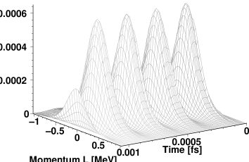
Figure 1: Time and momentum dependence of the distribution function $f({\vec{p}},t)$ for $p_{\perp}=0$ obtained with the conditions described in Set Ia of Table 1. This alternating laser field produces repeated cycles of particle creation and annihilation.

Figure 1 depicts the time evolution of the momentum distribution function for electrons produced under currently anticipated XFEL conditions. This relatively weak alternating field generates repeated cycles of pair creation, with about $1.6\times 10^{5}$ local maxima in one laser pulse. The production rate: $S({\vec{p}},t)=df({\vec{p}},t)/dt$, is clearly time-dependent and vanishes at these local maxima. Therefore an estimation of $S$ at a fixed time, as in Refs. Chen ; Ringwald , is potentially misleading. Under these conditions there is no accumulation of produced particles because creation and annihilation processes are balanced; i.e., all the particles produced have sufficient time to annihilate again before the next cycle of particle creation. Hence the number of particles cannot exceed the value at the first of the repeated maxima.

The situation is markedly different for strong fields, as made plain by Fig. 2, which depicts the time evolution of the number density:

$$n(t)=\int\frac{d^{3}p}{(2\pi)^{3}}f({\vec{p}},t)\,.$$ (6)

When $E=E_{cr}$ the interval between bursts of particle creation is so small that not all the particles can annihilate before the next cycle of particle production begins. Therefore the particles accumulate until almost all momentum states are completely occupied. In this case field-current feedback effects may become important.

Figure 2: Time evolution of the number density for Sets I and II, Table 1. In strong fields, particles accumulate, leading to the almost complete occupation of available momentum states. In weak fields, repeated cycles of particle creation and annihilation occur in tune with the laser frequency: $\Omega_{\rm Ia}=2.0\times 10^{18}\,2\pi s^{-1}$; $\Omega_{\rm Ib}=4.0\times 10^{18}\,2\pi s^{-1}$.

Having calculated the time-dependent number density we can estimate the number of particles produced in the spot volume via vacuum decay. Assuming the diffraction limit on focusing can be reached then $r_{\sigma}=\lambda$, $V_{\sigma}\approx\lambda^{3}$, and the peak particle number is

$$N(t_{>})\approx\lambda^{3}\,n(t_{>})\,,$$ (7)

where $t_{>}$ is the time-location of the peak number density (which is any of the local maxima for XFEL fields). Our results are presented in Table 1. We remark that, following a very different route, Ref. Chen also arrives at a value similar to our Set Ia estimate of $\sim 10^{3}$ particles. Increasing the peak field strength by one order of magnitude increases the produced particle yield by $10^{3}$, as is obvious from Fig. 2.

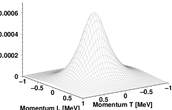
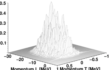
Figure 3: Momentum-dependence of the distribution function: Upper panel, Set Ia; Lower panel Set IIa, Table 1. Note the vastly different magnitudes. The accessible range of longitudinal momenta is magnified for strong fields and the irregular structure expresses the influence of non-Markovian effects in the source term for this case.

Our complete numerical solution also provides the full momentum distribution, which is depicted in Figs. 3. For both weak and strong fields the maximum transverse momentum is approximately $1\,$MeV but the maximum longitudinal momentum is much larger for strong fields. This result owes itself to the minimal coupling of the vector potential to the parallel momentum component but is invisible for weak fields. Furthermore the presence of non-Markovian effects for strong fields (see discussion of Eq. (3)) is evident in the irregular structure in the lower panel cf. the smooth distribution in the XFEL-like field distribution depicted in the upper panel.

In Fig. 4 we plot the time evolution of the current. For an XFEL-like field the induced current is zero on the scale of this figure. (NB. It is a factor of $10^{3}$ smaller than the external current.) The plasma oscillation period in this system can be estimated using the ultrarelativistic formula

$$\tau_{\rm pl}^{UR}\approx\frac{\sqrt{n_{max}m_{e}+E_{cr}^{2}}}{n_{max}e/2}\approx 6.5\times 10^{-19}\,s$$ (8)

cf. the laser periods: $2.5\times 10^{-19}\,$s and $5.0\times 10^{-19}\,$s, which shows that the oscillatory behaviour evident in the figure is prescribed by the laser frequency. (NB. It emphasises, however, that were the amplitude of the induced current larger, field-current feedback may become important.) The behaviour of the strong field current is instructive. The focused laser beams generate a volume of high field strength in which particles are created. The strong field persists long enough for all the particles to be accelerated to their maximum velocity, almost the speed of light in this case, which explains the appearance of the plateaux: the current saturates when all the produced particles reach their terminal velocity. The plateaux end as the alternating laser field changes sign and accelerates the electrons in the opposite direction. Each successive plateau is higher because, as explained in connection with Fig. 2, for strong fields the period between particle production cycles is small and hence there is a net accumulation of particles.

Figure 4: Current for Sets II of Table 1. The plateaux occur when the produced particles reach their terminal velocity, almost the speed of light. The oscillatory behaviour is driven by the laser frequency. (NB. For an XFEL-like field the current is zero on the scale of this figure.)

We have explored the possibility of electron-positron pair production through vacuum decay at the focus of achievable X-ray free electron laser beams via the self-consistent solution of a quantum Vlasov equation coupled to Maxwell’s equation. This is a rigorous application of non-equilibrium quantum mean field theory. Our complete calculation confirms that the effect will be observable if proposed facilities achieve their design goals. Under such conditions the production rate is time-dependent, with repeated cycles of particle production and annihilation in tune with the laser frequency, but the peak particle number is independent of the laser frequency: up to $10^{3}$ pairs may be produced in the spot volume. Our procedure yields the full single particle momentum distribution function (Fig. 3) and hence provides comprehensive phase space information about the $e^{+}e^{-}$ pairs. It also verifies that, at present design goals: collisions among the produced particles can be neglected because the maximum particle number density is low (Fig. 2); a Schwinger-like source term is adequate because the non-Markovian features of the true source term have no impact (Fig. 3) and hence the low density approximation to the distribution function, Eq. (5), is accurate; and field-current feedback will not influence the production process (Fig. 4).

- (1) F. Sauter, Z. Phys. 69, 742 (1931); W. Heisenberg and H. Euler, Z. Phys. 98, 714 (1936); J. Schwinger, Phys. Rev. 82, 664 (1951).
- (2) See, e.g., S. Scherer et al., Prog. Part. Nucl. Phys. 42 (1999) 279.
- (3) C.D. Roberts and S.M. Schmidt, Prog. Part. Nucl. Phys. 45 (2000) S1.
- (4) Y. Kluger et al., Phys. Rev. Lett. 67 (1991) 2427.
- (5) J.C.R. Bloch et al., Phys. Rev. D 60 (1999) 116011.
- (6) A. Bialas et al., Nucl. Phys. B 296, 611 (1988); D.V. Vinnik et al., “Plasma production and thermalisation in a strong field,” nucl-th/0103073.
- (7) E. Brezin and C. Itzykson, Phys. Rev. D 2, 1191 (1970).
- (8) V.S. Popov and M.S. Marinov, Yad. Fiz. 16, 809 (1972) [Sov. J. Nucl. Phys. 16, 449 (1973)]; N.B. Narozhnyi and A.I. Nikishov, Zh. Eksp. Teor. Fiz. 65, 862 (1973) [Sov. Phys. JETP 38, 427 (1974)].
- (9) I. Lindau, M. Cornacchia and J. Arthur, in Workshop On The Development Of Future Linear Electron-Positron Colliders For Particle Physics Studies And For Research Using Free Electron Lasers, eds. G. Jarlskog, U. Mjörnmark and T. Sjöstrand (Lund University, 1999), pp. 153-161.
- (10) TESLA – The Superconductiong Electron Positron Linear Collider with an Integrated X-Ray Laser Laboratory, Technical Design Report, DESY 2001-011, ECFA 2001-209, TESLA-Report 2001-23, TESLA-FEL 2001-05.
- (11) P. Chen and C. Pellegrini, in Quantum Aspects of Beam Physics, Proc. 15th Advanced ICFA Beam Dynamics Workshop, Monterey, Calif., 4-9 Jan 1998, ed. P. Chen (World Scientific, Singapore, 1998) 571.
- (12) A. Ringwald, Phys. Lett. B 510, 107 (2001).
- (13) S.A. Smolyansky et al., hep-ph/9712377; S.M Schmidt et al., Int. J. Mod. Phys. E 7, 209 (1998).
- (14) Y. Kluger, E. Mottola, and J.M. Eisenberg, Phys. Rev. D 58, 125015 (1998).
- (15) J. Rau and B Müller, Phys. Rep. 272, 1 (1996).
- (16) S.M. Schmidt, et al., Phys. Rev. D 59, 094005 (1999); J.C.R. Bloch, C.D. Roberts and S.M. Schmidt, Phys. Rev. D 61, 117502 (2000).
- (17) G.J. Troup and H.S. Perlman, Phys. Rev. D 6, 2299 (1972).