nucl-th/0110006

TUM-T39-01-22

ECT*-01-27

1st October 2001

Re-revised version 13th February 2002, Phys. Rev. C65

Dispersion Effects in Nucleon Polarisabilities

Harald W. Grießhammer and Thomas R. Hemmert

Institut für Theoretische Physik (T39), Physik-Department,
Technische Universität München, D-85747 Garching, Germany

and

ECT*, Villa Tambosi, I-38050 Villazzano (Trento), Italy

We present a formalism to extract the dynamical nucleon polarisabilities defined via a multipole expansion of the structure amplitudes in nucleon Compton scattering. In contradistinction to the static polarisabilities, dynamical polarisabilities gauge the response of the internal degrees of freedom of a composed object to an external, real photon field of arbitrary energy. Being energy dependent, they therefore contain additional information about dispersive effects induced by internal relaxation mechanisms, baryonic resonances and meson production thresholds of the nucleon. We give explicit formulae to extract the dynamical electric and magnetic dipole as well as quadrupole polarisabilities from low energy nucleon Compton scattering up to the one pion production threshold and discuss the connection to the definition of static nucleon polarisabilities. As a concrete example, we examine the results of leading order Heavy Baryon Chiral Perturbation Theory for the four leading spin independent iso-scalar polarisabilities of the nucleon. Finally, we consider the possible rôle of energy dependent effects in low energy extractions of the iso-scalar dipole polarisabilities from Compton scattering on the deuteron.

Suggested PACS numbers: 14.20.Dh, 13.40.-f, 13.60.Fz Suggested Keywords: Effective Field Theory, nucleon polarisabilities, Compton scattering

1 Introduction

The study of the low energy structure of the nucleon via Compton scattering $\gamma N\rightarrow\gamma^{\prime}N$ has a long history. For a proton target, one is tempted to obtain a good description of the resulting cross section up to photon energies of about $50\;\mathrm{MeV}$ by assuming that one scatters off a positively charged point-like spin 1/2 particle with an additional (Pauli) anomalous magnetic moment of $\kappa_{p}=1.79$ nuclear magnetons. For higher photon energies, this simple picture breaks down as more details of the complicated internal structure of the nucleon become visible to the electro-magnetic probe. Even at low energies the description can be improved by noting that there are additional effects due to the target structure which turn out to be nearly as large as the magnetic moment terms. It has been argued (see e.g. [1]) that to first order one can take these effects into account via an effective Hamiltonian ansatz

$$H_{\mathrm{eff}}=-\frac{1}{2}\;4\pi\left(\bar{\alpha}_{E}\;\vec{E}^{2}+\bar{\beta}_{M}\;\vec{B}^{2}\right)\;\;,$$ (1.1)

where $\bar{\alpha}_{E}\;(\bar{\beta}_{M})$ constitutes the electric (magnetic) polarisability of the nucleon in response to an external electric (magnetic) field $\vec{E}\;(\vec{B})$ generated by the incoming and outgoing photon. In the past few decades, a lot of effort has been invested to determine these fundamental structure parameters of the nucleon. The most recent global analysis of the world data for the proton [2] gives

$$\bar{\alpha}_{p} = \left(11.9\pm 0.5\mp 0.5\right)\times 10^{-4}\;\mathrm{fm}^{3}$$

$$\bar{\beta}_{p} = \left(1.5\pm 0.6\pm 0.2\right)\times 10^{-4}\;\mathrm{fm}^{3}\;\;,$$ (1.2)

whereas the neutron polarisabilities are less well determined, with sometimes conflicting experiments, see e.g. recently [3, 4] and references in [5]

$$\bar{\alpha}_{n} = [0\dots 16.6]\times 10^{-4}\;\mathrm{fm}^{3}$$

$$\bar{\beta}_{n} = [1.2\dots 14]\times 10^{-4}\;\mathrm{fm}^{3}\;\;.$$ (1.3)

Here, we do not want to comment on the accuracy, error bars or inherent problems of the neutron measurements. Rather, we want to point out that the numbers displayed in (1/1) attempt to describe the nucleon’s response to a static external electro-magnetic $\vec{E},\,\vec{B}$ field, which in the language of nucleon Compton scattering corresponds to the limit that the energy of the incoming photon goes to zero. Obviously, the experiments from which the numbers of (1) have been derived were not performed at zero energy as there is hardly any sensitivity to the polarisabilities in this kinematic regime. In fact, most of the recent proton Compton scattering experiments were performed with $55$ to $800\;\mathrm{MeV}$ photons [2, 6, 7] and thus had to rely on additional, theoretical input to relate the results to zero energy parameters. In other words, one needs to know the energy dependence of the various nucleon structure parameters in order to extract static nucleon properties. For photon energies below the two pion production threshold, the most convenient way to take these effects into account is the use of dispersion theory. Its starting point is a dispersion relation for each of the six invariant amplitudes governing spin 1/2 Compton scattering. The static polarisabilities defined at zero energy can then be related to a subtraction constant of such a (subtracted) dispersion relation, whereas the energy dependent effects are subsumed into the integral over the photo-absorption cross sections $\gamma N\rightarrow X$. Given that there is enough experimental information on the required inelastic cross sections, one can then calculate differential cross sections for nucleon Compton scattering and finally fit the unknown subtraction constants (namely the polarisabilities) to reproduce the measured Compton cross sections. Details on the use of subtracted and unsubtracted dispersion relations in the analysis of medium energy nucleon Compton scattering can be found in [8, 9]. Here, we only want to remind the reader that even in the usual extraction of the static polarisabilities, the correct treatment of the energy dependent effects is crucial. In the following, we argue that this energy dependence is not just a dirty side-effect to be subsumed into a dispersion integral, but that the effect is interesting in its own right, leading to a better understanding of the degrees of freedom which rule the electric and magnetic properties of the nucleon.

The article is organised as follows: In the next section, we discuss a multipole expansion for the nucleon amplitudes of Compton scattering which also serves as point of reference for a discussion of the energy dependent effects expected in nucleons at the end of the same section. Section 3 shows how to extract the dynamical polarisabilities from given Compton amplitudes. We then exemplify our method by calculating the leading one loop order Heavy Baryon Chiral Perturbation prediction for the electric and magnetic dipole and quadrupole polarisabilities (Sect. 4). Before concluding by summarising and discussing our findings, we give an outlook on possible implications of our results on the extraction of nucleon polarisabilities from Compton scattering off the deuteron in Sect. 5.

2 Multipole Expansion

The $T$ matrix of nucleon Compton scattering can be written in terms of six amplitudes $A_{i}(\omega,z),\;i=1,\dots,6$. In the following, we will work in the centre-of-mass (cm) frame and use the Compton amplitudes of [10]. Thus, $\omega$ denotes the cm energy of a real photon scattering under the cm angle $\theta$ off the nucleon, with $z=\cos\theta$. Polarisabilities are designed to be a measure of the excitation spectrum of a system, but low energy Compton scattering off the proton is dominated by Born terms, i.e. by the successive interactions of two photons with a point-like nucleon with charge Q and anomalous magnetic moment $\kappa$. It is therefore customary to subtract these “nucleon pole” effects from the six Compton amplitudes and only analyse the remainder in terms of polarisabilities. Clearly, the differential cross sections are independent of this artificial separation of the amplitudes into “pole” and “non-pole” parts. Here, we only state the principle

$$\bar{A}_{i}(\omega,z) = A_{i}(\omega,z)-A_{i}^{\mathrm{pole}}(\omega,z),\;i=1,\dots,6$$ (2.1)

with the caveat that any theoretical calculation of nucleon polarisabilities should state carefully which definition of “nucleon pole” terms, which set of Compton amplitudes and – in the case of non-relativistic frameworks – which frame of reference was used. A covariant definition of “nucleon pole” terms can be found e.g. in [1]. In the following, we will only discuss the “non-pole” amplitudes $\bar{A}_{i}$.

The electric and magnetic polarisabilities of the nucleon are contained in the two spin independent structure amplitudes $\bar{A}_{1},\;\bar{A}_{2}$:

$$\bar{T}(\omega,z)= \bar{A}_{1}(\omega,z)\;\vec{\epsilon}^{\prime\,\ast}\cdot\vec{\epsilon}+\bar{A}_{2}(\omega,z)\;\left(\vec{\epsilon}^{\prime\,\ast}\cdot\hat{\vec{k}}\right)\,\left(\vec{\epsilon}\cdot\hat{\vec{k}}{}^{\prime}\right)+\ldots\;\;,$$ (2.2)

where $\hat{\vec{k}}=\vec{k}/\omega$ ($\hat{\vec{k}}{}^{\prime}=\vec{k}^{\prime}/\omega$) is the unit vector in the direction of the momentum of the incoming (outgoing) photon.

A multipole expansion for Compton scattering has been defined a long time ago [12, 13, 14] in a different basis $R_{i}$. With the connecting formula

$$\bar{A}_{1}(\omega,z) = \frac{4\pi\,W}{M}\left[\bar{R}_{1}(\omega,z)+z\,\bar{R}_{2}(\omega,z)\right]$$

$$\bar{A}_{2}(\omega,z) = -\,\frac{4\pi\,W}{M}\,\bar{R}_{2}(\omega,z)\;\;,$$ (2.3)

where $W=\omega+\sqrt{M^{2}+\omega^{2}}$ is the total cm energy and $M$ the nucleon mass, we can easily utilise the known multipole expansion of the structure dependent (“non-pole”) part $\bar{R}_{1},\,\bar{R}_{2}$ of the functions $R_{1},\,R_{2}$ [12, 13, 14]:

$$\bar{R}_{1}(\omega,z) = \sum\limits_{l=1}^{\infty}\Big{\{}\Big{[}(l+1)f_{EE}^{l+}(\omega)+l\,f_{EE}^{l-}(\omega)\Big{]}\Big{(}l\,P_{l}^{\prime}(z)+P_{l-1}^{\prime\prime}(z)\Big{)}-$$

$$\phantom{\sum\limits_{l=1}^{\infty}\Big{\{}}-\Big{[}(l+1)f_{MM}^{l+}(\omega)+l\,f_{MM}^{l-}(\omega)\Big{]}P_{l}^{\prime\prime}(z)\Big{\}}$$

$$\bar{R}_{2}(\omega,z) = \sum\limits_{l=1}^{\infty}\Big{\{}\Big{[}(l+1)f_{MM}^{l+}(\omega)+l\,f_{MM}^{l-}(\omega)\Big{]}\Big{(}l\,P_{l}^{\prime}(z)+P_{l-1}^{\prime\prime}(z)\Big{)}-$$ (2.4)

$$\phantom{\sum\limits_{l=1}^{\infty}\Big{\{}}-\Big{[}(l+1)f_{EE}^{l+}(\omega)+l\,f_{EE}^{l-}(\omega)\Big{]}P_{l}^{\prime\prime}(z)\Big{\}}\;\;,$$

where $P_{i}^{(n)}$ denotes the $n$th derivative of the Legendre polynomial $P_{i}(z)$ with respect to $z$. The multipole amplitudes $f_{TT^{\prime}}^{l\pm}(\omega)$ with $T,T^{\prime}=E,M$ contain the energy dependence and correspond to transitions $Tl\rightarrow T^{\prime}l^{\prime}$, where $l$ corresponds to the angular momentum of the initial photon and $l^{\prime}=l\pm\{1,\,0\}$ to the one of the final photon. The total angular momentum is $l\pm=j=l\pm\frac{1}{2}$. We now define energy dependent electric and magnetic polarisabilities via the relations

$$\alpha_{El}(\omega) = N_{l}\,\frac{l\left(l+1\right)\left[\left(l+1\right)f_{EE}^{l+}+l\,f_{EE}^{l-}\right]}{2\,\omega^{2l}}$$

$$\beta_{Ml}(\omega) = N_{l}\,\frac{l\left(l+1\right)\left[\left(l+1\right)f_{MM}^{l+}+l\,f_{MM}^{l-}\right]}{2\,\omega^{2l}}$$ (2.5)

with $N_{1}=1,\;N_{2}=12,\;N_{l}=\frac{2l}{l+1}\,[(2l-1)!!]^{2}$ being normalisation factors [15] chosen to recover the usual static polarisabilities in the limit of zero photon energy $\omega\rightarrow 0$. For example, the well known static electric and magnetic polarisabilities $\bar{\alpha}_{E},\;\bar{\beta}_{M}$ of the nucleon are recovered as the low energy limit of two electric or magnetic dipole transitions

$$\bar{\alpha}_{E}=\lim_{\omega\rightarrow 0}\alpha_{E1}(\omega)\;\; \bar{\beta}_{M}=\lim_{\omega\rightarrow 0}\beta_{M1}(\omega)\;\;,$$ (2.6)

leading to an excitation of the nucleon and a successive de-excitation with the same multipole character. However, as (2) indicates, there is no need to end the discussion of nucleon structure as tested in Compton scattering at the lowest order of the non-pole level, where only dipole polarisabilities are tested. For example, the static electric and magnetic quadrupole polarisabilities $\bar{\alpha}_{E2},\;\bar{\beta}_{M2}$ originating from the effective Hamiltonian (see e.g. [1])

$$H_{\mathrm{eff}} = -\frac{4\pi}{12}\;\Big{[}\bar{\alpha}_{E2}\;E_{ij}^{2}\;+\;\bar{\beta}_{M2}\;B_{ij}^{2}\Big{]}\;\;,$$ (2.7)

with $T_{ij}:=\frac{1}{2}(\partial_{i}T_{j}+\partial_{j}T_{i}),\;T=E,B$, are recovered via

$$\bar{\alpha}_{E2}=\lim_{\omega\rightarrow 0}\alpha_{E2}(\omega)\;\; \bar{\beta}_{M2}=\lim_{\omega\rightarrow 0}\beta_{M2}(\omega)\;\;.$$ (2.8)

Higher order (static and dynamical) multipoles can be defined at will.

While we follow the definitions of Ref. [1] for the static polarisabilities, we explicitly keep the energy dependence of the dynamical polarisabilities as given via (2). This corresponds to defining the coefficients $\alpha_{El},\;\beta_{Bl}$ in the Hamiltonians (1.1/2.7) as energy dependent, as we demonstrate now.

In the spin independent sector, we can absorb the polarisability-like interactions containing time derivatives of the electric or magnetic field as defined in [1] into the definitions of the dynamical polarisabilities, e.g.

$$-\frac{4\pi}{2}\;\Big{[}\bar{\alpha}_{E}\;\vec{E}^{2}+\bar{\alpha}_{E\nu}\;\dot{\vec{E}^{2}}+\dots\Big{]}\;\to\;-\frac{4\pi}{2}\;\alpha_{E1}(\omega)\;\vec{E}^{2}\;\;.$$ (2.9)

At small enough photon energies, this definition is equivalent to the Taylor expansion of [1],

$$\lim\limits_{\omega\to 0}\alpha_{E1}(\omega)=\bar{\alpha}_{E}+\bar{\alpha}_{E\nu}\;\omega^{2}+\dots\;\;,$$ (2.10)

which clearly has the dis-advantage that the series does not necessarily converge at higher energies. The effective Hamiltonian of the dynamical polarisabilities

$$H_{\mathrm{eff}}^{\mathrm{dyn}}=-4\pi\;\Big{[}\frac{1}{2}\;\Big{(}\alpha_{E1}(\omega)\;\vec{E}^{2}\;+\;\beta_{M1}(\omega)\;\vec{B}^{2}\Big{)}+\frac{1}{12}\;\Big{(}\alpha_{E2}(\omega)\;E_{ij}^{2}\;+\;\beta_{M2}(\omega)\;B_{ij}^{2}\Big{)}\Big{]}\;+\;\dots$$ (2.11)

is thus built only of the spatial multipoles of the photon field, with all temporal response and retardation effects contained in the definition of the dynamical polarisabilities.

We believe that the study of this energy dependence is interesting in its own right as the temporal response of the nucleon to external electro-magnetic perturbations is encoded therein. Recall that polarisabilities are a global measure of the low energy excitation spectrum of a system, and hence mirror the response of the internal degrees of freedom to an external, real photon field. A composite object will therefore necessarily have energy dependent polarisabilities. We also notice that the concept of dispersive effects for the polarisabilities of composite systems is textbook knowledge in classical electro-dynamics and solid state physics. It was also utilised in the Sixties in nuclear structure, mostly in the context of giant dipole resonances of heavy nuclei, see e.g. [18] and references therein.

It is well known from many branches of physics that polarisabilities can become energy dependent due to internal relaxation mechanisms, resonances and particle production thresholds in a physical system. In the first, some of the internal degrees of freedom of the system “freeze out” at some scale as the photon energy is increased because they cannot respond any more to the rapidly varying photon fields. This leads to a drop of the polarisabilities stemming from them as their relaxation time becomes larger than the inverse frequency of the photon field. Resonance effects are traditionally discussed in the Lorentz model which tries to describe their influence on polarisabilities by assuming that the photon field couples to a dampened harmonic multipole oscillator with a proper frequency given by the resonance energy. The width over which the polarisability changes and its maximum are then related to the decay width and strength of the resonance. In the nucleon, we therefore expect explicit $\Delta$, $N^{\ast}$ excitations etc. to make the polarisabilities energy dependent. Finally, production thresholds modify the energy dependence of the polarisabilities, adding above threshold to the dynamical polarisabilities imaginary parts which are necessary to describe the break-up channels not contained in the polarisability Hamiltonian (2.11). The scale over which the polarisabilities vary is in this case set by the mass of the particle produced, and by the strength of the threshold. In the nucleon, the one pion production threshold is the most prominent example. Albeit qualitative in nature, this discussion demonstrates which important information the energy dependence of the polarisabilities contains on the internal degrees of freedom of a system.

We hope to have excited the reader’s imagination about the physics possibilities of studying the energy dependence in dynamical polarisabilities defined via a multipole expansion. We now move on to simple formulae which allow to extract the energy dependence of the leading four spin independent polarisabilities discussed above from any model of nucleon Compton scattering.

3 Matching Formulae

Knowledge of the energy and angular dependence of the pole subtracted structure amplitudes $\bar{A}_{1}(\omega,z)$ and $\bar{A}_{2}(\omega,z)$ in the cm frame as defined in (2.2) suffices to extract the dynamical electric and magnetic dipole and quadrupole polarisabilities of the nucleon. Given these two functions, one has to decide at which angular momentum $l$ to truncate the multipole expansion. Although no requirement of the multipole expansion, we choose to work at energies not higher than the one pion production threshold in Compton scattering to keep the number of multipole polarisabilities small. It is trivial that the higher the photon energy, the more of the higher multipoles have to be included to obtain an accurate result. For any given calculation, it is also simple to check how many multipole polarisabilities defined via (2) have to be included in the expansion until the polarisabilities of interest are stable e.g. at the $5\%$ level. Below, we focus on the first four, $\alpha_{E1}(\omega),\,\beta_{M1}(\omega),\,\alpha_{E2}(\omega)$ and $\beta_{M2}(\omega)$.

The spin independent Compton structure amplitudes $\bar{A}_{1},\;\bar{A}_{2}$ in the cm frame, truncated at $l=3$, read using (2) to (2)

$$\bar{A}_{1}(\omega,z)\Big{|}_{l=3} = \frac{4\pi\,W}{M}\Bigg{[}\Big{(}\alpha_{E1}(\omega)+z\beta_{M1}(\omega)\Big{)}\omega^{2}+\frac{1}{12}\Big{(}z\alpha_{E2}(\omega)+(2z^{2}-1)\beta_{M2}(\omega)\Big{)}\omega^{4}+$$

$$+\;\frac{1}{4N_{3}}\Big{(}(5z^{2}-1)\alpha_{E3}(\omega)+z(15z^{2}-11)\beta_{M3}(\omega)\Big{)}\omega^{6}\Bigg{]}$$

$$\bar{A}_{2}(\omega,z)\Big{|}_{l=3} = -\;\frac{4\pi\,W}{M}\Bigg{[}\beta_{M1}(\omega)\;\omega^{2}+\frac{1}{12}\Big{(}-\alpha_{E2}(\omega)+2z\beta_{M2}(\omega)\Big{)}\omega^{4}+$$ (3.1)

$$+\;\frac{1}{4N_{3}}\Big{(}-10z\alpha_{E3}(\omega)+(15z^{2}-1)\beta_{M3}(\omega)\Big{)}\omega^{6}\Bigg{]}\;\;.$$

Systematically eliminating all dependence on the octupole polarisabilities $\alpha_{E3},\,\beta_{M3}$ and their normalisation factors $N_{3}$ contained in (3), the system of equations for the four leading electric and magnetic dipole and quadrupole polarisabilities in the cm system is easily solved:

$$\alpha_{E1}(\omega)\Big{|}_{l=3} = \frac{M}{4\pi\,W\,\omega^{2}}\;\Big{(}\bar{A}_{1}(\omega,z)\Big{|}_{z=0}-\frac{1}{10}\;\bar{A}_{2}^{\prime}(\omega,z)\Big{|}_{z=0}+\frac{1}{5}\;\bar{A}_{1}^{\prime\prime}(\omega,z)\Big{|}_{z=0}\Big{)}$$

$$\beta_{M1}(\omega)\Big{|}_{l=3} = \frac{M}{8\pi\,W\,\omega^{2}}\;\Big{(}\bar{A}_{1}^{\prime}(\omega,z)\Big{|}_{z=0}-\bar{A}_{2}(\omega,z)\Big{|}_{z=0}-\frac{2}{5}\,\bar{A}_{2}^{\prime\prime}(\omega,z)\Big{|}_{z=0}\Big{)}$$

$$\alpha_{E2}(\omega)\Big{|}_{l=3} = \frac{3M}{2\pi\,W\,\omega^{4}}\;\Big{(}\bar{A}_{1}^{\prime}(\omega,z)\Big{|}_{z=0}+\bar{A}_{2}(\omega,z)\Big{|}_{z=0}-\frac{1}{3}\,\bar{A}_{2}^{\prime\prime}(\omega,z)\Big{|}_{z=0}\Big{)}$$

$$\beta_{M2}(\omega)\Big{|}_{l=3} = \frac{M}{2\pi\,W\,\omega^{4}}\;\Big{(}\bar{A}_{1}^{\prime\prime}(\omega,z)\Big{|}_{z=0}-\bar{A}_{2}^{\prime}(\omega,z)\Big{|}_{z=0}\Big{)}\;,$$ (3.2)

The prime denotes again differentiation with respect to $z=\cos\theta$ in the cm system.

The formulae given in (3) constitute the central result of our investigation. They are valid up to the influence of electro-magnetic $l\geq 4$ transitions and can be applied to any theoretical framework that provides information on the spin independent Compton structure amplitudes $\bar{A}_{1},\,\bar{A}_{2}$. In the example of the iso-scalar nucleon polarisabilities from leading order Heavy Baryon Chiral Perturbation Theory (HB$\chi$PT) discussed in the next section, we will find that effects from $l\geq 4$ can safely be neglected and the formulae given in (3) are by far sufficient to analyse dynamical dipole and quadrupole polarisabilities for photon energies up to the one pion production threshold. We will use this example to demonstrate the feasibility of the kind of studies proposed here. The validity and accuracy of the truncation has of course to be checked separately for each theoretical framework one wants to compare to. This might necessitate to go to $l=4$ or higher for some specific model.

We stress again that the multipole expansion of the Compton amplitudes as performed in (3) is independent of the decision which of the polarisabilities are to be extracted in (3). Of course, wanting to extract the $l_{0}$th multipole polarisabilities, one has to expand the amplitude at least to the $l_{0}$th multipole. However, in that case the $l_{0}$th multipole polarisabilities extracted will also be most sensitive to effects from all the neglected higher multipole polarisabilities $l>l_{0}$. It is therefore prudent to multipole expand (3) to high multipoles $l>l_{0}$, and then limit one in solving the resulting system of equations for the polarisabilities to the first few, $l_{0}$ multipole polarisabilities. As long as the polarisabilities corresponding to higher multipoles are getting smaller and smaller, effects from higher multipoles diminish as $l$ increases.

Finally, we remark that in principle one could also derive our result (3) by utilising projection operators that allow the extraction of individual Compton multipoles $f_{TT^{\prime}}^{l\pm}$ from a set of Compton helicity amplitudes as given by Pfeil et al. [19] and then proceed to reconstruct our definition of dynamical polarisabilities via (2). As we wish to emphasise idea and physical content of the dynamical polarisabilities in this article, we postpone this more formal side to a future publication [11]. Here, it suffices to remark that in the case of the HB$\chi$PT results presented in the next section, we see no change in the quadrupole and dipole polarisabilities when going from $l=2$ to $l=3$ in the expansion of the amplitudes (3). Therefore, the $l=3$ result is in that case for all practical purposes as good as the one obtained from a mathematically rigorous projection formalism.

4 Iso-scalar Nucleon Polarisabilities in Leading Order Heavy Baryon Chiral Perturbation Theory

We now turn as a simple example to the prediction HB$\chi$PT gives at leading one loop order for the dynamical polarisabilities in Compton scattering below the one pion production threshold. We will see that our master formula (3) leads to numerically stable results for the dipole and quadrupole multipoles.

The diagrams contributing to the iso-scalar Compton amplitudes are listed in Fig. 1 [20, 21]. Following the prescription given in [1], we subtract at this order the “nucleon pole” terms

$$A_{1}^{\mathrm{pole}}(\omega)=-\frac{e^{2}}{M}+\mathcal{O}(1/M^{3}) A_{2}^{\mathrm{pole}}(\omega)=\frac{e^{2}\omega}{M^{2}}+\mathcal{O}(1/M^{3})\;\;.$$ , (4.1)

As evident from Fig. 1, the power counting of HB$\chi$PT determines that the leading order contributions to the (dynamical) polarisabilities of the nucleon are generated solely by the surrounding pion cloud. The dynamical polarisabilities will be real functions of $\omega$ as long as the photon energy stays below the pion production threshold. Above the pion production threshold, the polarisabilities will be complex quantities. Following the discussion on the origins of dispersive effects, we therefore expect to see a cusp-like behaviour in the energy dependence as the photon energy approaches $m_{\pi}$. However, we focus the quantitative part of our discussion on Compton scattering below $m_{\pi}$ as we do not expect that the leading order calculation is sufficient to reproduce the correct strength and shape of the energy dependence near the cusp.

Figure 1: The Compton amplitudes $A_{1}$ and $A_{2}$ at leading one loop order in HB$\chi$PT. Graphs obtained by permuting vertices or external lines are not displayed.

Calculating the amplitudes $A_{1},\,A_{2}$ in the cm frame from the diagrams in Fig. 1 to leading one loop order, $\mathcal{O}(p^{3})$, according to [20, 21] and then subtracting the nucleon pole contributions at this order with the help of (4.1), one obtains the Compton structure amplitudes $\bar{A}_{1},\,\bar{A}_{2}$. Inserting them into (3) yields the leading one loop, $\mathcal{O}(p^{3})$, iso-scalar dynamical electric and magnetic dipole and quadrupole polarisabilities in HB$\chi$PT:

$$\alpha_{E1}^{(s)}(\omega)\Big{|}_{l=2} = \frac{{\omega}^{2}}{12}\;\beta_{M2}(\omega)\;+\;\frac{e^{2}g_{A}^{2}}{2\;(4\pi f_{\pi})^{2}}\;\frac{M}{W\omega}\;\int\limits_{0}^{1}\mathrm{d}\!x\;\Bigg{[}a-\sqrt{a^{2}-1}+$$

$$+\;\frac{\left(1+a^{2}\right)}{\sqrt{2}}\;\left(\arctan[\frac{1}{\sqrt{2}a}]-2\arctan[\frac{1-x}{\sqrt{2}{\sqrt{a^{2}-x^{2}}}}]\right)\Bigg{]}$$

$$\beta_{M1}^{(s)}(\omega)\Big{|}_{l=2} = \frac{e^{2}g_{A}^{2}}{16\;(4\pi f_{\pi})^{2}}\;\frac{M}{W\omega}\;\frac{1}{1+2a^{2}}\;\int\limits_{0}^{1}\mathrm{d}\!x\;\Bigg{[}\sqrt{2}\left(2a^{4}-a^{2}-1\right)\arctan[\frac{1}{\sqrt{2}a}]-$$

$$-2\left(a+a^{3}-2\sqrt{2}\left(1+2a^{2}\right)\arctan[\frac{1-x}{\sqrt{2}{\sqrt{a^{2}-x^{2}}}}]\right)\Bigg{]}$$

$$\alpha_{E2}^{(s)}(\omega)\Big{|}_{l=2} = \frac{3e^{2}g_{A}^{2}}{4\;(4\pi f_{\pi})^{2}}\;\frac{M}{W{\omega}^{3}}\;\int\limits_{0}^{1}\mathrm{d}\!x\;\Bigg{[}\sqrt{2}\left(a^{2}-1\right)\arctan[\frac{1}{\sqrt{2}a}]-\;\frac{2a\left(1+a^{2}\right)}{1+2a^{2}}\;-$$

$$-\;\frac{8\left(1+a^{2}\right)\left(x-1\right){\sqrt{a^{2}-x^{2}}}}{1+2a^{2}-x\left(2+x\right)}\;-4\sqrt{2}a^{2}\arctan[\frac{1-x}{\sqrt{2}{\sqrt{a^{2}-x^{2}}}}]\Bigg{]}$$

$$\beta_{M2}^{(s)}(\omega)\Big{|}_{l=3} = \frac{e^{2}g_{A}^{2}}{8\;(4\pi f_{\pi})^{2}}\;\frac{M}{W{\omega}^{3}}\;\int\limits_{0}^{1}\mathrm{d}\!x\;\Bigg{[}-\;\frac{2a\left(1+3{a}^{2}+6{a}^{4}\right)}{{\left(1+2{a}^{2}\right)}^{2}}\;+\;\frac{8\left(x-1\right)\sqrt{a^{2}-x^{2}}}{1+2a^{2}-x\left(2+x\right)}\;+$$

$$\;+\;\sqrt{2}\;\left(\left(3a^{2}-1\right)\arctan[\frac{1}{\sqrt{2}a}]-4\arctan(\frac{x-1}{{\sqrt{2}}{\sqrt{{a}^{2}-x^{2}}}})\right)\Bigg{]}$$

with $f_{\pi}=92\;\mathrm{MeV}$ the pion decay constant and $a:=\frac{m_{\pi}}{\omega}$. The integrals over the Feynman parameter $x$ can be performed by standard methods, but the outcome is not especially enlightening and hence is omitted here.

Recall that iso-scalar quantities are defined as the average of the corresponding proton and neutron values. The (dynamical) iso-vector dipole and quadrupole polarisabilities are identically zero to this order in the chiral calculation and hence are not considered. Notice that we give the expressions for the polarisabilities $\alpha_{E1}^{(s)},\;\alpha_{E2}^{(s)}$ and $\beta_{M1}^{(s)}$ only up to $l=2$, while we choose the truncation at $l=3$ for $\beta_{M2}^{(s)}$ to increase the numerical accuracy as discussed below. To derive the complete result up to $l=3$ is straightforward, but we refrain from quoting it as the expressions are lengthy and the numerical difference between $l=2$ and $l=3$ for $\alpha_{E1}^{(s)},\;\alpha_{E2}^{(s)}$ and $\beta_{M1}^{(s)}$ is tiny. Instead, we plot the dynamical polarisabilities of the $l=3$ truncation in Fig. 2 together with results for $l=1$ and $l=2$ truncations, using the axial nucleon coupling $g_{A}=1.27$ and the iso-scalar masses $m_{\pi}=138\;\mathrm{MeV}$ and $M=939\;\mathrm{MeV}$.

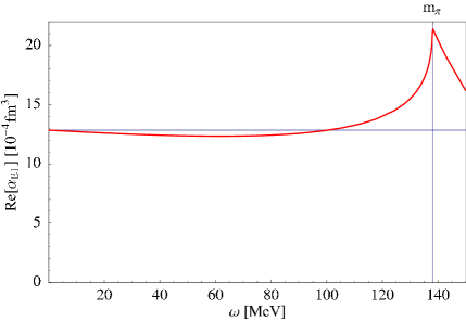
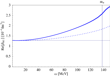
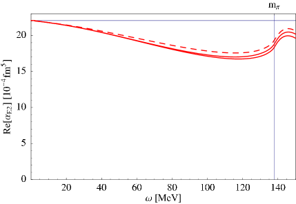
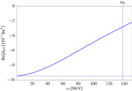
Figure 2: Leading one loop order HB$\chi$PT prediction for the dependence of the dynamical iso-scalar electric and magnetic dipole (top) and quadrupole (bottom) polarisabilities on the photon energy. Solid (dotted; dashed) lines: extraction truncated at $l=3$ ($l=1$; $l=2$). Notice the different scales. The upper left figure shows indeed three lines.

In the limit $\omega\rightarrow 0$, the expressions (4) recover the well-known leading order HB$\chi$PT predictions for the iso-scalar electric and magnetic dipole polarisabilities $\bar{\alpha}_{E}^{(s)},\,\bar{\beta}_{M}^{(s)}$ [20, 21], as well as the predictions for their less known iso-scalar quadrupole counterparts $\bar{\alpha}_{E2}^{(s)},\,\bar{\beta}_{M2}^{(s)}$ [1]. This can easily be checked by Taylor expanding (4) in the photon energy $\omega$:

$$\alpha_{E1}^{(s)}(\omega\to 0) = \frac{5e^{2}g_{A}^{2}}{24\;(4\pi f_{\pi})^{2}\;m_{\pi}}\;\left[\left(1-\frac{\omega}{M}+\frac{\omega^{2}}{2M^{2}}\right)+\frac{9}{100}\;\frac{\omega^{2}}{m_{\pi}^{2}}+\mathcal{O}(\omega^{3})\right]$$

$$\beta_{M1}^{(s)}(\omega\to 0) = \frac{e^{2}g_{A}^{2}}{48\;(4\pi f_{\pi})^{2}\;m_{\pi}}\;\left[\left(1-\frac{\omega}{M}+\frac{\omega^{2}}{2M^{2}}\right)+\frac{7}{5}\;\frac{\omega^{2}}{m_{\pi}^{2}}+\mathcal{O}(\omega^{3})\right]$$

$$\alpha_{E2}^{(s)}(\omega\to 0) = \frac{7e^{2}g_{A}^{2}}{40\;(4\pi f_{\pi})^{2}\;m_{\pi}^{3}}\;\left[\left(1-\frac{\omega}{M}+\frac{\omega^{2}}{2M^{2}}\right)-\frac{521}{1176}\;\frac{\omega^{2}}{m_{\pi}^{2}}+\mathcal{O}(\omega^{3})\right]$$

$$\beta_{M2}^{(s)}(\omega\to 0) = -\frac{3e^{2}g_{A}^{2}}{40\;(4\pi f_{\pi})^{2}\;m_{\pi}^{3}}\;\left[\left(1-\frac{\omega}{M}+\frac{\omega^{2}}{2M^{2}}\right)-\frac{47}{42}\;\frac{\omega^{2}}{m_{\pi}^{2}}+\mathcal{O}(\omega^{3})\right]$$ (4.3)

Note that the Taylor expansion in the photon energy at $\mathcal{O}(p^{3})$ does not correspond to a chiral $1/M$ expansion, but that the intrinsic scale $m_{\pi}$ connected to the structure of the nucleon enters as well. The terms in (4) which explicitly depend on the nucleon mass stem from expanding the kinematical factors $M/W$ in (3/6) and are expected to receive corrections from the next order, $\mathcal{O}(p^{4})$, calculation. We only show (4) to emphasise once more that our dynamical polarisabilities are defined in the cm frame and therefore are not required to be symmetric functions in $\omega$.

The plots in Fig. 2 show that for the four leading spin independent dynamical polarisabilities there is hardly any visible difference between the $l=2$ and $l=3$ truncations of the Compton structure amplitudes as defined in (3), at least in the energy range below the one pion threshold. The most pronounced effects related to the truncation of the multipole series of the amplitude can be found in $\alpha_{E2}^{(s)}$ for $\omega\sim 110\;\mathrm{MeV}$, but even there the effect is on the $5\%$ level. Furthermore, the two formulae for the extraction of $\beta_{M1}(\omega)$ and $\alpha_{E2}(\omega)$ (3/6) can be seen in Fig. 2 to agree at the percent level, justifying the omission of all $l\geq 4$ contributions in the multipole expansion of the amplitudes. We also note that if one is only interested in dynamical dipole polarisabilities, even the $l=2$ truncation seems to suffice. This means that in $\bar{A}_{1}$, one only needs information up to quadratic terms in $\cos\theta$, and in $\bar{A}_{2}$ even only the linear dependence is required for a multipole projection.

We now turn to the physics discussion of each polarisability shown in Fig. 2.

• The surprising find – at least to leading one loop order in HB$\chi$PT– in the dynamical iso-scalar electric dipole polarisability $\alpha_{E1}^{(s)}$ is that out to photon energies of $100\;\mathrm{MeV}$, there is hardly any significant energy dependence. The contribution from the pion cloud produces a large value for $\bar{\alpha}_{E}^{(s)}$ which stays nearly constant throughout the low energy region. The only pronounced energy dependence results from the cusp-effect of the one pion production threshold and is expected following the discussion at the end of Sect. 2. Clearly, this finding has to be checked at the next order in HB$\chi$PT [11]. If the pion cloud contributions then still do not result in a significant energy dependence apart from the expected cusp, any strong deviation from the $\alpha_{E1}^{(s)}(\omega)\approx\bar{\alpha}_{E}$ behaviour found from dispersion analyses could point to degrees of freedom in the nucleon beyond the usual pion nucleon dynamics. Details of this cusp structure are, of course, unlikely to be reproduced correctly by this low order calculation.

• In contrast to $\alpha_{E1}^{(s)}$, the magnetic polarisabilities show large dispersive effects even at moderately low energies: At $\omega=100\;\mathrm{MeV}$, $\beta_{M1}^{(s)}$ is increased by $60\%$. Still, since it is small compared to $\alpha_{E1}^{(s)}$, this increase is small in absolute numbers. The effect of the cusp is again clearly visible in the different slopes above and below the one pion production threshold. At low energies, a relaxation mechanism is clearly at work. We note that the energy dependence in $\beta_{M1}^{(s)}$ is interesting because with its help one might be able to identify the dynamical origin of the rather small overall value for the magnetic dipole polarisability of the proton (1). More speculation on the dynamical content in $\beta_{M1}^{(s)}$ can be found in the concluding section of this presentation.

• The dynamical iso-scalar magnetic quadrupole polarisability $\beta_{M2}^{(s)}$ perhaps shows the most surprising behaviour. At $\omega=100\;\mathrm{MeV}$, it drops to half its static value. Similar to a relaxation effect discussed in Sect. 2, it seems to loose most of its strength in the low energy region. Once more, we emphasise that the only dynamical degrees of freedom contained at this order are connected with the pion cloud of the nucleon. It will be interesting to see whether higher order chiral calculations or dispersion theory can substantiate this disappearance of magnetic quadrupole strength in the nucleon.

• Finally, one observes at low energies a similar albeit less pronounced relaxation behaviour in the dynamical iso-scalar electric quadrupole polarisability $\alpha_{E2}^{(s)}$. However, around $\omega\approx 100\;\mathrm{MeV}$, a second effect of opposite sign connected to the cusp of the one pion threshold is taking over, preventing a sharp falloff in the low energy region. Again, any energy dependence resulting from the electric quadrupole excitation of e.g. the $\Delta$(1232) or other nucleon resonances as an intermediate state are not accounted for at this order in the calculation.

We also note that although $\alpha_{E1}^{(s)}$ is hardly energy dependent at low energies, the dispersive effects in $\beta_{M1}^{(s)}$ can lead to a noticeable increase in the dynamical equivalent of the Baldin sum rule, $\alpha_{E1}^{(s)}(\omega)+\beta_{M1}^{(s)}(\omega)$, from its iso-scalar static value $13.2\times 10^{-4}\;\mathrm{fm}^{3}$.

5 Comments on Compton Scattering off the Deuteron

Before concluding, we briefly dwell on low energy Compton scattering off the deuteron. In contrast to low energy Compton scattering on the proton which is not particularly sensitive to the polarisabilities due to at least equally large effects from the magnetic moment terms, the effects from the nucleon iso-scalar magnetic moments are small in the case of the deuteron, and the sensitivity to polarisability effects is therefore greatly enhanced. As the deuteron is modo grosso an iso-scalar target, the iso-scalar polarisabilities $\alpha_{El}^{(s)}$ and $\beta_{Ml}^{(s)}$ of the previous section are accessed directly.

It has been noticed by various authors, e.g. [3, 4] and [23], that the Compton scattering data on the deuteron taken by the SAL group at $\omega_{\mathrm{Lab}}=95\;\mathrm{MeV}$ [24] seem to prefer a static iso-scalar magnetic dipole polarisability $\bar{\beta}_{M}^{(s)}\approx 7\times 10^{-4}\;\mathrm{fm}^{3}$ which deviates strongly from dispersion analysis predictions and from the proton values, while the static iso-scalar electric dipole polarisability $\bar{\alpha}_{E}^{(s)}\approx 11\times 10^{-4}\;\mathrm{fm}^{3}$ is of the expected size. This leads also to a significant violation of the Baldin sum rule, if the values extracted are taken as the static dipole polarisabilities. In view of the leading order HB$\chi$PT result discussed in the last section, one may speculate these findings to be a sign that the dispersive effects in the iso-scalar single nucleon amplitudes might not be under full control, as the leading order chiral calculation actually hints at a basically unchanged $\alpha_{E1}^{(s)}(\omega)\approx\bar{\alpha}_{E}^{(s)}$ and a rise in $\beta_{M1}^{(s)}(\omega)$ with energy, albeit on a much smaller scale. Partially, such dispersive effects have of course been taken into account in [3, 4]. Likewise, Ref. [23] took the full energy dependence of the leading one loop predictions for the HB$\chi$PT amplitudes $\bar{A}_{1}$ and $\bar{A}_{2}$ as input, together with its prediction $\bar{\beta}_{M1}^{(s)}=1.2\times 10^{-4}\;\mathrm{fm}^{3}$. None of these measures lead to a resolution of the puzzle of the iso-scalar polarisabilities of the nucleon. Clearly, our results given in the previous section cannot provide the solution. However, we emphasise again that large dispersive effects in $\beta_{M1}^{(s)}(\omega)$ could be at the heart of this problem and we believe that the formalism outlined here allows for a systematic study of these effects by comparing state of the art dispersion analyses for nucleon Compton scattering with the best available microscopic calculations of the relevant dynamics in the nucleon. We also note that it might be interesting to re-analyse the SAL data by directly extracting the values of the dynamical polarisabilities following (3/6) in a model independent way. But before one can apply the formalism presented here at the cross section level, one of course first has to provide a similar analysis for the corresponding dynamical spin polarisabilities [11].

Before concluding, we also want to comment on a determination of the iso-scalar dipole polarisabilities of the nucleon from deuteron Compton scattering at very low energies. It was suggested in Ref. [5] that a window exists in the region $\omega\sim 20-50\;\mathrm{MeV}$ in which the nucleon polarisabilities can be extracted in a model independent way without having to know detailed pion dynamics. The authors present a feasibility study with data at $\omega=48\;\mathrm{MeV}$. Dispersive effects were estimated as inducing at most a change on the level of $(\frac{\omega}{m_{\pi}})^{2}\sim 10\%$. The leading one loop order HB$\chi$PT analysis in the last section interestingly also shows that $\alpha_{E1}^{(s)}$ and $\beta_{M1}^{(s)}$ are nearly energy independent in that low energy régime, with changes of less than $10\%$. We thus confirm the authors’ findings that at these low energies, the polarisabilities extracted can be taken as the static ones, and that a two parameter fit of the Compton scattering cross section to $\bar{\alpha}_{E}$ and $\bar{\beta}_{M}$ seems justified. Such a procedure also provides a valuable cross check, as the Baldin sum rule is not used as input.

6 Summary and Outlook

To conclude, we want to encourage the study of the dynamical multipole polarisabilities of the nucleon as an important tool to learn about its internal structure. In contradistinction to the well known static polarisabilities which measure the deformation of an object only in a static electro-magnetic field, the dynamical polarisabilities encountered in many areas of physics gauge the global response to an external, real photon of arbitrary energy. Therefore, they contain additional information about the dispersive effects, i.e. the energy dependence of the polarisabilities, as emphasised in Sect. 2. As they encode the excitation spectrum of the internal degrees of freedom of a composite object in an external electro-magnetic field of definite multipolarity, the nucleon polarisabilities will necessarily be energy dependent due to relaxation effects, resonances and particle production thresholds. Thus, properties of the internal degrees of freedom of the nucleon are directly probed by them.

We defined the dynamical polarisabilities starting from a multipole projection of the nucleon pole subtracted Compton scattering amplitudes and gave explicit formulae how to extract the four leading spin independent multipole polarisabilities (Sect. 3). As a simple example, we considered the predictions of leading one loop order HB$\chi$PT for the dynamical iso-scalar electric and magnetic dipole and quadrupole polarisabilities in Sect. 4. We demonstrated that in this case, truncating the non-pole Compton amplitudes at multipolarity $l=3$ is sufficient to obtain numerically stable and convergent results for the dipole and quadrupole polarisabilities. One of the important results of the chiral calculation is that the energy dependence is likely to be strong for the magnetic polarisabilities even far below the one pion production threshold. This might have consequences for the recent discussions on Compton scattering off the deuteron, as discussed in Sect. 5.

The extension of the formalism to spin polarisabilities is straightforward [11]. In the future, we plan to identify the degrees of freedom relevant for nucleon polarisabilities at low energies by comparing the energy dependence for a set of dynamical nucleon polarisabilities, e.g. calculated in $\mathcal{O}(p^{4})$ $SU(2)$ HB$\chi$PT, with the corresponding curves from dispersion analyses [11]. Finally, we hope that this presentation has reminded the reader that nucleon Compton scattering can provide much more dynamical information on the low energy structure of the nucleon than is contained in the discussion of the usual, static dipole polarisabilities.

References

- [1] D. Babusci, G. Giordano, A. I. L’vov, G. Matone and A. M. Nathan: Phys. Rev. C58, 1013 (1998) [hep-ph/9803347].
- [2] V. Olmos de Leon et al.: Eur. Phys. J. A10, 207 (2001).
- [3] N. R. Kolb et al.: Phys. Rev. Lett. 85, 1388 (2000) [nucl-ex/0003002].
- [4] M. I. Levchuk and A. I. L’vov: Nucl. Phys. A684, 490 (2001) [nucl-th/0010059].
- [5] H. W. Grießhammer and G. Rupak: Phys. Lett. B in print [nucl-th/0012096].
- [6] G. Galler et al.: Phys. Lett. B503, 245 (2001) [nucl-ex/0102003].
- [7] G. Blanpied et al.: Phys. Rev. C64, 025203 (2001).
- [8] A. I. L’vov, V. A. Petrunkin and M. Schumacher: Phys. Rev. C55, 359 (1997).
- [9] D. Drechsel, M. Gorchtein, B. Pasquini and M. Vanderhaeghen: Phys. Rev. C61, 015204 (2000) [hep-ph/0103172].
- [10] see e.g. T. R. Hemmert, B. R. Holstein, J. Kambor and G. Knöchlein: Phys. Rev. D57, 5746 (1998) [nucl-th/9709063] and references therein.
- [11] H. W. Grießhammer, T. R. Hemmert, R. Hildebrandt and B. Pasquinig: in preparation.
- [12] V. I. Ritus: Sov. Phys. JETP 5, 1249 (1957).
- [13] A. P. Contogouris: Nuovo Cimento 25, 104 (1962).
- [14] Y. Nagashima: Prog. Theor. Phys. 33, 828 (1965).
- [15] I. Guiaşu and E. E. Radescu: Ann. Phys. textbf120, 145 (1979).
- [16] P. A. M. Guichon, G. Q. Liu and A. W. Thomas: Nucl. Phys. A591, 606 (1995) [nucl-th/9605031].
- [17] A. I. L’vov, S. Scherer, B. Pasquini, C. Unkmeir and D. Drechsel: Phys. Rev. C64, 015203 (2001) [hep-ph/0103172].
- [18] H. Arenhovel and W. Greiner: Prog. Nucl. Phys. 10, 167 (1969).
- [19] W. Pfeil, H. Rollnik and S. Stankowski: Nucl. Phys. B73, 166 (1974).
- [20] V. Bernard, J. Kambor, N. Kaiser and U.-G. Meißner: Nucl. Phys. B388, 315 (1992).
- [21] V. Bernard, N. Kaiser and U.-G. Meißner: Int. J. Mod. Phys. E4, 193 (1995).
- [22] T. R. Hemmert in “Chiral Dynamics 2000: Theory and Experiment III”, eds. A. M. Bernstein, J. L. Goity and U.-G. Meißner, World Scientific 2001, [nucl-th/0101054].
- [23] S. R. Beane in “Chiral Dynamics 2000: Theory and Experiment III”, eds. A. M. Bernstein, J. L. Goity and U.-G. Meißner, World Scientific 2001, [nucl-th/0012042].
- [24] D. L. Hornidge et al.: Phys. Rev. Lett. 84, 2334 (2000) [nucl-ex/9909015].
- [25] V. Bernard, N. Kaiser, U.-G. Meißner and A. Schmitt: Phys. Lett. B319, 269 (1993) [hep-ph/9309211].