Nonlocality of the $NN$ interaction in an effective field theory

Abstract

We investigate low energy nucleon dynamics in the effective field theory (EFT) of nuclear forces. In leading order of the two-nucleon EFT we show that nucleon dynamics is governed by the generalized dynamical equation with a nonlocal-in-time interaction operator. This equation is shown to open new possibilities for applying the EFT approach to the description of low energy nucleon dynamics.

I Introduction

Understanding how nuclear forces emerge from the fundamental theory of quantum chromodynamics (QCD) is one of the most important problems of quantum physics. To study hadron dynamics at scales where QCD is strongly coupled, it is useful to employ effective field theories (EFT’s) [1,2], invaluable tools for computing physical quantities in the theories with disparate energy scales. Following the early work of Weinberg and others [3-7], the EFT approach has become very popular in nuclear physics [8,9]. A fundamental difficulty in an EFT description of nuclear forces is that effective Lagrangians which are used within its framework yield graphs which are divergent, and give rise to singular quantum-mechanical potentials. These potentials do not satisfy the requirements of ordinary quantum mechanics and need to be regulated, and renormalization must be performed. In this way one can successfully perform calculations of many quantities in nuclear physics. However, in this case one cannot parametrize the interactions of nucleons, by using some Lagrangian or Hamiltonian. In fact, in quantum field theory, knowing the Lagrangian is not sufficient to compute results for physical quantities. In addition, one needs to specify a way to make all infinite quantities finite. Another consequence of this situation is that there are not any equations for renormalized amplitudes in subtractive EFT’s: In order to resolve this problem, in some EFT’s [6,10,11] finite cutoff regularization is used. However, renormalization is required to render such theories consistent, and certain cutoff-dependent terms have to be absorbed into the constants before determining them from empirical data.

If the EFT approach, as it is widely believed, is able to provide a fundamental description of the interactions of nucleons at low energies, one can hope that it will give rise to parametrization of these interactions by interaction operators as fundamental as the Coulomb potential, that parametrizes the interaction of charged particles in low energy QED. In the quantum mechanics of particles interacting via the Coulomb potential, which is an example of the effective theory, one deals with a well-defined interaction Hamiltonian and the Schrödinger equation governing the dynamics of the theory. This theory is self-consistent, and provides an excellent description of atomic phenomena at low energies. In light of this fact one can expect that the EFT of nuclear forces will allow one to construct a well-defined operator parametrizing the interaction of nucleons and governing their dynamics. At the same time, since the EFT leads to singular nucleon potentials, this operator must not be an interaction Hamiltonian. In the present paper we show that recent developments in quantum theory provide the possibility of a consistent description of nucleon dynamics predicted by the EFT approach.

The above problem of subtractive EFT’s is the same that arises in any quantum field theory with UV divergences: Regularization and renormalization allow one to render the physical predictions finite, however, it is impossible to construct a renormalized Hamiltonian acting on the Fock space, i.e., after renormalization the dynamics of the theory is not governed by the Schrödinger equation. This equation is local in time, and the interaction Hamiltonian describes an instantaneous interaction. On the other hand, locality is the main cause of UV divergences in quantum field theory (QFT), and hence regularization and renormalization may be considered as some ways of nonlocalization of the theory. In Ref. [12] it has been shown that the use of the Feynman approach [13] to quantum theory in combination with the canonical approach allows one to extend quantum dynamics to describe the evolution of a system whose dynamics is generated by a nonlocal-in-time interaction, and an equation of motion has been derived as the most general dynamical equation consistent with the current concepts of quantum theory. Being equivalent to the Schrödinger equation in the particular case where interaction is instantaneous, this equation permits the generalization to the case where the interaction operator is nonlocal in time. It has been shown [12] that a generalized quantum dynamics (GQD) developed in this way provides a new insight into the problem of UV divergences.

The aim of the present paper is to show that the formalism of the GQD developed in Ref. [12] opens new possibilities in the effective theory of nuclear forces. We show that in leading order of the two-nucleon EFT nucleon dynamics is governed by the generalized dynamical equation with a nonlocal-in-time interaction operator. By using the example of the $T$ matrix that describes the contact term in leading order, we investigate the dynamical situation in an EFT after renormalization. We show that this $T$ matrix has the properties that are completely unsatisfactory from the point of view of ordinary quantum mechanics, but satisfies the generalized dynamical equation. Moreover, in this case we deal with the dynamics that is described by the model developed in Refs. [12,14] as a test model demonstrating the possibility of the extension of quantum dynamics to the case of nonlocal-in-time interactions. As has been shown [12], there are no physical reasons to restrict ourselves to the case of local interactions where the generalized dynamical equation is equivalent to the Schrödinger equation: The dynamics corresponding to any solution of this equation is not at variance with the current concepts of quantum physics. This means that the situation where the dynamics is generated by nonlocal-in-time interaction is possible in principle. In the present paper we show that this possibility is realized in the case of low energy nucleon dynamics, and in leading order this dynamics is governed by a nonlocal-in-time interaction operator that is considered in the exactly solvable model [12,14]. We will show that this feature of the GQD permits the parametrization of the $NN$ interactions by operators that are as well defined as, for example, the Coulomb potential, and are independent of renormalization schemes. The advantages of the GQD is that it allows one to describe the evolution of nucleon systems in a consistent way by using equations that do not require renormalization. In the present paper this fact will be proved in leading order of the EFT approach.

In Sec. II we review the principal features of the GQD. In Sec. III we consider the exactly solvable model with nonlocal-in-time interaction and its applications to the description of the $NN$ interaction. The dynamics of a quantum system within the EFT is investigated in Sec. IV. We will consider the nucleons as spinless particles at energies much smaller than their mass, their internal excitation energy, and the range of their interaction, and will investigate nucleon dynamics within the EFT approach developed in Ref. [15]. We show that in leading order this dynamics is equivalent to the dynamics of the model [12,14] with a nonlocal-in-time interaction operator. The dynamical situation that arises in an EFT after renormalization is investigated in Sec. V. Finally, in Sec. VI we present some concluding remarks.

II Generalized quantum dynamics

As has been shown in Ref.R.Kh.:1999 , the Schrödinger equation is not the most general dynamical equation consistent with the current concepts of quantum theory. Let us consider these concepts. As is well known, the canonical formalism is founded on the following assumptions: (i) The physical state of a system is represented by a vector (properly by a ray) of a Hilbert space, and (ii) an observable $A$ is represented by a Hermitian hypermaximal operator $\alpha$. The eigenvalues $a_{r}$ of $\alpha$ give the possible values of $A$. An eigenvector $|\varphi_{r}^{(s)}\rangle$ corresponding to the eigenvalue $a_{r}$ represents a state in which $A$ has the value $a_{r}$. If the system is in the state $|\psi\rangle,$ the probability $P_{r}$ of finding the value $a_{r}$ for $A$, when a measurement is performed, is given by

$$P_{r}=\langle\psi|P_{V_{r}}|\psi\rangle=\sum_{s}|\langle\varphi_{r}^{(s)}|\psi\rangle|^{2},$$

where $P_{V_{r}}$ is the projection operator on the eigenmanifold $V_{r}$ corresponding to $a_{r},$ and the sum $\Sigma_{s}$ is taken over a complete orthonormal set ${|\varphi_{r}^{(s)}\rangle}$ ($s=1,2,...$) of $V_{r}.$ The state of the system immediately after the observation is described by the vector $P_{V_{r}}|\psi\rangle.$

In canonical formalism these postulates are used together with the assumption that the time evolution of a state vector is governed by the Schrödinger equation. However, in QFT the Schrödinger equation is only of formal importance because of the UV divergences. Note in this connection that in the Feynman approach Feynman:1948 to quantum theory this equation is not used as a fundamental dynamical equation. As is well known, the main postulate, on which this approach is founded, is as follows: (iii) The probability of an event is the absolute square of a complex number called the probability amplitude. The joint probability amplitude of a time-ordered sequence of events is product of the separate probability amplitudes of each of these events. The probability amplitude of an event which can happen in several different ways is a sum of the probability amplitudes for each of these ways.

The statements of assumption (iii) express the well-known law for the quantum-mechanical probabilities. Within canonical formalism this law is derived as one of the consequences of the theory. However, in the Feynman formulation of quantum theory this law is used as the main postulate of the theory. The Feynman formulation also contains, as its essential idea, the concept of a probability amplitude associated with a completely specified motion or path in space-time. From assumption (iii) it then follows that the probability amplitude of any event is a sum of the probabilities that a particle has a completely specified path in space-time. The contribution from a single path is postulated to be an exponential whose (imaginary) phase is the classical action (in units of $\hbar$) for the path in question. The above constitutes the contents of the second postulate of the Feynman approach to quantum theory. This postulate is not so fundamental as assumption (iii), which directly follows from the analysis of the phenomenon of quantum interference Feynman:1948 . In Ref.R.Kh.:1999 it has been shown that the first postulate of the Feynman approach [assumption (iii)] can be used in combination with the main fundamental postulates of canonical formalism [assumptions (i) and (ii)] without resorting to the second Feynman postulate and the assumption that the dynamics of a quantum system is governed by the Schrödinger equation. Such a use of the main assumptions of quantum theory leads to a more general dynamical equation than the Schrödinger equation.

In a general case the time evolution of a quantum system is described by the evolution equation

$$|\Psi(t)\rangle=U(t,t_{0})|\Psi(t_{0})\rangle,$$

where $U(t,t_{0})$ is the unitary evolution operator,

$$U^{+}(t,t_{0})U(t,t_{0})=U(t,t_{0})U^{+}(t,t_{0})={\bf 1},$$ (1)

with the group property

$$U(t,t^{\prime})U(t^{\prime},t_{0})=U(t,t_{0}),\quad U(t_{0},t_{0})={\bf 1}.$$ (2)

Here we use the interaction picture. According to assumption (iii), the probability amplitude of an event which can happen in several different ways is a sum of contributions from each alternative way. In particular, the amplitude $\langle\psi_{2}|U(t,t_{0})|\psi_{1}\rangle$ can be represented as a sum of contributions from all alternative ways of realization of the corresponding evolution process. Dividing these alternatives into different classes, we can then analyze such a probability amplitude in different ways. For example, subprocesses with definite instants of the beginning and end of the interaction in the system can be considered as such alternatives. In this way the amplitude $\langle\psi_{2}|U(t,t_{0})|\psi_{1}\rangle$ can be written in the form R.Kh.:1999

$$\langle\psi_{2}|U(t,t_{0})|\psi_{1}\rangle=\langle\psi_{2}|\psi_{1}\rangle$$

$$+\int_{t_{0}}^{t}dt_{2}\int_{t_{0}}^{t_{2}}dt_{1}\langle\psi_{2}|\tilde{S}(t_{2},t_{1})|\psi_{1}\rangle,$$ (3)

where $\langle\psi_{2}|\tilde{S}(t_{2},t_{1})|\psi_{1}\rangle$ is the probability amplitude that if at time $t_{1}$ the system was in the state $|\psi_{1}\rangle,$ then the interaction in the system will begin at time $t_{1}$ and will end at time $t_{2},$ and at this time the system will be in the state $|\psi_{2}\rangle$. Note that in general $\tilde{S}(t_{2},t_{1})$ may be only an operator-valued generalized function of $t_{1}$ and $t_{2}$, since only $U(t,t_{0})={\bf 1}+\int^{t}_{t_{0}}dt_{2}\int^{t_{2}}_{t_{0}}dt_{1}\tilde{S}(t_{2},t_{1})$ must be an operator on the Hilbert space. Nevertheless, it is convenient to call $\tilde{S}(t_{2},t_{1})$ an ”operator”, using this word in the generalized sense. In the case of an isolated system the operator $\tilde{S}(t_{2},t_{1})$ can be represented in the form R.Kh.:1999

$$\tilde{S}(t_{2},t_{1})=\exp(iH_{0}t_{2})\tilde{T}(t_{2}-t_{1})\exp(-iH_{0}t_{1}),$$ (4)

with $H_{0}$ being the free Hamiltonian.

As has been shown in Ref.R.Kh.:1999 , for the evolution operator $U(t,t_{0})$ given by Eq. (3) to be unitary for any times $t_{0}$ and $t$, the operator $\tilde{S}(t_{2},t_{1})$ must satisfy the following equation:

$$(t_{2}-t_{1})\tilde{S}(t_{2},t_{1})=\int^{t_{2}}_{t_{1}}dt_{4}\int^{t_{4}}_{t_{1}}dt_{3}$$

$$\times(t_{4}-t_{3})\tilde{S}(t_{2},t_{4})\tilde{S}(t_{3},t_{1}).$$ (5)

This equation allows one to obtain the operators $\tilde{S}(t_{2},t_{1})$ for any $t_{1}$ and $t_{2}$, if the operators $\tilde{S}(t^{\prime}_{2},t^{\prime}_{1})$ corresponding to infinitesimal duration times $\tau=t^{\prime}_{2}-t^{\prime}_{1}$ of interaction are known. It is natural to assume that most of the contribution to the evolution operator in the limit $t_{2}\to t_{1}$ comes from the processes associated with the fundamental interaction in the system under study. Denoting this contribution by $H_{int}(t_{2},t_{1})$, we can write

$$\tilde{S}(t_{2},t_{1})\mathop{\to}\limits_{t_{2}\rightarrow t_{1}}H_{int}(t_{2},t_{1})+o(\tau^{\epsilon}),$$ (6)

where $\tau=t_{2}-t_{1}$. The parameter $\varepsilon$ is determined by demanding that $H_{int}(t_{2},t_{1})$ must be so close to the solution of Eq. (5) in the limit $t_{2}\mathop{\to}t_{1}$ that this equation has a unique solution having the behavior (6) near the point $t_{2}=t_{1}$. Thus this operator must satisfy the condition

$$(t_{2}-t_{1})H_{int}(t_{2},t_{1})\mathop{\to}\limits_{t_{2}\mathop{\to}t_{1}}\int^{t_{2}}_{t_{1}}dt_{4}\int^{t_{4}}_{t_{1}}dt_{3}(t_{4}-t_{3})$$

$$\times H_{int}(t_{2},t_{4})H_{int}(t_{3},t_{1})+o(\tau^{\epsilon+1}).$$ (7)

Note that the value of the parameter $\epsilon$ depends on the form of the operator $H_{int}(t_{2},t_{1}).$ Since $\tilde{S}(t_{2},t_{1})$ and $H_{int}(t_{2},t_{1})$ are only operator-valued distributions, the mathematical meaning of the conditions (6) and (7) needs to be clarified. We will assume that condition (6) means that

$$\langle\Psi_{2}|\int^{t}_{t_{0}}dt_{2}\int^{t_{2}}_{t_{0}}dt_{1}\tilde{S}(t_{2},t_{1})|\Psi_{1}\rangle$$

$$\mathop{\to}\limits_{t\mathop{\to}t_{0}}\langle\Psi_{2}|\int^{t}_{t_{0}}dt_{2}\int^{t_{2}}_{t_{0}}dt_{1}H_{int}(t_{2},t_{1})|\Psi_{1}\rangle+o(\tau^{\epsilon+2}),$$

for any vectors $|\Psi_{1}\rangle$ and $|\Psi_{2}\rangle$ of the Hilbert space. Condition (7) has to be considered in the same sense.

Within GQD the operator $H_{int}(t_{2},t_{1})$ plays the role the interaction Hamiltonian plays in the ordinary formulation of quantum theory: It generates the dynamics of a system. Being a generalization of the interaction Hamiltonian, this operator is called the generalized interaction operator. If $H_{int}(t_{2},t_{1})$ is specified, Eq. (5) allows one to find the operator $\tilde{S}(t_{2},t_{1}).$ Formula (3) can then be used to construct the evolution operator $U(t,t_{0})$ and accordingly the state vector,

$$|\psi(t)\rangle=|\psi(t_{0})\rangle+\int_{t_{0}}^{t}dt_{2}\int_{t_{0}}^{t_{2}}dt_{1}\tilde{S}(t_{2},t_{1})|\psi(t_{0})\rangle,$$ (8)

at any time $t.$ Thus Eq. (5) can be regarded as an equation of motion for states of a quantum system. By using Eqs. (3) and (4), the evolution operator can be represented in the form

$$\langle n_{2}|U(t,t_{0})|n_{1}\rangle=\langle n_{2}|n_{1}\rangle+\frac{i}{2\pi}\int^{\infty}_{-\infty}dx$$

$$\times\frac{\exp[-i(z-E_{n_{2}})t]\exp[i(z-E_{n_{1}})t_{0}]}{(z-E_{n_{2}})(z-E_{n_{1}})}$$

$$\times\langle n_{2}|T(z)|n_{1}\rangle,$$ (9)

where $z=x+iy$, $y\rangle 0$, and

$$\langle n_{2}|T(z)|n_{1}\rangle=i\int_{0}^{\infty}d\tau\exp(iz\tau)\langle n_{2}|\tilde{T}(\tau)|n_{1}\rangle.$$ (10)

From Eq. (II), for the evolution operator in the Schrödinger picture, we get

$$U_{s}(t,0)=\frac{i}{2\pi}\int^{\infty}_{-\infty}dx\exp(-izt)G(z),$$ (11)

where

$$\langle n_{2}|G(z)|n_{1}\rangle=\frac{\langle n_{2}|n_{1}\rangle}{z-E_{n_{1}}}+\frac{\langle n_{2}|T(z)|n_{1}\rangle}{(z-E_{n_{2}})(z-E_{n_{1}})}.$$ (12)

Eq. (11) is the well-known expression establishing the connection between the evolution operator and the Green operator $G(z)$, and can be regarded as the definition of the operator $G(z)$.

The equation of motion (5) is equivalent to the following equation for the $T$ matrix R.Kh.:1999 :

$$\frac{d\langle n_{2}|T(z)|n_{1}\rangle}{dz}\\ =-\sum\limits_{n}\frac{\langle n_{2}|T(z)|n\rangle\langle n|T(z)|n_{1}\rangle}{(z-E_{n})^{2}},$$

with the boundary condition

$$\langle n_{2}|T(z)|n_{1}\rangle\mathop{\to}\limits_{|z|\mathop{\to}\infty}\langle n_{2}|B(z)|n_{1}\rangle+o(|z|^{-\beta}),$$ (13)

where

$$B(z)=i\int_{0}^{\infty}d\tau\exp(iz\tau)H^{(s)}_{int}(\tau),$$

$\beta=1+\epsilon,$ and

$$H^{(s)}_{int}(t_{2}-t_{1})=\exp(-iH_{0}t_{2})H_{int}(t_{2},t_{1})\exp(iH_{0}t_{1})$$

is the generalized interaction operator in the Schrödinger picture. The solution of Eq. (II) satisfies the equation

$$\langle n_{2}|T(z_{1})|n_{1}\rangle-\langle n_{2}|T(z_{2})|n_{1}\rangle$$

$$=(z_{2}-z_{1})\sum_{n}\frac{\langle n_{2}|T(z_{2})|n\rangle\langle n|T(z_{1})|n_{1}\rangle}{(z_{2}-E_{n})(z_{1}-E_{n})}.$$ (14)

This equation in turn is equivalent to the following equation for the Green operator:

$$G(z_{1})-G(z_{2})=(z_{2}-z_{1})G(z_{2})G(z_{1}).$$ (15)

This is the Hilbert identity, which in the Hamiltonian formalism follows from the fact that in this case the evolution operator (11) satisfies the Schrödinger equation, and hence the Green operator is of the form

$$G(z)=(z-H)^{-1},$$ (16)

with $H$ being the total Hamiltonian. At the same time, as has been shown in Ref.R.Kh.:1999 , Eq. (5) and hence Eqs. (II) and (14) are unique consequences of the unitarity condition and the representation Eq. (3), expressing the Feynman superposition principle [assumption (iii)]. It should be noted that the evolution operator constructed by using the Schrödinger equation can be represented [16] in the form (3). Being written in terms of the operators $\tilde{S}(t_{2},t_{1})$, Eq. (5) does not contain operators describing interaction in the system. It is a relation for $\tilde{S}(t_{2},t_{1})$, which are the contributions to the evolution operator from the processes with defined instants of the beginning and end of the interaction in the systems. Correspondingly, Eqs. (II) and (14) are relations for the $T$ matrix. A remarkable feature of Eq. (5) is that it works as a recurrence relation, and to construct the evolution operator it is sufficient to know the contributions to this operator from the processes with infinitesimal duration times of interaction, i.e. from the processes of a fundamental interaction in the system. This makes it possible to use Eq. (5) as a dynamical equation. Its form does not depend on the specific feature of the interaction (the Schrödinger equation, for example, contains the interaction Hamiltonian). Since Eq. (5) must be satisfied in all the cases, it can be considered as the most general dynamical equation consistent with the current concepts of quantum theory. All the needed dynamical information is contained in the boundary condition for this equation, i.e., in the generalized interaction operator $H_{int}(t_{2},t_{1})$. As has been shown in Ref. R.Kh.:1999 , the dynamics governed by Eq. (5) is equivalent to the Hamiltonian dynamics in the case where the operator $H_{int}(t_{2},t_{1})$ is of the form

$$H_{int}(t_{2},t_{1})=-2i\delta(t_{2}-t_{1})H_{I}(t_{1}),$$ (17)

with $H_{I}(t_{1})$ being the interaction Hamiltonian in the interaction picture. In this case the state vector $|\psi(t)\rangle$ given by Eq. (8) satisfies the Schrödinger equation,

$$\frac{d|\psi(t)\rangle}{dt}=-iH_{I}(t)|\psi(t)\rangle.$$

The delta function $\delta(\tau)$ in Eq. (17) emphasizes that in this case the fundamental interaction is instantaneous. Thus the Schrödinger equation results from the generalized equation of motion (5) in the case where the interaction generating the dynamics of a quantum system is instantaneous. At the same time, Eq. (5) permits the generalization to the case where the interaction generating the dynamics of a quantum system is nonlocal in time R.Kh.:1999 ; R.Kh./A.A.:1999 . In a general case, the generalized interaction operator has the following form R.Kh./A.A.:1999 :

$$H_{int}(t_{2},t_{1})=-2i\delta(t_{2}-t_{1})H_{I}(t_{1})+H_{non}(t_{2},t_{1}),$$

where the first term on the right-hand side of this equation describes the instantaneous component of the interaction generating the dynamics of a quantum system, while the term $H_{non}(t_{2},t_{1})$ represents its nonlocal-in-time part. As has been shown, there is one-to-one correspondence between nonlocality of interaction and the UV behavior of the matrix elements of the evolution operator as a function of momenta of particles: The interaction operator can be nonlocal in time only in the case where this behavior is ”bad”, i.e., in a local theory it results in UV divergences. In Ref. R.Kh.:2001 it has been shown that after renormalization the dynamics of the three-dimensional theory of a neutral scalar field interacting through a $\varphi^{4}$ coupling is governed by the generalized dynamical Eq. (5) with a nonlocal-in-time interaction operator. This lets us expect that after renormalization the dynamics of an EFT is also governed by this equation with a nonlocal interaction operator. In the next section we will consider this problem by using a toy model of the separable $NN$ interaction.

III Models with nonlocal-in-time interactions and the short-range $NN$ interaction

Let us consider the evolution problem for two nonrelativistic particles in the center-of-mass. We denote the relative momentum by ${\bf p}$ and the nucleon mass by $m$. Assume that the generalized interaction operator in the Schrödinger picture $H^{(s)}_{int}(\tau)$ has the form

$$\langle{\bf p}_{2}|H^{(s)}_{int}(\tau)|{\bf p}_{1}\rangle=\varphi^{*}({\bf p}_{2})\varphi({\bf p}_{1})f(\tau),$$

where $f(\tau)$ is some function of $\tau,$ and the form factor $\varphi({\bf p})$ has the following asymptotic behavior for $|{\bf p}|\mathop{\to}\infty:$

$$\varphi({\bf p})\sim|{\bf p}|^{-\alpha},\quad{(|{\bf p}|\mathop{\to}\infty).}$$ (18)

Let, for example, $\varphi({\bf p})$ be of the form

$$\varphi({\bf p})=|{\bf p}|^{-\alpha}+g({\bf{p}}),$$

and in the limit $|{\bf p}|\mathop{\to}\infty$ the function $g({\bf{p}})$ satisfies the estimate $g({\bf{p}})=o(|{\bf{p}}|^{-\delta})$, where $\delta>\alpha,$ $\delta>\frac{3}{2}.$ In the separable case, $\langle{\bf p}_{2}|\tilde{S}(t_{2},t_{1})|{\bf p}_{1}\rangle$ can be represented in the form

$$\langle{\bf p}_{2}|\tilde{S}(t_{2},t_{1})|{\bf p}_{1}\rangle=\varphi^{*}({\bf p}_{2})\varphi({\bf p}_{1})\tilde{s}(t_{2},t_{1}).$$

Correspondingly, $\langle{\bf p}_{2}|T(z)|{\bf p}_{1}\rangle$ is of the form

$$\langle{\bf p}_{2}|T(z)|{\bf p}_{1}\rangle=\varphi^{*}({\bf p}_{2})\varphi({\bf p}_{1})t(z),$$ (19)

where, as it follows from Eq. (II), the function $t(z)$ satisfies the equation

$$\frac{dt(z)}{dz}=-t^{2}(z)\int\frac{d^{3}k}{(2\pi)^{3}}\frac{|\varphi({\bf k})|^{2}}{(z-E_{k})^{2}}$$ (20)

with the asymptotic condition

$$t(z)\mathop{\to}\limits_{|z|\mathop{\to}\infty}f_{1}(z)+o(|z|^{-\beta}),$$ (21)

where

$$f_{1}(z)=i\int_{0}^{\infty}d\tau\exp(iz\tau)f(\tau),$$ (22)

and $E_{k}=\frac{k^{2}}{2\mu}$. The solution of Eq. (20) with the initial condition $t(a)=g_{a},$ where $a\in(-\infty,0),$ is

$$t(z)\\ =g_{a}\left(1+(z-a)g_{a}\int\frac{d^{3}k}{(2\pi)^{3}}\frac{|\varphi({\bf k})|^{2}}{(z-E_{k})(a-E_{k})}\right)^{-1}.$$

In the case $\alpha>\frac{1}{2}$, the function $t(z)$ tends to a constant as $|z|\mathop{\to}\infty$:

$$t(z)\mathop{\to}\limits_{|z|\mathop{\to}\infty}\lambda.$$ (23)

Thus in this case the function $f_{1}(z)$ must also tend to $\lambda$ as $|z|\mathop{\to}\infty.$ From this it follows that the only possible form of the function $f(\tau)$ is

$$f(\tau)=-2i\lambda\delta(\tau)+f^{\prime}(\tau),$$

where the function $f^{\prime}(\tau)$ has no such a singularity at the point $\tau=0$ as does the delta function. In this case the generalized interaction operator $H^{(s)}_{int}(\tau)$ has the form

$$\langle{\bf p}_{2}|H^{(s)}_{int}(\tau)|{\bf p}_{1}\rangle=-2i\lambda\delta(\tau)\varphi^{*}({\bf p}_{2})\varphi({\bf p}_{1}),$$ (24)

and hence the dynamics generated by this operator is equivalent to the dynamics governed by the Schrödinger equation with the separable potential

$$\langle{\bf p}_{2}|H_{I}|{\bf p}_{1}\rangle=\lambda\varphi^{*}({\bf p}_{2})\varphi({\bf p}_{1}).$$ (25)

Solving Eq. (20) with the boundary condition (23), we easily get the well-known expression for the $T$ matrix in the separable-potential model

$$\langle{\bf p}_{2}|T(z)|{\bf p}_{1}\rangle\\ =\varphi^{*}({\bf p}_{2})\varphi({\bf p}_{1})\left(\frac{1}{\lambda}-\int\frac{d^{3}k}{(2\pi)^{3}}\frac{|\varphi({\bf k})|^{2}}{z-E_{k}}\right)^{-1}.$$

Ordinary quantum mechanics does not permit the extension of the above model to the case $\alpha\leq\frac{1}{2}.$ Indeed, in the case of such a large-momentum behavior of the form factors $\varphi({\bf p}),$ the use of the interaction Hamiltonian given by Eq. (25) leads to the UV divergences, i.e., the integral in (III) is not convergent. We will now show that the generalized dynamical Eq. (5) allows one to extend this model to the case $-\frac{1}{2}<\alpha\leq\frac{1}{2}.$ Let us determine the class of the functions $f_{1}(z)$ and correspondingly the value of $\beta$ for which Eq. (20) has a unique solution having the asymptotic behavior (21). In the case $\alpha<\frac{1}{2},$ the function $t(z)$ given by (III) has the following behavior for $|z|\mathop{\to}\infty:$

$$t(z)\mathop{\to}\limits_{|z|\mathop{\to}\infty}b_{1}(-z)^{\alpha-\frac{1}{2}}+b_{2}(-z)^{2\alpha-1}+o(|z|^{2\alpha-1}),$$ (26)

where $b_{1}=-4\pi\cos(\alpha\pi)m^{\alpha-\frac{3}{2}}$ and $b_{2}=b_{1}|a|^{\frac{1}{2}-\alpha}-b_{1}^{2}[M(a)+g_{a}^{-1}]$ with

$$M(a)=\int\frac{d^{3}k}{(2\pi)^{3}}\frac{|\varphi({\bf k})|^{2}-|{\bf{k}}|^{-2\alpha}}{a-E_{k}}.$$

The parameter $b_{1}$ does not depend on $g_{a}.$ This means that all solutions of Eq. (20) have the same leading term in Eq. (29), and only the second term distinguishes the different solutions of this equation. Thus, in order to obtain a unique solution of Eq. (20), we must specify the first two terms in the asymptotic behavior of $t(z)$ for $|z|\mathop{\to}\infty.$ From this it follows that the functions $f_{1}(z)$ must be of the form

$$f_{1}(z)=b_{1}(-z)^{\alpha-\frac{1}{2}}+b_{2}(-z)^{2\alpha-1},$$

and $\beta=1-2\alpha.$ Correspondingly, the functions $f(\tau)$ must be of the form

$$f(\tau)=a_{1}\tau^{-\alpha-\frac{1}{2}}+a_{2}\tau^{-2\alpha},$$ (27)

with $a_{1}=-ib_{1}\Gamma^{-1}(\frac{1}{2}-\alpha)\exp[i(-\frac{\alpha}{2}+\frac{1}{4})\pi],$ and $a_{2}=b_{2}\Gamma^{-1}(1-2\alpha)\exp(-i\alpha\pi),$ where $\Gamma(z)$ is the gamma function. This means that in the case $\alpha<\frac{1}{2}$ the generalized interaction operator must be of the form

$$\langle{\bf p}_{2}|{H}^{(s)}_{int}(\tau)|{\bf p}_{1}\rangle=\varphi^{*}({\bf p}_{2})\varphi({\bf p}_{1})$$

$$\times\left(a_{1}\tau^{-\alpha-\frac{1}{2}}+a_{2}\tau^{-2\alpha}\right),$$ (28)

and, as it follows from Eqs. (19) and (24), for the $T$ matrix we have

$$\langle{\bf p}_{2}|T(z)|{\bf p}_{1}\rangle=N(z)\varphi^{*}({\bf p}_{2})\varphi({\bf p}_{1}),$$ (29)

with

$$N(z)=g_{a}\left(1+(z-a)g_{a}\int\frac{d^{3}k}{(2\pi)^{3}}\frac{|\varphi({\bf k})|^{2}}{(z-E_{k})(a-E_{k})}\right)^{-1},$$

where

$$g_{a}=b_{1}^{2}\left(b_{1}|a|^{\frac{1}{2}-\alpha}-b_{2}-b_{1}^{2}M(a)\right)^{-1}.$$

It can be easily checked that $N(z)$ can be represented in the following form

$$N(z)=\frac{b_{1}^{2}}{-b_{2}+b_{1}(-z)^{\frac{1}{2}-\alpha}+M(z)b_{1}^{2}}.$$

By using Eqs. (II) and (29), we can construct the evolution operator

$$\langle{\bf p}_{2}|U(t,t_{0})|{\bf p}_{1}\rangle=\langle{\bf p}_{2}|{\bf p}_{1}\rangle+\frac{i}{2\pi}\int_{-\infty}^{\infty}dx$$

$$\times\frac{\exp[-i(z-E_{p_{2}})t]\exp[i(z-E_{p_{1}})t_{0}]}{(z-E_{p_{2}})(z-E_{p_{1}})}$$

$$\times\varphi^{*}({\bf p}_{2})\varphi({\bf p}_{1})N(z),$$ (30)

where $z=x+iy,$ and $y>0.$ The evolution operator $U(t,t_{0})$ defined by Eq. (30) is a unitary operator satisfying the composition law (2), provided that the parameter $b_{2}$ is real.

In the case $\alpha=\frac{1}{2}$ the generalized interaction operator must be of the form [17]

$$\langle{\bf p}_{2}|{H}^{(s)}_{int}(\tau)|{\bf p}_{1}\rangle=-\frac{i}{2\pi}\varphi^{*}({\bf p}_{2})\varphi({\bf p}_{1})$$

$$\times\int_{-\infty}^{\infty}dx\exp(-iz\tau)\left(\frac{b_{1}}{\ln(-z)}+\frac{b_{2}}{\ln^{2}(-z)}\right),$$ (31)

where $b_{1}=-\frac{4\pi^{2}}{m}$.

In Ref. R.Kh./A.A.:1999 the model for $\alpha<\frac{1}{2}$ was used for describing the $NN$ interaction at low energies. The motivation to use such a model for parametrization of the $NN$ forces is the fact that due to the quark and gluon degrees of freedom the $NN$ interaction must be nonlocal in time. However, because of the separation of scales the system of hadrons should be regarded as a closed system, i.e., the evolution operator must be unitary and satisfy the composition law. From this it follows that the dynamics of such a system is governed by Eq. (5) with a nonlocal-in-time interaction operator. Let us now parametrize the $NN$ interaction by the generalized interaction operator of the form Eq. (31) with the following form factor:

$$\varphi({\bf p})=\chi({\bf p})+c_{1}g_{Y}({\bf p}),$$

with

$$\chi({\bf p})=\left(d^{2}+p^{2}\right)^{-\frac{\alpha}{2}},\quad-\frac{1}{2}<\alpha<\frac{1}{2},$$

with $g_{Y}({\bf p})$ being the Yamaguchi form factor,

$$g_{Y}({\bf p})=\frac{1}{\beta^{2}+p^{2}}.$$

Here $d,$ $c_{1}$, and $\beta$ are some constants. As it is the generalization of the Yamaguchi model Yam to the case where the $NN$ interaction is nonlocal in time, our model yields the $NN$ phase shifts in good agreement with experiment (see Figs.1-3). The parameters of the model are quoted in Table I. However, the main advantage of this model is that it allows one to investigate the effects of the retardation in the $NN$ interaction caused by the existence of the quark and gluon degrees of freedom on nucleon dynamics.

Table 1: The parameters of the interaction operator obtained by fitting the $NN$ data, $\rho=1{\text{M}eV}^{-1}$.

partial wave	$\alpha$	$c_{1}$	$\beta\times\rho$	$d\times\rho$	$b_{2}\times\rho^{1-2\alpha}$
${}^{3}S_{1}(np)$	0.499	$133.5\times 10^{2}$	433.8	$766.2$	$4.207\times 10^{-5}$
${}^{1}S_{0}(np)$	0.499	131.8	356.3	$3.651\times 10^{6}$	$4.202\times 10^{-5}$
${}^{1}S_{0}(pp)$	0.499	320.0	371.7	$6.763\times 10^{5}$	$4.204\times 10^{-5}$

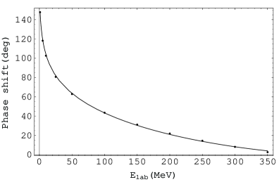
Figure 1: Phase shifts (solid line) in the ${}^{3}S_{1}$ channel for $np$ scattering, compared to the experimental data (points) (Ref. Stoks:1993 ).

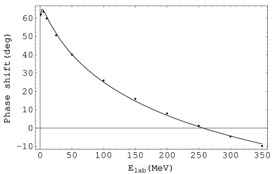
Figure 2: Phase shifts (solid line) in the ${}^{1}S_{0}$ channel for $np$ scattering, compared to the experimental data (points) (Ref. Stoks:1993 ).

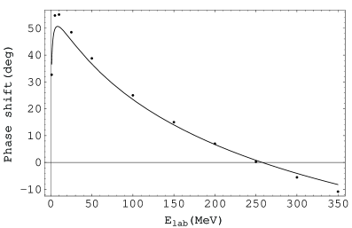
Figure 3: Phase shifts (solid line) in the ${}^{1}S_{0}$ channel for $pp$ scattering, compared to the experimental data (points) (Ref. Stoks:1993 ).

As we have seen, there is the one-to-one correspondence between the form of the generalized interaction operator and the UV behavior of the form factor $\varphi({\bf p}).$ In the case $\alpha>\frac{1}{2},$ the operator $H^{(s)}_{int}(\tau)$ must necessarily have the form (24). In this case the fundamental interaction is instantaneous. In the case $-\frac{1}{2}<\alpha<\frac{1}{2}$ [the restriction $\alpha>-\frac{1}{2}$ is necessary for the integral in Eq. (III) to be convergent], the only possible form of $H^{(s)}_{int}(\tau)$ is Eq. (28), and, in the case $\alpha=\frac{1}{2}$, it must be of the form (31), and hence the interaction generating the dynamics of the system is nonlocal in time. Thus the interaction generating the dynamics can be nonlocal in time only if the form factors have the ”bad” large-momentum behavior that within Hamiltonian dynamics gives rise to the ultraviolet divergences:

$$\text{locality}\quad\Leftrightarrow\varphi({\bf p})\quad\sim\quad|{\bf p}|^{-\alpha},\quad\alpha>\frac{1}{2},$$

$$\text{nonlocality}\Leftrightarrow\varphi({\bf p})\quad\sim\quad|{\bf p}|^{-\alpha},\quad\alpha\leq\frac{1}{2}.$$

From this it follows that the quark-gluon retardation effects must result in the ”bad” UV behavior of the matrix elements of the evolution operator as a function of momenta of hadrons. Note that EFT’s lead to the same conclusion: Within the EFT approach the quark and gluon degrees of freedom manifest themselves in the form of Lagrangians consistent with the symmetries of QCD which gives rise to the UV divergences. Note also that EFT’s are local theories, despite the existence of the external quark and gluon degrees of freedom. However, renormalization of EFT’s gives rise to the fact that these theories become nonlocal.

IV The EFT approach and the nonlocality in time of effective interactions

Let us now investigate the character of the dynamics generated by the two-nucleon EFT. For the sake of simplicity we will restrict ourselves to the model in which the nucleons are considered as spinless. Within the EFT approach the nucleons are considered as particles (described by a field $\Psi$) with three-momenta $Q$ much smaller than their mass $m$, the mass difference $\Delta$ to their first excited state, and the pion mass. If momenta are also small compared to the range of interaction, the $NN$ interaction can be approximated by a sequence of contact interactions, with an increasing number of derivatives. Restricting to parity and time-reversal theories the effective Lagrangian can be written as [15]

$${\cal L}=\Psi^{+}\left(i\partial_{0}+\frac{1}{2m}\nabla^{2}+\frac{1}{8m^{3}}\nabla^{4}+\ldots\right)\Psi$$

$$-\frac{1}{2}C_{0}\Psi^{+}\Psi\Psi^{+}\Psi-\frac{1}{8}(C_{2}+C_{2}^{\prime})\{\Psi^{+}(\overrightarrow{\nabla}$$

$$-\overleftarrow{\nabla})\Psi\cdot\Psi^{+}\left(\overrightarrow{\nabla}-\overleftarrow{\nabla}\right)\Psi-\Psi^{+}\Psi\Psi^{+}\left(\overrightarrow{\nabla}-\overleftarrow{\nabla}\right)^{2}\Psi\}$$

$$+\frac{1}{8}(C_{2}-C_{2}^{\prime})\Psi^{+}\Psi\nabla^{2}(\Psi^{+}\Psi)+\ldots,$$ (32)

where $C_{2n}^{\prime}$s are parameters that depend on the details of the dynamics of range $\sim\frac{1}{m}$. The particles $\Psi$ are nonrelativistic, and evolve only forward in time. Particles number is also conserved. Canonical quantization leads to familiar Feynman rules, and the $\Psi$ propagator at four-momenta $p$ is given by

$$S(p^{0},{\bf p})=\frac{i}{p^{0}-\frac{{\bf p}^{2}}{2m}+\frac{{\bf p}^{4}}{8m^{3}}+\ldots+i\varepsilon}.$$ (33)

The four-$\Psi$ contact interaction is given by $-iv(p,p^{\prime})$, with

$$v(p,p^{\prime})=C_{0}+C_{2}({\bf p}^{2}+{\bf p^{\prime}}^{2})+2C_{2}^{\prime}{\bf p}\cdot{\bf p^{\prime}}+\ldots,$$ (34)

with ${\bf p}({\bf p^{\prime}})$ the relative momentum of the incoming (outgoing) particles. The problem can also be easily solved by using the time-ordered perturbation theory, since in this case we deal only with the particles evolving forward in time. Obviously this way is more convenient for constructing the off-shell T matrix.

Let us consider the two-particle system at energy $E=\frac{{\bf k}^{2}}{m}-\frac{{\bf k}^{4}}{4m^{3}}+\ldots$ in the center-of-mass frame. The key point of the EFT approach is that the problem can be solved by expanding in the number of derivatives at the vertices or particle lines. In leading order one has to keep only the first term $C_{0}$ in Eq. (56), and correspondingly only the first two terms $p^{0}$ and $\frac{{\bf p}^{2}}{2m}$ in the propagator (33). In this case the two particles evolve according to the familiar nonrelativistic Schrödinger propagator

$$G_{0}(z)=\int\frac{d^{3}k}{(2\pi)^{3}}\frac{|{\bf k}\rangle\langle{\bf k}|}{z-\frac{{\bf k}^{2}}{m}+i\varepsilon}.$$ (35)

In this order the Lagrangian can be rewritten in the form

$${\cal L}=\Psi^{+}\left(i\partial_{0}+\frac{1}{2m}\nabla^{2}\right)\Psi-\frac{1}{2}C_{0}\Psi^{+}\Psi\Psi^{+}\Psi.$$ (36)

Conservation of particle number reduces the two-nucleon $T$ matrix to a sum of bubble diagrams. The ultraviolet divergencies can all be absorbed in the renormalized parameter $C_{0}^{(R)}$. Summing the bubbles to a geometric series, one gets the $T$ matrix Kolck

$$\langle{\bf p}_{2}|T^{(0)}(z)|{\bf p}_{1}\rangle=-\left[\frac{1}{C_{0}^{(R)}}+\frac{im^{\frac{3}{2}}{\sqrt{z}}}{4\pi}\right]^{-1}.$$ (37)

Note that one can obtain the same $T$ matrix via the $LS$ equation with the potential $V_{0}({\bf p}_{2},{\bf p}_{1})=\widetilde{C}$, by using some regularization and renormalization procedures.

Let us now consider this problem from the point of view of the GQD. As we have stated, the character of the dynamics of the system depends on the large-momentum behavior of the matrix elements of the evolution operator. Obviously, in the theory under consideration this behavior is determined by the dependence of the vertex $v(p,p^{\prime})$ on momenta. In leading order we can restrict ourselves to the Lagrangian (36) and correspondingly to the vertex $v(p,p^{\prime})=C_{0}$. This means that the $T$ matrix must be of the form

$$\langle{\bf p}_{2}|T^{(0)}(z)|{\bf p}_{1}\rangle=t(z),$$ (38)

i.e., this is the separable case with the form factor $\psi({\bf p})=1$. Taking into account that in this case $\alpha=0$, from Eq. (32), we get

$$\langle{\bf p}_{2}|T^{(0)}(z)|{\bf p}_{1}\rangle=-\frac{b_{1}^{2}}{b_{2}-ib_{1}\sqrt{z}}$$

$$=-\left[\frac{1}{C_{0}^{(R)}}+\frac{im^{\frac{3}{2}}{\sqrt{z}}}{4\pi}\right]^{-1},$$ (39)

with $b_{1}=-\frac{4\pi}{m\sqrt{m}}$ and $C_{0}^{(R)}=\frac{b_{1}^{2}}{b_{2}}$. Thus the requirement that the T matrix being of the form (41) satisfies Eq. (II) determines it up to one arbitrary parameter $C_{0}^{(R)}$, and we get the expression (40) which in the EFT is obtained, by summing the bubbles diagrams, and represents the leading order contribution to the $T$ matrix. The generalized interaction operator corresponding to the solution (42) is of the form

$$\langle{\bf p}_{2}|{H}^{(s)}_{int}(\tau)|{\bf p}_{1}\rangle=\frac{4\pi i}{m^{\frac{3}{2}}\sqrt{\tau}}\exp\left(\frac{i\pi}{4}\right)+\frac{16\pi^{2}}{m^{3}C_{0}^{(R)}}.$$ (40)

Thus the renormalization of the EFT in leading order, i.e. of the theory with the Lagrangian (39), gives rise to the dynamics governed by the generalized dynamical Eq. (5) with the nonlocal-in-time interaction operator (40). This operator is a particular case of the interaction operator (31) of our model considered in Sec. III. Note also that, as has been shown in [17], the $T$ matrix obtained in Ref. [19], by using the dimensional regularization of a model with the separable potential $V({\bf p}_{2},{\bf p}_{1})=\lambda\varphi^{*}({\bf p}_{2})\varphi({\bf p}_{1})$, where $\varphi({\bf p})=(d^{2}+p^{2})^{-\frac{1}{4}}$, satisfies the generalized dynamical equation with the nonlocal-in-time interaction operator (34).

In leading order we have proved the fact that after renormalization the dynamics of the EFT under consideration is governed by the generalized dynamical Eq. (5) with a nonlocal-in-time interaction operator. We hope that this fact can be proved in any order of the expansion in the number of derivatives at the vertices or particle lines, and in general one can expect that renormalization gives rise to the fact that the dynamics of a quantum system is governed by the generalized dynamical Eq. (5) with a nonlocal-in-time interaction operator. In Ref. [16] this fact has been shown, by using the example of the three-dimensional theory of a neutral scalar field interacting through a $\varphi^{4}$ coupling. The above gives reason to suppose that such a dynamical situation takes place after renormalization in any theory, for example, in EFT’s. Below we will present some general arguments leading to this conclusion.

Let $G_{\Lambda}(z)$ be the Green operator of a renormalizable theory corresponding to the momentum cutoff interaction Hamiltonian $H_{I}^{(\Lambda)}(t)$ with renormalized constants. For every finite cutoff $\Lambda$, the operator $G_{\Lambda}(z)$ obviously satisfies the Hilbert identity (15)

$$G_{\Lambda}(z_{1})-G_{\Lambda}(z_{2})=(z_{2}-z_{1})G_{\Lambda}(z_{2})G_{\Lambda}(z_{1}).$$ (41)

At the same time, the renormalized Green operator $G_{ren}(z)$ is a limit of the consequence of the operators $G_{\Lambda}(z)$ for $\Lambda\to\infty$. Since Eq. (41) is satisfied for every $\Lambda$, and contains only the operator $G_{\Lambda}(z)$, the renormalized Green operator must also satisfy the equation

$$G_{ren}(z_{1})-G_{ren}(z_{2})=(z_{2}-z_{1})G_{ren}(z_{2})G_{ren}(z_{1}),$$

despite the fact that the renormalized Green operator cannot be represented in the form (16) [in the limit $\Lambda\to\infty$ the operators $H_{I}^{(\Lambda)}(t)$ do not converge to some operator acting on the Hilbert space]. Correspondingly the renormalized $T$ matrix satisfies Eqs. (II) and (14), despite the fact that in this case the $LS$ and Schrödinger equations do not follow from these equations. Here the advantages of the GQD manifest themselves. Within the GQD the dynamical Eq. (5) is derived as a consequence of the most general physical principles, and for Eq. (14) to be satisfied, the Green operator $G(z)$ need not be represented in the form (16). In the GQD this operator is defined by Eq. (12), where the $T$ matrix in turn is defined by Eq. (11), i.e., is expressed in terms of the amplitudes $\langle\psi_{2}|\tilde{S}(t_{2},t_{1})|\psi_{1}\rangle$ being the contributions to the evolution operator from the processes in which the interaction in a quantum system begins at time $t_{1}$ and ends at time $t_{2}$. Only in the case where the interaction operator is of the form (17), i.e., the dynamics of the system is Hamiltonian, can the operator $G(z)$ be represented in the form (16). For every finite cutoff $\Lambda$ the dynamics of the system is Hamiltonian. At the same time, in the limiting case $\Lambda\mathop{\to}\infty$ the dynamics is governed by the generalized dynamical equation with a nonlocal-in-time interaction operator, i.e., the dynamics is not Hamiltonian.

V Effects of the nonlocality of the $NN$ interaction on the character of nucleon dynamics

As we have shown, after renormalization the dynamics of the theory with Lagrangian (39), i.e., the EFT in leading order, is governed by the generalized dynamical Eq. (5) with a nonlocal-in-time interaction operator (43). This dynamics is the same as in the model considered in Sec. III with $\alpha=0$. As has been shown in Ref. R.Kh.:1999 this is the case when the dynamics of a quantum system is not Hamiltonian. In order to clarify this point let us consider the specific features of the evolution operator in the nonlocal case $\alpha\leq\frac{1}{2}$. In the Schrödinger picture, the evolution operator

$$\langle{\bf p}_{2}|V(t)|{\bf p}_{1}\rangle\equiv\langle{\bf p}_{2}|U_{s}(t,0)|{\bf p}_{1}\rangle$$

of the theory with the interaction operator (31) can be rewritten in the form

$$\langle{\bf p}_{2}|V(t)|{\bf p}_{1}\rangle=\langle{\bf p}_{2}|{\bf p}_{1}\rangle\exp(-iE_{p_{2}}t)$$

$$+\frac{i}{2\pi}\int_{-\infty}^{\infty}dx\frac{\exp(-izt)\langle{\bf p}_{2}|T(z)|{\bf p}_{1}\rangle}{(z-E_{p_{2}})(z-E_{p_{1}})},$$ (42)

where $\langle{\bf p}_{2}|T(z)|{\bf p}_{1}\rangle$ is given by Eq. (29). Since this $T$ matrix satisfies Eqs. (II) and (14), the evolution operator (33) is unitary, and satisfies the composition law (2). Correspondingly, the operator $V(t)$ constitutes a one-parameter group of unitary operators, with the group property

$$V(t_{1}+t_{2})=V(t_{1})V(t_{2}),\quad V(0)={\bf 1}.$$ (43)

Assume that this group has a self-adjoint infinitesimal generator $H$ which in the Hamiltonian formalism is identified with the total Hamiltonian. Then for $|\psi\rangle\in{\cal D}(H)$ we have

$$\frac{V(t)|\psi\rangle-|\psi\rangle}{t}\mathop{\to}\limits_{t\mathop{\to}0}-iH|\psi\rangle.$$ (44)

From this and Eq. (45) it follows that

$$H=H_{0}+H_{I},$$

with

$$\langle{\bf p}_{2}|H_{I}|{\bf p}_{1}\rangle=\frac{i}{2\pi}\int_{-\infty}^{\infty}dx\frac{z\langle{\bf p}_{2}|T(z)|{\bf p}_{1}\rangle}{(z-E_{p_{2}})(z-E_{p_{1}})},$$ (45)

where $z=x+iy$, and $y>0$. Since $\langle{\bf p}_{2}|T(z)|{\bf p}_{1}\rangle$ is an analytic function of $z$, and, in the case $\alpha\leq\frac{1}{2}$, tends to zero as $|z|\mathop{\to}\infty$, from Eq. (48) it follows that $\langle{\bf p}_{2}|H_{I}|{\bf p}_{1}\rangle=0$ for any ${\bf p}_{2}$ and ${\bf p}_{1}$, and hence $H=H_{0}$. This means that, if the infinitesimal generator of the group of the operator $V(t)$ exists, then it coincides with the free Hamiltonian, and the evolution operator is of the form $V(t)=\exp(-iH_{0}t)$. Thus, since this, obviously, is not true, the group of the operators $V(t)$ has no infinitesimal generator, and hence the dynamics is not governed by the Schrödinger equation.

It should be also noted that in the case $\alpha\leq\frac{1}{2}$, $\tilde{S}(t_{2},t_{1})$ is not an operator on the Hilbert space. In fact, the wave function

$$\psi({\bf p})\equiv\langle{\bf p}|\psi\rangle=\langle{\bf p}|\tilde{S}(t_{2},t_{1})|\psi_{1}\rangle$$

$$=\varphi^{*}({\bf p})\tilde{s}(t_{2},t_{1})\int\frac{d^{3}k}{(2\pi)^{3}}\varphi({\bf k})\langle{\bf k}|\psi_{1}\rangle$$ (46)

is not square integrable for any nonzero $|\psi_{1}\rangle$, because of the slow rate of decay of the form factor $\varphi({\bf p})$ as $|{\bf p}|\mathop{\to}\infty$. Correspondingly, in the case $\alpha\leq\frac{1}{2}$ the $T$ matrix given by Eq. (32) does not represent an operator on the Hilbert space. However, as we have stated, in general $\tilde{S}(t_{2},t_{1})$ may be only an operator-valued generalized function such that the evolution operator is an operator on the Hilbert space. Correspondingly, the $T$ matrix must be such that $G(z)$ given by Eq. (12) is an operator on the Hilbert space. The $T$ matrix and $\tilde{S}(t_{2},t_{1})$ satisfy these requirements not only for $\alpha>\frac{1}{2}$ but also for $-\frac{1}{2}<\alpha\leq\frac{1}{2}$, since the evolution operator given by Eq. (33) and the corresponding $G(z)$ are operators on the Hilbert space in this case. At the same time, in the case $\alpha\leq\frac{1}{2}$ we go beyond Hamiltonian dynamics. Thus the dynamics generated by the EFT is not governed by the Schrödinger equation, and the $NN$ interaction cannot be parametrized by an interaction Hamiltonian defined on the Hilbert space. On the other hand, this dynamical situation is not peculiar from the point of view of the GQD: The Schrödinger equation is only a particular case of the generalized dynamical Eq. (5) where the interaction is instantaneous, and the above means that the $NN$ interaction is nonlocal in time. It is extremely important that within GQD the EFT description of low energy nucleon dynamics becomes as well founded as the nonrelativistic quantum mechanics describing atomic phenomena. In fact, in both cases the dynamics is governed by the generalized dynamical equation (5), and only the interaction operators are different.

Since the interaction operator (43) represents only the contact component of the $NN$ interaction, in general one has to consider it in combination with a long-range component of the interaction. In this case the interaction operator is of the form

$$\langle{\bf p}_{2}|{H}^{(s)}_{int}(\tau)|{\bf p}_{1}\rangle=-2i\delta(\tau)V({\bf p}_{2},{\bf p}_{1})$$

$$+\langle{\bf p}_{2}|{H}_{non}(\tau)|{\bf p}_{1}\rangle,$$ (47)

where $\langle{\bf p}_{2}|{H}_{non}(\tau)|{\bf p}_{1}\rangle$ represents the contact nonlocal-in-time component, and $V({\bf p}_{2},{\bf p}_{1})$ is a potential describing the long-range component of the $NN$ interaction. In leading order the nonlocal component is given by Eq. (43), and, for the interaction operator, we can write

$$\langle{\bf p}_{2}|{H}^{(s)}_{int}(\tau)|{\bf p}_{1}\rangle=\frac{4\pi i}{m^{\frac{3}{2}}\sqrt{\tau}}\exp\left(\frac{i\pi}{4}\right)+\frac{16\pi^{2}}{m^{3}C_{0}^{(R)}}$$

$$-2i\delta(\tau)V({\bf p}_{2},{\bf p}_{1}).$$ (48)

The dynamical Eq. (II) with the interaction operator (51) does not require regularization and renormalization and is as convenient for numerical calculations as the $LS$ equation. However, in some cases it is convenient to reduce it to integral equations. For example, for some potentials the solution of the dynamical Eq. (II) can be represented (see the Appendix) in the form

$$\langle{\bf p}_{2}|T(z)|{\bf p}_{1}\rangle=t_{0}(z)+t_{1}(z;{\bf p}_{1})+t_{1}(z;{\bf p}_{2})$$

$$+t_{2}(z;{\bf p}_{2},{\bf p}_{1}),$$ (49)

where $t_{2}(z;{\bf p}_{2},{\bf p}_{1})$ is a solution of the equation

$$t_{2}(z;{\bf p}_{2},{\bf p}_{1})=V({\bf p}_{2},{\bf p}_{1})$$

$$+\int\frac{d^{3}q}{(2\pi)^{3}}\frac{K(z;{\bf q},{\bf p}_{2})}{z-E_{q}}t_{2}(z;{\bf q},{\bf p}_{1}),$$ (50)

with

$$K(z;{\bf q},{\bf p}_{2})=N(z)\int\frac{d^{3}k}{(2\pi)^{3}}\frac{V({\bf p}_{2},{\bf k})}{z-E_{k}}+V({\bf q},{\bf p}_{2}),$$ (51)

and the functions $t_{0}(z)$ and $t_{1}(z;{\bf p})$ are defined as

$$t_{1}(z;{\bf p})=N(z)\int\frac{d^{3}k}{(2\pi)^{3}}\frac{t_{2}(z;{\bf p},{\bf q})}{z-E_{k}},$$ (52)

$$t_{0}(z)=N(z)\left(1+\int\frac{d^{3}q}{(2\pi)^{3}}\frac{t_{1}(z;{\bf q})}{z-E_{q}}\right),$$ (53)

where

$$N(z)=-\left(\frac{1}{C_{0}^{(R)}}+\frac{im^{\frac{3}{2}}{\sqrt{z}}}{4\pi}\right)^{-1}.$$

Equation (53) is a generalization of the $LS$ equation to the case where the interaction operator contains a nonlocal-in-time component.

In general the long-range component of the $NN$ interaction consists of the meson-exchange potentials and the Coulomb potential in the proton-proton channel. Since the contact term in Eq. (51) is of the leading order it is natural to keep in $V({\bf p}_{2},{\bf p}_{1})$ the components of the same order. In Weinberg’s power counting the one-pion-exchange potential is of the leading order. Hence in this order the $NN$ interaction operator can be expressed as

$$\langle{\bf p}_{2}|{H}^{(s)}_{int}(\tau)|{\bf p}_{1}\rangle=\frac{4\pi i}{m^{\frac{3}{2}}\sqrt{\tau}}\exp\left(\frac{i\pi}{4}\right)+\frac{16\pi^{2}}{m^{3}C_{0}^{(R)}}$$

$$-2i\delta(\tau)V_{\pi}({\bf p}_{2},{\bf p}_{1}),$$ (54)

where $V_{\pi}({\bf p}_{2},{\bf p}_{1})$ is the conventional one-pion-exchange potential. Substituting this potential into Eq. (II) and solving it numerically, one can easily obtain the $T$ matrix and hence the evolution operator. Note that the conventional way of solving the above problem is the formal use of the potential [7,11]

$$V_{0}({\bf p}_{2},{\bf p}_{1})=\widetilde{C}+V_{\pi}({\bf p}_{2},{\bf p}_{1}).$$ (55)

We say ”formal” since the use of such a potential leads to UV divergencies, and the Schrödinger and $LS$ equations require regularization and renormalization. On the other hand, as we have shown, the contact interaction, which in Eq. (55) is formally represented by the term $\widetilde{C}$, is parametrized by the operator (44) [the first two terms of the operator (54)]. In this case we deal with well-defined interaction operators and Eq. (II), which do not require regularization and renormalization. By using Eq. (II), one can obtain the $T$ matrix as easily as in the case of the pure one-pion-exchange potential.

Thus the formalism of the GQD allows one to formulate an EFT theory of nuclear forces as a self-consistent theory free from UV divergences. One of the advantages of such a formulation is that one can investigate the general consequences of the theory that have significant effects on the character of nucleon dynamics. As is well known, the dynamics of many nucleon systems depends on the off-shell properties of the two-nucleon amplitudes. For this reason, let us consider the effects of the nonlocality of the $NN$ interaction on these properties. In the nonlocal case, the matrix elements of the evolution operator as functions of momenta do not go to zero at infinity as fast as is required by ordinary quantum mechanics, and within Hamiltonian formalism this leads to ultraviolet divergences. For example, in this case the two-nucleon amplitudes $\langle{\bf p}_{2}|T(z)|{\bf p}_{1}\rangle$ do not go to zero fast enough to make the Faddeev equation well behaved. Another consequence of nonlocality in time of the $NN$ interaction is that for fixed momenta ${\bf p}_{1}$ and ${\bf p}_{2}$ the matrix elements $\langle{\bf p}_{2}|T(z)|{\bf p}_{1}\rangle$ tend to zero as $|z|\to\infty$, while, in the local case, they tend to $\langle{\bf p}_{2}|V|{\bf p}_{1}\rangle$ in this limit. To illustrate this, we present in Fig. 4 the off-shell behavior of $\langle{\bf p}_{2}|T(z)|{\bf p}_{1}\rangle$ in the limit $|z|\to\infty$. Thus, the nonlocality in time of the $NN$ interaction gives rise to an anomalous off-shell behavior of the two-nucleon amplitudes. The off-shell properties of the amplitudes for the ordinary interaction operator and the operator containing the nonlocal term are qualitatively different. This is true even when the two interaction operators have approximately the same phase shifts.

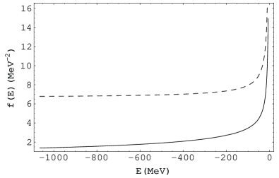
Figure 4: The behavior of the off-shell amplitude $f(E)=10^{9}\langle{\bf p}|T(z)|{\bf p}\rangle$ ($|{\bf p}|=500$ MeV) in the ${}^{3}S_{1}$ channel for $np$ scattering. The solid curve corresponds to the model with a generalized interaction operator (28), compared to the model with Yamaguchi potential with parameters given in Ref. Yam (dashed line).

VI Summary and discussion

In leading order of the EFT approach we have shown that the effective $NN$ interaction is nonlocal in time, and low energy nucleon dynamics is governed by the dynamical Eq. (5) with the nonlocal-in-time interaction operator (43). Thus, in the case of quantum mechanics of nucleons at low energies, we deal with the non-Hamiltonian dynamics that has been investigated in Ref. R.Kh.:1999 . This dynamics is described in a natural way by the GQD that, as has been shown, provides a consistent parametrization of the $NN$ interaction. The leading order contact component of this interaction is parametrized by the nonlocal-in-time operator (43). This operator is well defined, and the generalized dynamical equation with this operator does not requires regularization and renormalization. The parametrization of the $NN$ interaction that takes into account the long-range component is represented by Eq. (51).

The fact that in leading order of the EFT approach low energy nucleon dynamics is described by the model considered in Sec. III allows us to explain the advantages of the GQD in describing nucleon dynamics in terms of this model. As we have shown, the generalized dynamical equation permits any form factor $\varphi({\bf p})$ in Eq. (20) having UV behavior (19) with $\alpha>-\frac{1}{2}$. In the case $\alpha>\frac{1}{2}$, the only possible form of the interaction operator is Eq. (26). In this case we deal with the ordinary separable-potential model. In the case $-\frac{1}{2}<\alpha<\frac{1}{2}$, the interaction operator must be of the form (31), and hence the interaction generating the dynamics of the system is necessarily nonlocal in time. In this case the $T$ matrix is given by Eq. (32). On the other hand, one can obtain the same $T$ matrix in another way, starting with the singular potential

$$V({\bf p}^{\prime},{\bf p})=\lambda\varphi^{*}({\bf p}^{\prime})\varphi({\bf p}),\quad\varphi({\bf p})\sim|{\bf p}|^{-\alpha},\quad\alpha\leq\frac{1}{2}$$ (56)

that does not make sense without renormalization, since it leads to UV divergencies. By solving the $LS$ equation regulated in some way and performing renormalization, one can get expression (32) for the $T$ matrix. However, in this way one cannot determine a potential describing the fundamental interaction in the system. The singular potential (56) is only of formal importance for the problem under consideration. All the information contained in this potential is that the $T$ matrix is of the form $\langle{\bf p}_{2}|T(z)|{\bf p}_{1}\rangle=\varphi^{*}({\bf p}_{2})\varphi({\bf p}_{1})t(z)$ with the same form factor. If the group of the evolution operators given by Eq. (45) had an infinitesimal generator, one could identify it with the Hamiltonian. However, as we have shown in Sec. V, this group has no infinitesimal generator, and hence there are no potentials that could govern the dynamics of the system after renormalization. Moreover, the $T$ matrix (32) does not satisfy the $LS$ equation and has such properties that are at variance with the Hamiltonian formalism. Thus in this case we have only a calculation rule that allows one to compute results for physical quantities. On the other hand, the above problems are the cost of trying to describe the dynamics of the system after renormalization in terms of the Hamiltonian formalism, despite the fact that this dynamics is non-Hamiltonian. From the more general point of view provided by the GQD we see that in this case the $T$ matrix satisfies the generalized dynamical Eq. (II) with the nonlocal-in-time interaction operator (31), and this operator describes the fundamental interaction generating the dynamics of the system. Thus after renormalization in the theory with the potential (56) we have the dynamics that, according to the GQD, must take a place in the case $-\frac{1}{2}<\alpha<\frac{1}{2}$, and an example of such a theory is low energy nucleon dynamics in leading order where the singular potential is $V({\bf p}_{2},{\bf p}_{1})=\widetilde{C}$. Within the GQD this theory is internally consistent and is as well founded as theories with ordinary potentials such as quantum mechanics describing atomic phenomena. For example, the $T$ matrix is well defined, and its properties satisfy the general requirements of the theory. This is not only important from the point of view of the internal consistency of the theory. Only a well-founded theory provides the possibility to obtain, in a theoretical way, new knowledge, and to prove the correctness of calculations performed within its framework. The fact that in the approach based on the GQD we have the well-defined dynamical equation is a great advantage of this approach for practical calculations. This equation does not require regularization and renormalization and is as convenient for numerical calculations as the $LS$ equation.

It is important that the use of the GQD for investigating the dynamical situation in the EFT of nuclear forces gives rise to a natural parametrization of the $NN$ interaction, and uniquely determines the form of the generalized interaction operator describing the interaction of nucleons. In contrast with initial Lagrangians of EFT’s or formal singular potentials that are produced by these Lagrangians, knowing the generalized operator of the $NN$ interaction is sufficient to compute results for physical quantities. We have obtained that in leading order the contact term of the $NN$ interaction is parametrized by the interaction operator (43). In the same order (in Weinberg’s power counting) the $NN$ interaction is parametrized by the operator (54). In this way one can construct the interaction operators in any order of the EFT approach. This operator can then be used, for example, for determining the interaction operators parametrizing interactions of nuclei.

Appendix A

Let us consider the solution of Eq. (II) in the case where the interaction operator is of the form (51). From Eqs. (14) and (15) it follows that this solution can be represented in the form

$$\langle{\bf{p}}_{2}|T(z)|{\bf{p}}_{1}\rangle=\mathop{\rm{lim}}\limits_{u\mathop{\to}-\infty}\langle{\bf{p}}_{2}|T_{u}(z)|{\bf{p}}_{1}\rangle,$$ (57)

where the operator $T_{u}(z)$ is the solution of the equation

$$T_{u}(z)=B(u)+(u-z)B(u)G_{0}(u)G_{0}(z)T_{u}(z).$$ (58)

Here the operator $B(z)$ is given by

$$\langle{\bf p}_{2}|B(z)|{\bf p}_{1}\rangle=f_{1}(z)+V({\bf p}_{2},{\bf p}_{1}),$$ (59)

with

$$f_{1}(z)=-\frac{4\pi}{m^{\frac{3}{2}}\sqrt{-z}}-\frac{16\pi^{2}}{m^{3}C_{0}^{(R)}z}.$$

The solution of Eq. (A2) can be represented in the form

$$\langle{\bf{p}}_{2}|T_{u}(z)|{\bf{p}}_{1}\rangle=t_{0}^{(u)}(z)+t_{1}^{(u)}(z;{\bf{p}}_{1})$$

$$+\widetilde{t}_{1}^{(u)}(z;{\bf{p}}_{2})+t_{2}^{(u)}(z;{\bf{p}}_{1},{\bf{p}}_{2}).$$ (60)

Substituting this representation in Eq. (58) yields the following equations for $t_{0}^{(u)}(z)$, $t_{1}^{(u)}(z;{\bf{p}})$, $\widetilde{t}_{1}^{(u)}(z;{\bf{p}}_{2})$ and $t_{2}^{(u)}(z;{\bf{p}}_{1},{\bf{p}}_{2})$:

$$t_{0}^{(u)}(z)=f_{1}(u)+(u-z)f_{1}(u)$$

$$\times\int\frac{d^{3}k}{(2\pi)^{3}}\frac{\left(t_{0}^{(u)}(z)+t_{1}^{(u)}(z;{\bf k})\right)}{(z-E_{k})(u-E_{k})},$$ (61)

$$t_{1}^{(u)}(z;{\bf p})=(u-z)\int\frac{d^{3}k}{(2\pi)^{3}}\frac{\left(t_{0}^{(u)}(z)+t_{1}^{(u)}(z;{\bf k})\right)}{(z-E_{k})(u-E_{k})}$$

$$\times V({\bf k},{\bf p}),$$ (62)

$$\widetilde{t}_{1}^{(u)}(z;{\bf p})=(u-z)f_{1}(u)$$

$$\times\int\frac{d^{3}k}{(2\pi)^{3}}\frac{\left(\widetilde{t}_{1}^{(u)}(z;{\bf p})+t_{2}^{(u)}(z;{\bf k},{\bf p})\right)}{(z-E_{k})(u-E_{k})},$$ (63)

$$t_{2}^{(u)}(z;{\bf p}_{2},{\bf p}_{1})=V({\bf p}_{2},{\bf p}_{1})+(u-z)\int\frac{d^{3}k}{(2\pi)^{3}}$$

$$\frac{\left(\widetilde{t}_{1}^{(u)}(z;{\bf p}_{2})+t_{2}^{(u)}(z;{\bf p}_{2},{\bf k})\right)}{(z-E_{k})(u-E_{k})}V({\bf k},{\bf p}_{1}).$$ (64)

It is not difficult to verify that

$$t_{1}^{(u)}(z;{\bf p})=\widetilde{t}_{1}^{(u)}(z;{\bf p}).$$

By solving the above set of equations, one can obtain the functions $t_{0}^{(u)}(z)$, $t_{1}^{(u)}(z,{\bf{p}})$ and $t_{2}^{(u)}(z,{\bf{p}}_{2},{\bf{p}}_{1})$ that in turn can be used for constructing the $T$ matrix. In fact, from Eqs. (A1) and (A2) it follows that the $T$ matrix can be represented in the form (49) where the functions $t_{0}(z)$, $t_{1}(z,{\bf{p}})$ and $t_{2}(z,{\bf{p}}_{2},{\bf{p}}_{1})$ are given by

$$t_{0}(z)=\mathop{\rm{lim}}_{u\to-\infty}t_{0}^{(u)}(z),\quad t_{1}(z,{\bf{p}})=\mathop{\rm{lim}}_{u\to-\infty}t_{1}^{(u)}(z,{\bf{p}}),$$

$$t_{2}(z,{\bf{p}}_{2},{\bf{p}}_{1})=\mathop{\rm{lim}}_{u\to-\infty}t_{2}^{(u)}(z,{\bf{p}}_{2},{\bf{p}}_{1}).$$

Taking into account that

$$\int\frac{d^{3}k}{(2\pi)^{3}}\frac{u-z}{(z-E_{k})(u-E_{k})}=\frac{m\sqrt{m}}{4\pi}\left(\sqrt{-z}-\sqrt{-u}\right),$$

equation (61) can be rewritten in the form

$$t_{0}^{(u)}(z)=-\frac{4\pi}{m^{\frac{3}{2}}\sqrt{-u}}+t_{0}^{(u)}(z)$$

$$\times\left(-\frac{4\pi}{m^{\frac{3}{2}}\sqrt{-u}}-\frac{16\pi^{2}}{m^{3}C_{0}^{(R)}u}\right)\frac{m\sqrt{m}}{4\pi}\left(\sqrt{-z}-\sqrt{-u}\right)$$

$$-\frac{4\pi}{m^{\frac{3}{2}}\sqrt{-u}}\int d^{3}k\frac{t_{1}(z,{\bf{k}})}{z-E_{k}}+o(|u|^{-1/2}).$$

Letting $u\to-\infty$ in this equation and assuming that $V({\bf p}_{2},{\bf p}_{1})$ goes to zero sufficiently fast when momenta tend to infinity, one can easily get Eq. (53). In the same way, from Eqs. (62) and (64) one can derive Eqs. (50) and (52).

References

- (1) S. Weinberg, Physica A 96 327 (1979).
- (2) E. Witten, Nucl. Phys. B 122 109 (1977).
- (3) S. Weinberg, Phys. Lett. B 251 288 (1990); Nucl. Phys. B 363 3 (1991).
- (4) C. Ordòñez, and U. van Kolck, Phys. Lett. B 291 459 (1992).
- (5) U. van Kolck, Phys. Rev. C 49 2932 (1994).
- (6) C. Ordòñez, L. Ray, U. van Kolck, Phys. Rev. Lett. 72 1982 (1994); Phys. Rev. C 53 2086 (1996).
- (7) D.B. Kaplan, M.J. Savage, and M.B. Wise, Phys. Lett. B 424 390 (1998); Nucl. Phys. B 534 329 (1998).
- (8) Nuclear Physics with Effective Field Theory II, edited by P.F. Bedaque, M.J. Savage, R. Seki, U. van Kolck (World Scientific, Singapore, 1999); Nuclear Physics with Effective Field Theory, edited by R. Seki, U. van Kolck, M.J. Savage (World Scientific, Singapore, 1998).
- (9) U. van Kolck, Prog. Part. Nucl. Phys. 43, 409 (1999).
- (10) G.P. Lepage, What is Renormalization? (World Scientific, Singapore, 1990); nucl-th/9706029 (unpublished).
- (11) J. Gegelia, Phys. Lett. B 463 133 (1999).
- (12) R.Kh. Gainutdinov, J. Phys. A 32, 5657 (1999).
- (13) R.P. Feynman, Rev. Mod. Phys. 20, 367 (1948); R.P. Feynman and A.R. Hibbs, Quantum Mechanics and Path Integrals (McGraw-Hill, New York, 1965).
- (14) R.Kh. Gainutdinov and A.A. Mutygullina, Yad. Fiz. 62, 2061 (1999).
- (15) U. van Kolck, Nucl. Phys. A 645, 273 (1999)
- (16) R. Kh. Gainutdinov, hep-th/0107139 (unpublished).
- (17) R.Kh. Gainutdinov and A.A. Mutygullina, Yad. Fiz. 65, 1456 (2002).
- (18) Y.Yamaguchi, Phys. Rev. 95, 1635 (1954).
- (19) D.R. Phillips, I.R. Afnan, and A.G. Henry-Edwards, Phys. Rev. C. 61, 044002-1 (2000).
- (20) V.G.J. Stoks, R.A.M. Klomp, M.C.M. Rentmeester, and J.J. de Swart, Phys. Rev. C 48, 792 (1993).