An isobar model for $\bm{\eta}$ photo- and electroproduction on the nucleon

Abstract

Eta photo- and electroproduction on the nucleon is studied using an isobar model. The model contains Born terms, and contributions from vector meson exchanges and nucleon resonances. Our results are compared with recent eta photoproduction data for differential and total cross sections, beam asymmetry, and target asymmetry, as well as electroproduction data. Besides the dominant $S_{11}(1535)$ resonance, we show that the second $S_{11}$ resonance, $S_{11}(1650)$, is also necessary to be included in order to extract $S_{11}(1535)$ resonance parameters properly. In addition, the beam asymmetry data allow us to extract very small ($<0.1\%$) $N^{*}\rightarrow\eta N$ decay branching ratios of the $D_{13}(1520)$ and $F_{15}(1680)$ resonances because of the overwhelming $s$-wave dominance. This model (ETA-MAID) is implemented as a part of the MAID program .

1 Introduction

Eta photo- and electroproduction on the nucleon, $\gamma^{*}N\rightarrow\eta N$, provide an alternative tool to study $N^{*}$ besides $\pi N$ scattering and pion photoproduction. There are fewer resonances involved since the $\eta N$ state couples to nucleon resonances with isospin $I=1/2$ only. Therefore, this process is cleaner and more selective to distinguish certain resonances than other processes, e.g., pion photoproduction. This provides opportunities to access less studied resonances and possibly the “missing resonances”.

During the last decade eta photo- and electroproduction has been studied in very different frameworks. Common in most approaches is the dominance of the $S_{11}(1535)$ resonance, which seems to be the natural mechanism to describe the almost constant angular distributions of the differential cross sections from threshold at $W=1487\;\mathrm{MeV}$ up to energies around $W=1700\;\mathrm{MeV}$. Early coupled channel approaches predicted eta photoproduction on the basis of elastic and inelastic pion nucleon scattering and pion photoproduction amplitudes [1], more recent developments included the eta photoproduction data in their fits [2, 3, 4]. Field theoretical Lagrangian models [5, 6, 7] and applications of chiral perturbation theory [8, 9] derive covariant eta production amplitudes from Born terms, vector meson exchange, and resonance excitations. In these approaches the spin 3/2 resonances such as $D_{13}(1520)$ are treated in a Rarita-Schwinger formalism but higher spin resonances have not yet been introduced. Relativistic quark models have been successful in describing the general behavior of the cross sections [10, 11], and in a very recent approach a very good fit of the existing data has been obtained by introducing a third $S_{11}$ resonance around 1700 MeV [12] in addition to the well-known resonances $S_{11}(1535)$ and $S_{11}(1650)$. The role of polarization observables has been studied in an isobar model [13] based on early experiments from Bonn [14] and Mainz [15].

Apart from the $S_{11}(1535)$ dominated approaches, alternative ways have been discussed within the Lee Model as well as in chiral meson-baryon Lagrangian theory. In these approaches the $s$-wave production is either described by a nonresonant background [16] or by a molecule like $K\Sigma$ intermediate state. As was pointed out by Höhler [17, 18], the existence of the $S_{11}(1535)$ cannot be unambiguously proven by the standard technique of pion nucleon speed-plots. A pole position of $1505-85i$ as given by PDG [19] is too close to threshold with a width larger than the distance from threshold in order to show a peak in the speed-plot. The only signature that appears is the sharp spike due to the $\eta$ cusp. On the other hand the resonance is strongly supported by the quark model and even the large $\eta N$ branching ratio of almost 50% can be understood by color hyperfine mixing [20]. The same resonance also makes a significant contribution in pion photo- and electroproduction. There, however, it usually causes the problem of a photon resonance coupling $A_{1/2}$ of only $0.5-0.6$ times the value obtained in eta photoproduction analyses [5, 21]. In order to shed more light on the underlying nature of the very pronounced $s$-wave amplitude, a precise study of the $Q^{2}$ dependence of both transverse and longitudinal couplings is needed for both pion and eta electroproduction. In addition the same mechanism also has to describe the eta production off neutrons that has been investigated in coherent and incoherent eta photoproduction experiments on the deuteron. Only by introducing a strong background in the $s$-wave amplitude both reactions could be described simultaneously [22].

The situation of higher resonances is somewhat different. Their existence is well established but the decay in the $\eta N$ channel is mostly very vague. Branching ratios listed in PDG92 were later removed for being too uncertain. Only very recently, due to precise photon asymmetry data from GRAAL, a branching ratio of $(0.08\pm 0.01)\%$ could be determined for the $D_{13}(1520)$ resonance [23]. This result has also been confirmed by other analyses of the same data set. In these analyses another discrepancy in comparison to pion photoproduction was observed yielding a much smaller $A_{3/2}/A_{1/2}$ ratio for the $D_{13}(1520)$ resonance [6, 23, 24].

Unlike pion production for which Born terms give large background contributions to all partial waves due to the large pion nucleon coupling constant, in $\eta$ production the coupling of the eta meson to the nucleon is very small. Already in the SU(3) limit the coupling $g_{\eta NN}^{2}/4\pi=0.8-1.9$ is much smaller than for pions ($g_{\pi NN}^{2}/4\pi=14.3$), but in an analysis of the angular distributions of eta photoproduction an even smaller value of $g_{\eta NN}^{2}/4\pi=0.4\pm 0.2$ was determined [25]. Such a small value was later also explained within a chiral Lagrangian approach [26, 27], and in a very recent fit within a chiral constituent quark model a value of only $0.04$ has been obtained [12]. Therefore, the only sizeable background contribution remains in the $t$-channel vector meson amplitudes, mainly due to $\rho^{0}$ exchange.

The aim of this paper is to extend an earlier version of an isobar model by Knöchlein et al. [13] and to continue the work on the unitary isobar model MAID [28]. In the same way as in MAID for pions we will describe the eta photo- and electroproduction in terms of nucleon Born terms, vector meson exchange contributions and resonance excitations parameterized with Breit-Wigner shapes directly connected to the conventional resonance parameters listed in the particle data tables: masses, widths, branching ratios and photon couplings. By use of the world data on photo- and electroproduction, all free or uncertain parameters of the model will be fixed by least squares fitting. These data are the total and differential photoproduction cross sections of MAMI [15] and GRAAL [29], the photon asymmetry of GRAAL [30] and the electroproduction cross sections of JLab [31, 32].

In Section 2, we give the general formalism of photo- and electroproduction, and describe the model ingredients and resonance parameterization in Section 3. Our fitting results and predictions for future experiments are given in Section 4 followed by a summary and conclusions.

2 Formalism

Consider $\eta$ electromagnetic production on the nucleon. This reaction includes (1) photoproduction

$$\gamma\,(k)+N\,(p_{i})\longrightarrow\eta\,(q)+N\,(p_{f})\,,$$ (1)

and (2) electroproduction

$$e\,(k_{i})+N\,(p_{i})\longrightarrow e^{\prime}\,(k_{f})+\eta\,(q)+N\,(p_{f})\,,$$ (2)

where the four-momentum for each particle is indicated in the parentheses. The four-momentum of the virtual photon exchanged in electroproduction is given by $k=k_{i}-k_{f}$, with $k^{2}=0$ for photoproduction. The four-momentum square of the virtual photon is negative; therefore, in this context we use a positive quantity $Q^{2}\equiv-k^{2}=\bm{k}^{2}-\omega^{2}$ to describe form factors and structure functions.

In the $\gamma N/\eta N$ center-of-mass (c.m.) frame, the momenta of the initial $\gamma N$ and final $\eta N$ states can be expressed in terms of the total c.m. energy $W=\sqrt{s}$ and $k^{2}$,

$$|\bm{k}|=|\bm{p_{i}\,}| = \frac{1}{2W}\sqrt{\bigl{(}(W+M_{i}\,)^{2}+Q^{2}\bigr{)}\bigl{(}(W-M_{i}\,)^{2}+Q^{2}\bigr{)}}\,,$$

$$|\bm{q}|=|\bm{p_{f}}| = \frac{1}{2W}\sqrt{\bigl{(}(W+M_{f})^{2}-m^{2}\bigr{)}\bigl{(}(W-M_{f})^{2}-m^{2}\bigr{)}}\,.$$ (3)

In photoproduction, the relation between the photon energy $E_{\gamma}^{lab}$ in the lab frame and the total c.m. energy $W$ is

$$E_{\gamma}^{lab}=\frac{W^{2}-M_{i}^{2}}{2M_{i}}\,.$$ (4)

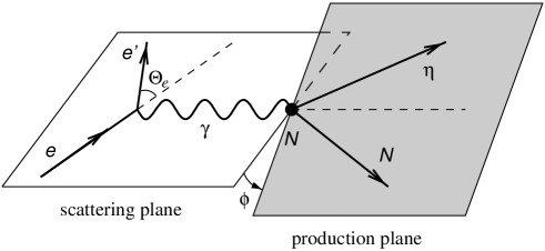
Figure 1: Kinematics in the lab frame for $\eta$ electroproduction $eN\rightarrow e^{\prime}\eta N$

Following the convention of Bjorken and Drell [33], the differential cross section for the electroproduction process can be written as

$$\d\sigma = \frac{m_{e}M_{i}}{\sqrt{(k_{i}\cdot p_{i})^{2}-k_{i}^{2}\,p_{i}^{2}}}\frac{d^{3}k_{f}}{(2\pi)^{3}}\frac{m_{e}}{\varepsilon_{f}}\frac{d^{3}q}{(2\pi)^{3}}\frac{1}{2\omega_{\eta}}\frac{d^{3}p_{f}}{(2\pi)^{3}}\frac{M_{f}}{E_{f}}$$ (5)

$$\times(2\pi)^{4}\,\delta^{(4)}(k+p_{i}-q-p_{f})\,\bigl{|}\langle\,p_{f}\,q\,|\,J^{\mu}\,|\,p_{i}\,\rangle\frac{1}{\;k^{2}\,}\langle\,k_{f}\,|\,j_{\mu}\,|\,k_{i}\,\rangle\bigr{|}^{2}\;,$$

where $j^{\mu}$ and $J^{\mu}$ denote the electromagnetic currents of the electron and the hadronic system, respectively.

The transverse polarization parameter of the virtual photon

$$\varepsilon=\left(1+2\frac{\,\bm{k}^{2}}{\,Q^{2}}\tan^{2}\frac{\Theta_{e}}{2}\right)^{-1}\,,$$ (6)

is invariant under collinear transformations, and $\bm{k}$ and $\Theta_{e}$ may be expressed in the lab or c.m. frame. By choosing the energies of the initial and final electrons and the scattering angle $\Theta_{e}$ (see Fig. 1), we can fix the momentum transfer $Q^{2}$ and the polarization parameter $\varepsilon$ of the virtual photon.

The five-fold differential cross section for electroproduction can be expressed as [34, 35, 36]

$$\frac{\d\sigma}{\d\Omega_{f}\,\d\varepsilon_{f}\,\d\Omega}=\Gamma\,\frac{\d\sigma_{v}}{\d\Omega}\,,$$ (7)

with the flux of the virtual photon field given by

$$\Gamma=\frac{\alpha}{2\pi^{2}}\,\frac{\varepsilon_{f}}{\varepsilon_{i}}\,K\,\frac{1}{1-\varepsilon}\,,$$ (8)

where $\varepsilon_{i}$ and $\varepsilon_{f}$ are the initial and final electron energies. In this expression $K\equiv(W^{2}-M_{i}^{2})/2M_{i}$ denotes the “photon equivalent energy”, the laboratory energy necessary for a real photon to excite a hadronic system with c.m. energy $W$. It is useful to express the angular distribution of the eta mesons in the c.m. frame of the final hadronic states, particularly for the use of multipole decompositions. Therefore, the virtual photon cross section $\d\sigma_{v}/\d\Omega$ should be evaluated in the c.m. frame, while the five-fold differential cross section in the Eq. (7) is interpreted with the flux factor in the lab frame. For the rest of the paper we only use c.m. variables.

For an unpolarized target and without recoil polarization, the virtual photon differential cross section is

$$\frac{\d\sigma_{v}}{\d\Omega} = \frac{\d\sigma_{T}}{\d\Omega}+\varepsilon\,\frac{\d\sigma_{L}}{\d\Omega}+\sqrt{2\varepsilon(1+\varepsilon)}\;\frac{\d\sigma_{LT}}{\d\Omega}\,\cos\phi$$ (9)

$$+\varepsilon\,\frac{\d\sigma_{TT}}{\d\Omega}\,\cos 2\phi+h\,\sqrt{2\varepsilon(1-\varepsilon)}\;\frac{\d\sigma_{LT^{\prime}}}{\d\Omega}\,\sin\phi\,.$$

Here $\phi$ is the azimuthal angle between the electron scattering plane and the $\eta$ production plane (see Fig. 1), and $h=\bm{\sigma}\cdot\hat{\bm{k}}_{i}=\pm 1$ is the helicity of the incident electron with longitudinal polarization. The first two terms ($\d\sigma_{T}$ and $\d\sigma_{L}$) in the RHS of Eq. (9) are referred as the transverse and longitudinal cross sections, and do not depend on the azimuthal angle $\phi$. The $\d\sigma_{LT}$ and $\d\sigma_{LT^{\prime}}$ describe longitudinal-transverse interferences, and the $\d\sigma_{TT}$ is a transverse-transverse interference term. We do not use the longitudinal polarization $\varepsilon_{L}$; therefore, the cross sections with longitudinal components ($\d\sigma_{L}$, $\d\sigma_{LT}$ and $\d\sigma_{LT^{\prime}}$) differ from those in Refs. [13, 36].

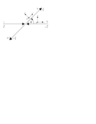
Figure 2: Frames for polarization vectors in $\eta$ photoproduction in the c.m. system

Three types of polarization measurements can be performed in pseudoscalar meson production: photon beam polarization, polarization of the target nucleon, and polarization of the recoil nucleon. Target polarization is described in the frame $\{x,y,z\}$ of Fig. 2, with the $z$-axis pointing into the direction of the photon momentum $\hat{\bm{k}}$, the $y$-axis perpendicular to the reaction plane, $\hat{\bm{y}}=\hat{\bm{k}}\times\hat{\bm{q}}/\sin\theta$, and the $x$-axis given by $\hat{\bm{x}}=\hat{\bm{y}}\times\hat{\bm{z}}$. For recoil polarization we will use the frame $\{x^{\prime},y^{\prime},z^{\prime}\}$, with the $z^{\prime}$-axis defined by the outgoing $\eta$ momentum vector $\hat{\bm{q}}$, the $y^{\prime}$-axis as for target polarization and the $x^{\prime}$-axis given by $\hat{\bm{x}}^{\prime}=\hat{\bm{y}}^{\prime}\times\hat{\bm{z}}^{\prime}$. The most general expression for a coincidence experiment considering all three types of polarization is

$$\frac{\d\sigma_{v}}{\d\Omega} = \frac{|\,\bm{q}\,|}{|\,\bm{k}\,|}P_{\alpha}P_{\beta}\Bigl{\{}R_{T}^{\beta\alpha}+\varepsilon\,\tfrac{Q^{2}}{\omega^{2}}R_{L}^{\beta\alpha}$$ (10)

$$+\,\sqrt{2\,\varepsilon(1+\varepsilon)\tfrac{Q^{2}}{\omega^{2}}}\,\bigl{(}{\,}^{c}\!R_{LT}^{\beta\alpha}\cos\phi+{\,}^{s}\!R_{LT}^{\beta\alpha}\sin\phi\bigr{)}$$

$$+\,\varepsilon\,\bigl{(}{\,}^{c}\!R_{TT}^{\beta\alpha}\cos 2\phi+{\,}^{s}\!R_{TT}^{\beta\alpha}\sin 2\phi\bigr{)}$$

$$+\,h\,\sqrt{2\,\varepsilon(1-\varepsilon)\tfrac{Q^{2}}{\omega^{2}}}\,\bigl{(}{\,}^{c}\!R_{LT^{\prime}}^{\beta\alpha}\cos\phi+{\,}^{s}\!R_{LT^{\prime}}^{\beta\alpha}\sin\phi\bigr{)}$$

$$+\,h\,\sqrt{1-\varepsilon^{2}}\,R_{TT^{\prime}}^{\beta\alpha}\Bigr{\}}\,,$$

where $P_{\alpha}=(1,\bm{P})$ and $P_{\beta}=(1,\bm{P}^{\prime})$. Here $\bm{P}=(P_{x},P_{y},P_{z})$ and $\bm{P}^{\prime}=(P_{x^{\prime}},P_{y^{\prime}},P_{z^{\prime}})$ denotes the target and recoil polarization vector. The zero components $P_{0}=1$ correspond to contributions in the cross section which are present in the polarized as well as the unpolarized case. In an experiment without target and recoil polarization $\alpha=\beta=0$, therefore the only remaining contributions are $R_{i}^{00}$. The functions $R_{i}^{\beta\alpha}$ describe the response of the hadronic system in the process. Summation over Greek indices is implied. An additional superscript $s$ or $c$ on the left indicates a sine or cosine dependence of the respective contribution on the azimuthal angle. Some response functions vanish identically. See Ref. [13] for a systematic overview.

In photoproduction the longitudinal components vanish due to the external factors $\sqrt{Q^{2}/\omega^{2}}$ ($\omega$ is the c.m. energy of the virtual photon), and in the following the relevant response functions will be divided by the (unpolarized) transverse response function $R_{T}^{00}$ in order to obtain the polarization observables. The common descriptors of these observables can be found in Table 1.

Table 1: Polarization observables in pseudoscalar meson photoproduction. The entries in parentheses signify that the same polarization observables also appear elsewhere in the table.

Photon		Target			Recoil			Target + Recoil
	$-$	$-$	$-$	$-$	$x^{\prime}$	$y^{\prime}$	$z^{\prime}$	$x^{\prime}$	$x^{\prime}$	$z^{\prime}$	$z^{\prime}$
	$-$	$x$	$y$	$z$	$-$	$-$	$-$	$x$	$z$	$x$	$z$
unpolarized	$\sigma_{0}$	$0$	$T$	$0$	$0$	$P$	$0$	$T_{x^{\prime}}$	​$-L_{x^{\prime}}$​	$T_{z^{\prime}}$	$L_{z^{\prime}}$
linear pol.	$\ -\Sigma\$	$\ H\$	​$(-P)$​	$-G$	$\ O_{x^{\prime}}$	​​$(-T)$​​	$\ O_{z^{\prime}}$	​$(-L_{z^{\prime}})$​	​​$(\,T_{z^{\prime}}\,)$​​	​$(-L_{x^{\prime}})$​	​​$(-T_{x^{\prime}})$​​
circular pol.	$\quad 0\quad$	$F$	$0$	$-E$	$-C_{x^{\prime}}$	$0$	$-C_{z^{\prime}}$	$0$	$0$	$0$	$0$

In contrast to electroproduction, there are no new independent polarization observables accessible by triple (beam + target + recoil) polarization measurements in photoproduction. As a consequence we classify the differential cross sections by the three classes of double polarization experiments:

• polarized photons and polarized target

$$\frac{\d\sigma}{\d\Omega} = \sigma_{0}\bigl{[}\,1-P_{T\,}\Sigma\cos 2\varphi+P_{x}(-P_{T}H\sin 2\varphi+P_{\odot}F)$$ (11)

$$-P_{y}(-T+P_{T}P\cos 2\varphi)-P_{z}(-P_{T}G\sin 2\varphi+P_{\odot}E)\bigr{]}\,,$$

• polarized photons and recoil polarization

$$\frac{\d\sigma}{\d\Omega} = \sigma_{0}\bigl{[}\,1-P_{T\,}\Sigma\cos 2\varphi+P_{x^{\prime}}(-P_{T}O_{x^{\prime}}\sin 2\varphi-P_{\odot}C_{x^{\prime}})$$ (12)

$$-P_{y^{\prime}}(-P+P_{T}T\cos 2\varphi)-P_{z^{\prime}}(P_{T}O_{z^{\prime}}\sin 2\varphi+P_{\odot}C_{z^{\prime}})\bigr{]}\,,$$

• polarized target and recoil polarization

$$\frac{\d\sigma}{\d\Omega} = \sigma_{0}\bigl{[}\,1+P_{y^{\prime}}P+P_{x}(P_{x^{\prime}}T_{x^{\prime}}+P_{z^{\prime}}T_{z^{\prime}})$$ (13)

$$+P_{y}(T+P_{y^{\prime}}\Sigma)-P_{z}\left(P_{x^{\prime}}L_{x^{\prime}}-P_{z^{\prime}}L_{z^{\prime}}\right)\bigr{]}\,,$$

where $\sigma_{0}$ denotes the unpolarized differential cross section, $P_{T}$ the transverse degree of photon polarization, $P_{\odot}$ the right-handed circular photon polarization, and $\varphi$ the angle between photon polarization vector and reaction plane.

In conclusion, there are 16 different polarization observables for real photon experiments. In electroproduction there are four additional observables for the exchange of longitudinal photons and sixteen observables due to longitudinal-transverse interference. However, there are only six independent complex amplitudes for the electroproduction process. This corresponds to six absolute values and five relative phases between the CGLN amplitudes; i.e. there are only eleven independent quantities which completely and uniquely determine the transition current $J^{\mu}$.

The aim of a so-called “complete experiment” is to fully determine the current $J^{\mu}$ for the process under investigation in a given kinematics. For the photoproduction case a minimum of eight carefully chosen observables can determine amplitudes without any ambiguities [37]. Although it would be interesting to pursue such a project for $\eta$ production, we will concentrate on the more physical aspects of this process. In particular our theoretical investigations will supply information on an adequate selection of response functions and observables. In the case of $\eta$ production it will be of special interest to study observables which give clear information of the eta meson coupling to higher resonances.

We can also introduce amplitudes defined by the helicity eigenstates of the initial and final nucleons and the photon in photoproduction [38]. The connections between the helicity amplitudes $H_{i}$ and the CGLN amplitudes $\mathcal{F}_{i}$ are

$$H_{1}(\theta) = -\tfrac{1}{\sqrt{2}}\,\sin\theta\,\cos\tfrac{\theta}{2}\,\bigl{(}\mathcal{F}_{3}+\mathcal{F}_{4}\bigr{)}\,e^{i\phi}\,,$$

$$H_{2}(\theta) = \sqrt{2}\,\cos\tfrac{\theta}{2}\,\bigl{[}(\mathcal{F}_{2}-\mathcal{F}_{1})+\sin^{2}\tfrac{\theta}{2}\,(\mathcal{F}_{3}-\mathcal{F}_{4})\bigr{]}\,,$$

$$H_{3}(\theta) = \tfrac{1}{\sqrt{2}}\,\sin\theta\,\sin\tfrac{\theta}{2}\,\bigl{(}\mathcal{F}_{3}-\mathcal{F}_{4}\bigr{)}\,e^{2i\phi}\,,$$

$$H_{4}(\theta) = \sqrt{2}\,\sin\tfrac{\theta}{2}\,\bigl{[}(\mathcal{F}_{2}+\mathcal{F}_{1})+\cos^{2}\tfrac{\theta}{2}\,(\mathcal{F}_{3}+\mathcal{F}_{4})\bigr{]}\,e^{i\phi}\,,$$

$$H_{5}(\theta) = \cos\tfrac{\theta}{2}\,\bigl{(}\mathcal{F}_{6}+\mathcal{F}_{5}\bigr{)}\,,$$

$$H_{6}(\theta) = \sin\tfrac{\theta}{2}\,\bigl{(}\mathcal{F}_{6}-\mathcal{F}_{5}\bigr{)}\,e^{i\phi}\,.$$ (14)

3 Isobar model

The isobar model used in this work is closely related to the unitary isobar model (MAID) developed by Drechsel et al. [28]. The major difference is that in MAID, which deals with pion photo- and electroproduction, the phases of the multipole amplitudes are adjusted to the corresponding pion-nucleon elastic scattering phases. However, in $\eta$ production the unitarization procedure is not feasible, because the necessary information on eta-nucleon scattering is not available.

3.1 Background

The nonresonant background contains the usual Born terms and vector meson exchange contributions. It is obtained by evaluating the Feynman diagrams derived from an effective Lagrangian. For the electromagnetic $\gamma NN$ vertex the structure is well understood,

$$\mathcal{L}_{\gamma NN}=-e\,\bar{\psi}\left[\gamma_{\mu}A^{\mu}F_{1}^{p,n}(Q^{2})+\frac{\sigma_{\mu\nu}}{2m_{N}}(\partial^{\mu}A^{\nu})F_{2}^{p,n}(Q^{2})\right]\psi\,,$$ (15)

with $A^{\mu}$ the electromagnetic vector potential, and $\psi$ the nucleon field operators. In Eq. (15) we have included proton ($F_{1,2}^{p}$) and neutron ($F_{1,2}^{n}$) electromagnetic form factors with explicit $Q^{2}$ dependence. In the case of real photons the form factors are normalized to $F_{1}^{p}(0)=1$, $F_{1}^{n}(0)=0$, $F_{2}^{p}(0)=\kappa_{p}=1.79$ and $F_{2}^{n}(0)=\kappa_{n}=-1.97$. For virtual photons the nucleon form factors are expressed in terms of the Sachs form factors by the standard dipole form, $F_{D}(Q^{2})=(1+Q^{2}/0.71(\mbox{GeV/c})^{2})^{-2}$

The description of the hadronic $\eta NN$ vertex is more sophisticated in the pseudoscalar meson electroproduction. There are two possibilities for constructing the interaction Lagrangian, namely, the pseudoscalar (PS) coupling,

$$\mathcal{L}_{\eta NN}^{PS}=-i\,g_{\eta NN}\,\bar{\psi}\,\gamma_{5}\,\psi\,\phi_{\eta}\,,$$ (16)

and the pseudovector (PV) coupling,

$$\mathcal{L}_{\eta NN}^{PV}=\frac{f_{\eta NN}}{m_{\eta}}\,\bar{\psi}\,\gamma_{5}\,\gamma_{\mu}\,\psi\,\partial^{\mu}\phi_{\eta}\,,$$ (17)

where the two types of coupling are related by $f_{\eta NN}/m_{\eta}=g_{\eta NN}/2m_{N}$. In contrast to the $\pi N$ interaction, where PS coupling is ruled out by chiral symmetry, both couplings are allowed for the $\eta N$ interaction and we have chosen the PS coupling in accordance with Ref. [25].

Using the effective Lagrangians Eqs. (15)-(17), we construct the usual Born terms. The other part of background is vector meson exchange contributions. The effective Lagrangians for the vector meson exchange vertices are

$${\mathcal{L}}_{\gamma\eta V} = \frac{e\lambda_{V}}{m_{\eta}}\,\varepsilon_{\mu\nu\rho\sigma}\,(\partial^{\mu}A^{\nu})\,\phi_{\eta}\,(\partial^{\rho}V^{\sigma})\,F_{V}^{em}(Q^{2})\,,$$ (18)

$${\mathcal{L}}_{VNN} = {\bar{\psi}}\left(g_{v}\gamma_{\mu}+\frac{g_{t}}{2m_{N}}\,\sigma_{\mu\nu}\partial^{\nu}\right)V^{\mu}\psi\,,$$ (19)

The parameters for the $\rho$ and $\omega$ mesons in this model are listed in Table 2. The electromagnetic couplings of the vector mesons $\lambda_{V}$ are determined from the radiative decay widths $\Gamma_{V\rightarrow\eta\gamma}$ via

$$\Gamma_{V\rightarrow\eta\gamma}=\frac{\alpha(m_{V}^{2}-m_{\eta}^{2})^{3}}{24\,m_{V}^{3}\,m_{\eta}^{2}}\,\lambda_{V}^{2}\,,$$ (20)

and the electromagnetic form factor $F_{V}^{em}(Q^{2})$ is assumed to have the usual dipole behavior. The off-shell behavior of the hadronic couplings $g_{v}$ (vector coupling) and $g_{t}$ (tensor coupling) in Eq. (19) is described by a dipole form factor

$$g_{v,\,t}=\tilde{g}_{v,\,t}\,\frac{\left(\Lambda_{V}^{2}-m_{V}^{2}\right)^{2}}{\left(\Lambda_{V}^{2}+\bm{k}_{V}^{2}\right)^{2}}\,.$$ (21)

In general the values for the strong coupling constants $\tilde{g}_{v}$ and $\tilde{g}_{t}$ are not well determined. In various analyses [28, 39, 40] they vary in the ranges of $1.8\leq\tilde{g}^{\rho}_{v}\leq 3.2$, $8\leq\tilde{g}^{\omega}_{v}\leq 20$, $4.3\leq\tilde{g}^{\rho}_{t}/\tilde{g}^{\rho}_{v}\leq 6.6$, and $-1\leq\tilde{g}^{\omega}_{t}/\tilde{g}^{\omega}_{v}\leq 0$. In the present work we take them as free parameters to be varied within these ranges. The fitted values of these parameters are given in Table 2.

Table 2: Parameters for the vector mesons.

$V$	$m_{V}\,[{\mathrm{M}eV}]$	$\tilde{g}_{v}$	$\tilde{g}_{t}/\tilde{g}_{v}$	$\Lambda_{V}\,[{\mathrm{G}eV}]$	$\lambda_{V}$
$\rho$	$768.5$	$2.4$	$6.1$	$1.3$	$0.810$
$\omega$	$782.6$	$16$	$0$	$1.3$	$0.291$

3.2 Resonance contribution

In addition to the dominant $S_{11}(1535)$, we also consider $N^{*}$ contributions from $D_{13}(1520)$, $S_{11}(1650)$, $D_{15}(1675)$, $F_{15}(1680)$, $D_{13}(1700)$, $P_{11}(1710)$, and $P_{13}(1720)$. For the relevant multipoles $\mathcal{M}_{\ell\pm}$ ($=E_{\ell\pm},\,M_{\ell\pm},\,S_{\ell\pm}$) of the resonance contributions, we assume a Breit-Wigner energy dependence of the form

$$\mathcal{M}_{\ell\pm}(W,Q^{2})=\tilde{\mathcal{M}}_{\ell\pm}(Q^{2})\,\frac{W_{R}\Gamma_{\mathrm{tot}}(W)}{W_{R}^{2}-W^{2}-iW_{R}\Gamma_{\mathrm{tot}}(W)}\,f_{\eta N}(W)\,C_{\eta N}\,,$$ (22)

where $f_{\eta N}(W)$ is the usual Breit-Wigner factor describing the $\eta N$ decay of the $N^{*}$ resonance with total width $\Gamma_{\mathrm{tot}}$, partial width $\Gamma_{\eta N}$ and spin $J$,

$$f_{\eta N}(W)=\zeta_{\eta N}\left[\frac{1}{(2J+1)\pi}\,\frac{k_{W}}{|\,\bm{q}\,|}\,\frac{m_{N}}{W_{R}}\,\frac{\Gamma_{\eta N}}{\Gamma_{\mathrm{tot}}^{2}}\right]^{1/2},\quad k_{W}=\frac{W^{2}-m_{N}^{2}}{2W}\,,$$ (23)

where $\zeta_{\eta N}=\pm 1$ describes the relative sign between $N^{*}\rightarrow\eta N$ and $N^{*}\rightarrow\pi N$ couplings. The isospin factor $C_{\eta N}$ is $-1$, and $\tilde{E}_{\ell\pm}$, $\tilde{M}_{\ell\pm}$ and $\tilde{S}_{\ell\pm}$ are related to the photon excitation helicity amplitudes by

$$A^{\ell+}_{1/2} = -\frac{1}{2}\,\bigl{[}(\ell+2)\tilde{E}_{\ell+}+\ell\,\tilde{M}_{\ell+}\bigr{]},$$

$$A^{\ell+}_{3/2} = \frac{1}{2}\,\sqrt{\ell(\ell+2)}\,\bigl{(}\tilde{E}_{\ell+}-\tilde{M}_{\ell+}\bigr{)},$$

$$A^{(\ell+1)-}_{1/2} = -\frac{1}{2}\,\bigl{[}\ell\,\tilde{E}_{(\ell+1)-}-(\ell+2)\tilde{M}_{(\ell+1)-}\bigr{]},$$

$$A^{(\ell+1)-}_{3/2} = -\frac{1}{2}\,\sqrt{\ell(\ell+2)}\,\bigl{(}\tilde{E}_{(\ell+1)-}+\tilde{M}_{(\ell+1)-}\bigr{)},$$

$$S^{\ell+}_{1/2} = -\frac{1}{\sqrt{2}}\,(\ell+1)\,\tilde{S}_{\ell+}\,,$$

$$S^{(\ell+1)-}_{1/2} = -\frac{1}{\sqrt{2}}\,(\ell+1)\,\tilde{S}_{(\ell+1)-}\,.$$ (24)

The scalar multipole amplitudes $S_{\ell\pm}$ appear only in electroproduction, and are related to the longitudinal ones by $\omega S_{\ell\pm}=|\bm{k}|L_{\ell\pm}$.

In accordance with Ref. [38], the energy dependence of the partial width $\Gamma_{\eta N}$ is given by

$$\Gamma_{\eta N}(W)=\beta_{\eta N}\,\Gamma_{R}\left(\frac{|\;\bm{q}\;|}{|\bm{q}_{R}|}\right)^{2\ell+1}\left(\frac{X^{2}+\bm{q}_{R}^{2}}{X^{2}+\bm{q}^{2}}\right)^{\ell}\frac{W_{R}}{W}\,,$$ (25)

where $X$ is a damping parameter, assumed to be $500$ MeV for all resonances. $\Gamma_{R}$ and $q_{R}$ are the total width and the $\eta$ c.m. momentum at the resonance peak ($W=W_{R}$) respectively, and $\beta_{\eta N}$ is the $\eta N$ decay branching ratio.

The total width $\Gamma_{\mathrm{tot}}$ in Eqs. (22) and (23) is the sum of $\Gamma_{\eta N}$, the single-pion decay width $\Gamma_{\pi N}$, and the rest, for which we assume dominance of the two-pion decay channels,

$$\Gamma_{\mathrm{tot}}(W)=\Gamma_{\eta N}(W)+\Gamma_{\pi N}(W)+\Gamma_{\pi\pi N}(W)\,.$$ (26)

The width $\Gamma_{\pi N}$ has a similar energy dependence as $\Gamma_{\eta N}$, and $\Gamma_{\pi\pi N}$ is parameterized in an energy dependent form,

$$\Gamma_{\pi N}(W) = \beta_{\pi N}\,\Gamma_{R}\left(\frac{|\bm{q_{\pi}}|}{|\bm{q}_{R}|}\right)^{2\ell+1}\left(\frac{X^{2}+\bm{q}_{R}^{2}}{X^{2}+\bm{q_{\pi}}^{2}}\right)^{\ell}\frac{W_{R}}{W}\,,$$ (27)

$$\Gamma_{\pi\pi N}(W) = (1-\beta_{\pi N}-\beta_{\eta N})\,\Gamma_{R}\left(\frac{q_{2\pi}}{q_{0}}\right)^{2\ell+4}\left(\frac{X^{2}+q_{0}^{2}}{X^{2}+q_{2\pi}^{2}}\right)^{\ell+2},$$ (28)

where $q_{2\pi}$ is the momentum of the compound (2$\pi$) system with mass $2m_{\pi}$ and $q_{0}=q_{2\pi}$ at $W=W_{R}$. The definition of $\Gamma_{\pi\pi N}$ has been chosen to account for the correct energy behavior of the phase space near the three-body threshold.

Table 3: Parameters of nucleon resonances studied in our isobar model. The masses and widths are given in MeV, $\zeta_{\eta N}$ give the relative sign between $N^{*}\rightarrow\eta N$ and $N^{*}\rightarrow\pi N$ couplings, and $\beta_{\eta N,\,\pi N,\,\pi\pi N}$ are the branching ratios for the respective decay channels. In the first row for each resonance, we list the average values or ranges given by the Particle Data Group (PDG) [19]. The numbers in the second rows are the values used in our model, the underlined ones being taken as free parameters determined from data fitting. If no value is shown in the second rows, then the PDG value is adopted.

$N^{*}$	Mass	Width	$\zeta_{\eta N}$	$\beta_{\eta N}$	$\beta_{\pi N}$	$\beta_{\pi\pi N}$
$D_{13}(1520)$	1520	120	$+1$	$0.08\pm 0.01\%$	$50-60\%$	$40-50\%$
				$0.06\%$	$60\%$	$40\%$
$S_{11}(1535)$	1520-1555	100-250	$+1$	$30-55\%$	$35-55\%$	$1-10\%$
	1541	191		$50\%$	$40\%$	$10\%$
$S_{11}(1650)$	1640-1680	145-190	$-1$	$3-10\%$	$55-90\%$	$10-20\%$
	1638	114		$7.9\%$	$77\%$	$15\%$
$D_{15}(1675)$	1670-1685	150	$-1$	$0.1\pm 0.1\%$	$40-50\%$	$50-60\%$
	1665			$17\%$	$40\%$	$43\%$
$F_{15}(1680)$	1675-1690	130	$+1$	$0.15\pm 0.3\%$	$60-70\%$	$30-40\%$
	1681			$0.06\%$	$60\%$	$40\%$
$D_{13}(1700)$	1700	100	$-1$	$10\pm 6\%$	$5-15\%$	$85-95\%$
				$0.3\%$	$15\%$	$85\%$
$P_{11}(1710)$	1680-1740	100	$+1$	$16\pm 10\%$	$10-20\%$	$40-90\%$
	1721			$26\%$	$14\%$	$60\%$
$P_{13}(1720)$	1720	150	$+1$	$0.2\pm 1\%$	$10-20\%$	$>70\%$
				$3.0\%$	$15\%$	$82\%$

Table 4: Photoexcitation helicity amplitudes $A^{p}_{1/2,\,3/2}$ (in $10^{-3}\;\mbox{GeV}^{-1/2}$) of nucleon resonances studied in our isobar model. The PDG values are given in the first row for each resonance, and our fitting results are underlined in the second row. The $A^{p}_{1/2}$ for $S_{11}(1650)$ is obtained through the relation of Eq. (30). The quantities $\xi_{1/2,\,3/2}$ (in $10^{-1}\;\mbox{GeV}^{-1}$) are defined in Eq. (33).

$N^{*}$	$A^{p}_{1/2}$	$A^{p}_{3/2}$	$\xi_{1/2}$	$\xi_{3/2}$
$D_{13}(1520)$	$-24\pm 9$	$+166\pm 5$
	$-52$		-0.049	0.155
$S_{11}(1535)$	$+90\pm 30$	—
	$+118$	—	2.34	—
$S_{11}(1650)$	$+53\pm 16$	—
	$+68$	—	0.554	—
$D_{15}(1675)$	$+19\pm 8$	$+15\pm 9$
	$+18$	$+24$	0.178	0.242
$F_{15}(1680)$	$-15\pm 6$	$+133\pm 12$
	$-21$	$+125$	-0.013	0.078
$D_{13}(1700)$	$-18\pm 13$	$-2\pm 24$
			-0.028	-0.003
$P_{11}(1710)$	$+9\pm 22$	—
	$+23$	—	0.329	—
$P_{13}(1720)$	$+18\pm 30$	$-19\pm 20$
			0.071	-0.075

Differently from the treatment of resonance contributions in MAID we do not use the form factor $f_{\gamma N}(W)$ for the $\gamma NN$ vertex in the Eq. (18) of Ref. [28]. The resonance parameters in this isobar model are given in Tables 3 and 4.

3.3 Electroproduction

For the $Q^{2}$ dependence of the $S_{11}$(1535) resonance we assume the form

$$A_{1/2}^{p}(Q^{2})=A_{1/2}^{p}(0)\,\frac{1+s_{n}\,Q^{2}}{1+s_{d}\,Q^{2}}\,F_{D}(Q^{2})\,,$$ (29)

where $s_{n}$ and $s_{d}$ are taken as parameters to be determined, and $F_{D}(Q^{2})$ is the standard nucleon dipole form factor. As in the case of photoproduction, we follow the assumption in the single quark transition model [41] for the second $S_{11}$(1650) resonance,

$$A_{1/2}^{S_{11}(1650)}(Q^{2})=A_{1/2}^{S_{11}(1535)}(Q^{2})\,\tan 30^{\circ}\,.$$ (30)

For $D_{13}$(1520) and $F_{15}$(1680), we follow the MAID except we modify the $Q^{2}\leq 1\;(\mathrm{GeV/c})^{2}$ region to comply our photoproduction ($Q=0$) fitted values.

For the rest of the resonances involved in this study, we take the following form for their multipoles

$$\tilde{\mathcal{M}}_{\ell\pm}(Q^{2})=\tilde{\mathcal{M}}_{\ell\pm}(0)\frac{|\,\bm{k}\,|}{k_{W}}F_{D}(Q^{2})\,.$$ (31)

Therefore, we fit the electroproduction data with only two new parameters, $s_{n}$ and $s_{d}$. The rest of the parameters are fixed from the photoproduction fit.

4 Results and discussion

4.1 Photoproduction results

Applying our isobar model, we have fitted recent photoproduction data including total and differential cross sections from TAPS (MAMI/Mainz) [15] and GRAAL [29], as well as the polarized beam asymmetry from GRAAL [30]. Although the polarized target asymmetry has been measured at ELSA (Bonn) [42], we did not include it in our fitting for the reason which will be discussed later. Instead, we compare our prediction with these Bonn data. In Tables 3 and 4 we show our fit results of resonance parameters (second row) and compare with the PDG values [19] (first row). To reduce the number of parameters in this analysis, the PDG value for a resonance parameter is adopted when the parameter is not found to be sensitive for the fit to the current experimental data.

4.2 Cross sections

The TAPS data [15] include differential cross sections as well as total cross sections from threshold ($E_{\gamma}^{\mathrm{lab}}$ = 707 MeV) up to $E_{\gamma}^{\mathrm{lab}}$ = 790 MeV, which is nearly the peak of $S_{11}(1535)$. The GRAAL data [29] contain differential cross sections measured from threshold to $E_{\gamma}^{\mathrm{lab}}$ = 1100 MeV. These data cover a wider energy region, but do not provide total cross sections independently, instead these are obtained by integration of the differential cross sections. These data sets are in good agreement with each other in the overlapping energy region. In Fig. 3, our results for differential cross sections are in very good agreement with the data from TAPS and GRAAL. In the low energy region the differential cross section is flat, indicating $s$-wave dominance. As the energy increases, higher partial waves start to contribute. Note that our results at $E_{\gamma}^{\mathrm{lab}}>1\ \mbox{GeV}$ show a dropping behavior at forward angles, which is not seen in the GRAAL data, but still within their error bars.

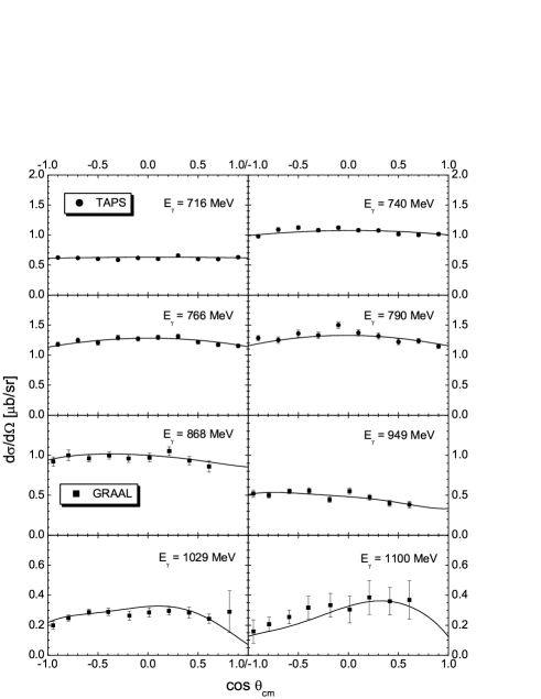
Figure 3: Differential cross section for $\gamma p\rightarrow\eta p$. The data are from TAPS [15] and GRAAL [29].

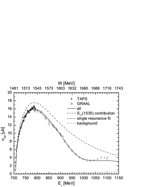
Figure 4: Total cross section for $\gamma p\rightarrow\eta p$. The data are from TAPS [15] and GRAAL [29].

Our results for the total cross section is shown in Fig. 4, and compared with the TAPS and GRAAL data. Again, these are in good agreement except for the bump observed in the GRAAL data in the region $E_{\gamma}^{\mathrm{lab}}$ = 1050 - 1100 MeV that can not be reproduced in our model. However, note that the total cross section of the GRAAL data is obtained from integrating the differential cross sections, by use of a polynomial fit in $\cos\theta$ for extrapolation to the uncovered region. Therefore, the proper way to figure out the discrepancy is to compare the differential cross sections directly. In Fig. 5, we plot the differential cross sections at four different energies between $E_{\gamma}^{\mathrm{lab}}$ = 1050 - 1100 MeV where the bump occurs. It is seen from these differential cross sections that there are no obvious differences, except for the forward angles, where the error bars are quite big. Therefore, we conclude that the discrepancy is due to the extrapolation of the GRAAL data to the forward angles and not heavily supported by the data themselves.

Figure 5: Differential cross section for $\gamma p\rightarrow\eta p$ at energies between $E_{\gamma}^{\mathrm{lab}}$ = 1050 - 1100 MeV. The data are from GRAAL [29].

Table 5: Parameters of the $S_{11}(1535)$ resonance. The results of the single resonance fit are obtained by performing the fit to low energy data using only one $S_{11}$ resonance. The second row is the our full result including two $S_{11}$ resonances.

Fit	Mass	Width	$A^{p}_{1/2}$	$\beta_{\eta N}^{S_{11}(1535)}$
	[MeV]	[MeV]	[$10^{-3}\ \mbox{GeV}^{-1/2}$]
Single $S_{11}$ resonance fit	1536	159	103	$50\%$
Double $S_{11}$ resonance fit	1541	191	118	$50\%$

Fig. 4 shows that the background contribution is very small, and the total cross section is dominated by the $S_{11}(1535)$ at low energy. However, the contribution from the second resonance, $S_{11}(1650)$, can not be neglected. Even though a single $S_{11}$ resonance can fit the low energy data nicely up to $E_{\gamma}^{\mathrm{lab}}$ = 910 MeV (the dash-dotted curve in Fig. 4), it can by no means describe the higher energy region. Moreover, the single resonance fit yields incorrect resonance parameters, as shown in Table 5. In fact, the decay width and photon coupling obtained in the single $S_{11}$ resonance fit are significantly smaller than the full results when both $S_{11}$ resonances are properly included.

4.3 Polarization observables

One special feature in the polarization measurements of $\eta$ photoproduction is that one can access small contributions from a particular resonance through the interference of the dominant $E_{0+}$ multipole with smaller multipoles. For example, if we assume the $s$-wave dominance, the polarized beam asymmetry can be expressed as

$$\Sigma=3\,\sin^{2}\theta\;\mathrm{Re}[E_{0+}^{*}(E_{2-}+M_{2-})]\,/\,|E_{0+}|^{2}\,,$$ (32)

which only depends on the interference of $E_{0+}$ and $(E_{2-}+M_{2-})$ multipoles. Since the background is very small in this reaction, the main source producing $E_{2-}$ and $M_{2-}$ at low energy is the $D_{13}$(1520) resonance. This is the reason why the photon asymmetry is so sensitive to the $D_{13}$(1520) at low energies, and why even the tiny branching ratio can be determined.

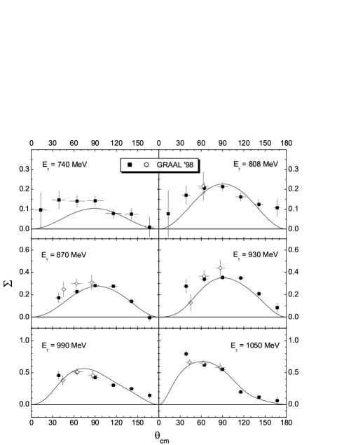
Figure 6: Beam asymmetry for $\gamma p\rightarrow\eta p$. The data are from GRAAL [30].

The available beam asymmetry data were measured at GRAAL [30] from threshold to $E_{\gamma}^{\mathrm{lab}}$ = 1.1 GeV. Higher energy data up to $E_{\gamma}^{\mathrm{lab}}$ = 1.5 GeV are being analyzed and will be available soon [44]. In Fig. 6, we compare our results with these data. An overall good agreement has been achieved. At low energies, we observe that the beam asymmetry has a clear $\sin^{2}\theta$ dependence, which behaves according to Eq. (32) as a result of interference between $s$- and $d$-waves. At the lowest energy (740 MeV) the data show an asymmetric forward-backward (f-b) shape which can not be described with our model. In fact, due to the large suppression of high partial waves this would be true for any model. From these low energy data, a branching ratio of $\beta_{\eta N}=(0.06\pm 0.003)\%$ can be determined for the $D_{13}$(1520). When energies get higher than $E_{\gamma}^{\mathrm{lab}}$ = 930 MeV, the data develop a f-b asymmetry behavior, which becomes especially evident at $E_{\gamma}^{\mathrm{lab}}$ = 1050 MeV. This f-b asymmetry in $\Sigma$ is very sensitive to the $F_{15}$(1680) as discussed by Tiator et al. [23], which is the reason why such a small branching ratio $(0.06\pm 0.02)\%$ can be extracted for this resonance. The same f-b asymmetry behavior is also responsible for the large branching ratio of the $D_{15}$(1675) (17%) in our fit.

Figure 7: Target asymmetry for $\gamma p\rightarrow\eta p$. The data are from Bonn [42].

The target asymmetry for $\gamma p\rightarrow\eta p$ has been measured at Bonn [42] from threshold to $E_{\gamma}^{\mathrm{lab}}$ = 1150 MeV. However, these data are not included in our current fitting because so far all theoretical efforts fail to reproduce them. Instead, we plot the prediction from our model in Fig. 7 and compare with the Bonn data. At low energies, a nodal structure with sign changes at around $90^{\circ}$ is observed from these Bonn data, but is not present in our result. At higher energies, our results for the target asymmetry show an enhancement at forward angles, mainly due to the contribution from the $D_{15}(1675)$. The discrepancy at low energies also occurs in other models [3, 6, 43, 12], and has been discussed in detail in Ref. [23], where it was pointed out that an unexpectedly large relative phase difference between $s$- and $d$-waves is required to explain these Bonn data. Such target asymmetry results, especially the nodal structure at low energies, need to be confirmed by further experiments, and such experiments have been proposed at GRAAL and MAMI. These target asymmetry results should reveal further properties of less-established resonances, as has been already demonstrated by the beam asymmetry results.

Figure 8: Influence of resonances on the differential cross section, the single-polarization observables $\Sigma$, $T$ and $P$, and the double-polarization (beam-target) observables $E$, $F$, $G$, $H$ at a center-of-mass energy $W=1530$ MeV. The solid line is the full isobar model result. The dashed line is obtained without the contributions from the $P_{11}(1710)$, the dotted line without the $D_{15}(1675)$, and the dash-dotted line without both $D_{13}(1520)$ and $D_{13}(1700)$.

Figure 9: Influence of resonances on the differential cross section and polarization observables at a center-of-mass energy $W=1700$ MeV. Notation of the curves as in Fig. 8.

In Figs. 8 and 9 we show two different energy sets of 8 out of 16 possible polarization observables for photoproduction which are currently under consideration. All of them can be reached with a polarized target and linearly or circularly polarized photons. Even the recoil polarization $P$ can be obtained with a polarized target using double polarization. At $W=1530\;\mbox{MeV}$, in the center of the $S_{11}(1535)$ and $D_{13}(1520)$ resonances, the behavior is very strongly dominated by the large $s$-wave $E_{0+}$. As can be seen in Fig. 10,

Figure 10: Real and imaginary parts of $E_{0+}$, $M_{1-}$, $E_{2+}$ and $M_{2+}$ multipoles and $A_{2-}=(3M_{2-}-E_{2-})/2$, $B_{2-}=M_{2-}+E_{2-}$, $A_{3-}=2M_{3-}-E_{3-}$ and $B_{3-}=M_{3-}+E_{3-}$ helicity amplitudes (in $10^{-3}/m_{\pi^{+}}$) for the reaction $\gamma p\rightarrow\eta p$. The nucleon resonances $S_{11}(1535)$, $S_{11}(1650)$, $P_{11}(1710)$, $D_{13}(1520)$, $D_{13}(1700)$, $D_{15}(1675)$ and $F_{15}(1680)$ are indicated by crosses at their mass positions in the corresponding partial channels.

in this region the $s$-wave dominates by even more than a magnitude and for the $p$- and $d$-waves the only sizeable contribution arises from the $B_{2-}$ multipole, the helicity $3/2$ component of the $D_{13}(1520)$ resonance excitation amplitude. Consequently, the differential cross section is practically constant and the helicity asymmetry $E(\theta)$ is unity. In this energy domain $E(\theta)$ can well be used for calibration purposes of circularly polarized photons as this result is highly model independent. For a pure $s$-wave all other polarization observables in Fig. 8 would completely vanish and the values obtained are interferences between the $s$-wave and other resonance and background contributions, where all of them are relatively small. The photon asymmetry $\Sigma$ and the double polarization observable $F$ are strongly dominated by the $s$-$d$ interference $\mbox{Re}[E_{0+}^{*}B_{2-}]$ while all other resonance contributions are negligible. A special case is the target polarization $T$ which is proportional to $\mbox{Im}[E_{0+}^{*}B_{2-}]$. However, as the two resonances are so close together (within 10-20 MeV), the imaginary part disappears in our isobar model. As discussed before, this observable should be of very high priority for a next generation of eta photoproduction experiments. The higher resonances $D_{15}(1675)$, $D_{13}(1700)$ and $P_{11}(1710)$ do not significantly contribute at this low energy, giving the possibility to study the background amplitudes in the target and recoil polarizations $T$ and $P$. The situation changes dramatically in Fig. 9 at $W=1700\;\mbox{MeV}$. The $s$-wave no longer dominates so strongly (see Fig. 10) and higher resonances play bigger roles. The cross section and $E(\theta)$ exhibit structures, the $D_{15}(1675)$ is mostly responsible for the angular shape of the cross section. It also plays a big role in the $\Sigma$, $T$ and $F$ observable. As in the case of pion production, it is generally very difficult to find enhanced sensitivity to $P_{11}$ resonances, like the Roper. In most observables the influence of the $M_{1-}$ multipole is very small. Here in Fig. 9 the recoil polarization and the double polarization observable $H$ give access to study the $P_{11}(1710)$ resonance.

In Fig. 10 the most important partial waves are shown as real and imaginary parts of electric and magnetic multipoles or as helicity 1/2 and 3/2 amplitudes. The $D_{13}(1520)$ and $F_{15}(1680)$ resonances are the two most prominent states with large $A_{3/2}$ photon couplings at $Q^{2}=0$. This can be very well seen in the $B_{2-}$ and $B_{3-}$ amplitudes. On the other hand, the $D_{15}(1675)$ has similar $A_{1/2}$ and $A_{3/2}$ couplings (see Table 4) but is very strongly dominated by magnetic transitions. The fact that in general the real parts of the amplitudes do not vanish at the resonance positions as expected from the Breit-Wigner forms shows the influence of the background contributions.

4.4 Electroproduction results

There are two recent $\eta$ electroproduction data sets from Jefferson Lab: Armstrong et al. [31] measured the $ep\rightarrow e^{\prime}p\eta$ process at high momentum transfer ($Q^{2}=2.4,\,3.6\;(\mbox{GeV/c})^{2}$) and $W$ around the $S_{11}(1535)$ region, while the CLAS collaboration [32] measured at various $Q^{2}$ ($=0.25-1.5\;(\mbox{GeV/c})^{2}$) over a wider energy region ($W=1.5-1.86\;\mbox{GeV}$). When fitting these electroproduction data, we fix all the parameters determined from the photoproduction data except for the $Q^{2}$ dependence of the helicity amplitudes $A^{p}_{1/2,\,3/2}(Q^{2})$. The $Q^{2}$ dependence of the $S_{11}(1535)$ is described by the form of Eq. (29), and the parameters $s_{n}$ and $s_{d}$ are determined from electroproduction data. Fitting all the JLab data, we obtain the results: $s_{n}=2.394\;(\mbox{GeV/c})^{-2}$ and $s_{d}=0.085\;(\mbox{GeV/c})^{-2}$.

In Fig. 11 we plot our total cross section results for the $ep\rightarrow e^{\prime}p\eta$ process at various $Q^{2}$ and compare to the CLAS integrated cross section data [32]. The overall agreement is good, however we notice some deviations in the resonance peak position. Indeed, the value of the $S_{11}(1535)$ mass extracted by the CLAS collaboration is 1519 MeV, while 1541 MeV is obtained from our photoproduction fit. We choose not to change our photoproduction fit value for these electroproduction data.

Figure 11: Total cross section for $p\,(e,e^{\prime}p)\,\eta$ at various $Q^{2}$ compared to the CLAS integrated cross section data [32].

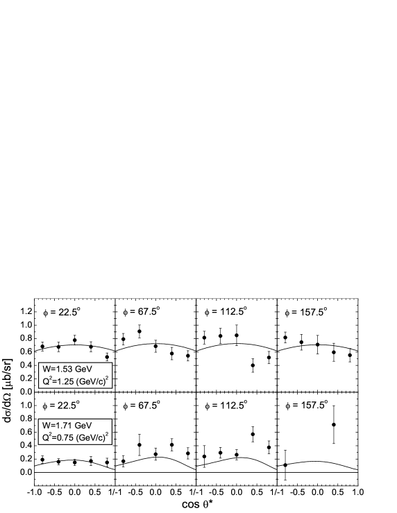
Figure 12: Differential cross section for $p\,(e,e^{\prime}p)\,\eta$ at various $Q^{2}$ compared to the CLAS data [32].

The results for the differential cross sections are shown and compared with the CLAS data in Fig. 12. Discrepancies can be seen at some data points. However, because the statistics of these data is not very good, our results are still within reasonable error regions of these CLAS data. More $\eta$ electroproduction data from CLAS are being analyzed and should be available with better statistics in the near future.

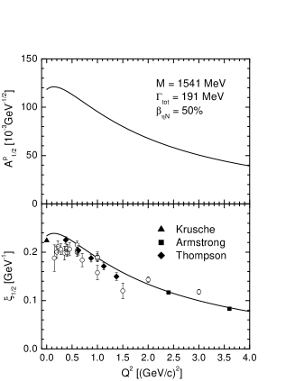
Figure 13: Upper panel: Our results for the photon helicity amplitude $A^{p}_{1/2}(Q^{2})$ for $S_{11}(1535)\rightarrow\gamma p$. Lower panel: The result for the quantity $\xi_{1/2}$ defined in Eq. (33), compared with the values extracted from recent JLab data, Armstrong et al. [31] and Thompson et al. [32], and previous data from Ref. [45]. The photoproduction data point ($Q^{2}=0$) is from Krusche et al. [15].

In Fig. 13 we show our result for the $Q^{2}$ dependence of the photo-excitation helicity amplitude $A^{p}_{1/2}(Q^{2})$ for $S_{11}(1535)\rightarrow\gamma p$. The form of the $Q^{2}$ dependence has been described in Eq. (29). In order to avoid large model uncertainties arising from different values of partial and total widths of the $S_{11}(1535)$ employed in other analyses, we choose not to compare with the helicity amplitudes $A^{p}_{1/2}(Q^{2})$ extracted from other analyses. Instead, we compare the nearly model-independent quantity introduced by Benmerrouche et al. [5],

$$\xi_{\lambda}=\sqrt{\frac{m_{N}k_{R}}{M_{R}q_{R}}\frac{\beta_{\eta N}}{\Gamma_{tot}}}\,A_{\lambda}\,,\qquad\mbox{for $\lambda$ = 1/2, 3/2}\,.$$ (33)

As opposed to the uncertainty from $\beta_{\eta N}$ and $\Gamma_{tot}$ between different analyses, the quantity $\xi_{\lambda}$ is almost independent of the extraction process. In Fig. 13 we compare our $\xi_{1/2}(Q^{2})$ values for $S_{11}(1535)$ with the ones extracted from the recent JLab data [31, 32] and older data [45]. It is seen that overall good agreement is achieved up to $Q^{2}=4.0\;\mbox{(GeV/c)}^{2}$.

5 Summary and Conclusions

In this work we have presented a new study of eta photo- and electroproduction in an isobar model. The model has been developed similarly to the unitary isobar model MAID for pion electroproduction. It is based on nucleon Born terms, vector meson exchange contributions in the $t$-channel and $s$-channel nucleon resonance excitations described as in MAID by Breit-Wigner shapes. This allows a direct comparison between our pion and eta production analyses. Based on experimental data from Mainz, GRAAL and JLab we have obtained a very good fit of photo- and electroproduction cross sections and photon asymmetries. We find significant contributions of the $D_{13}(1520)$, $S_{11}(1535)$, $S_{11}(1650)$, $D_{15}(1675)$, $F_{15}(1680)$, $D_{13}(1700)$, $P_{11}(1710)$ and $P_{13}(1720)$ resonances. Generally the resonance decay widths, the branching ratios and the e.m. helicity couplings are strongly correlated, and in a photo- or electroproduction experiment only the combined quantity $\xi$ (see Eq. (33)) can be uniquely determined. For the $S_{11}(1535)$ the $\eta N$ branching ratio is rather well known from $(\pi,\eta)$ reactions, giving us the possibility to concentrate our studies on the photon coupling $A_{1/2}$. Our result of $118\times 10^{-3}\;\mbox{GeV}^{-1/2}$ is in good agreement with previous detailed studies [15, 21]. However, we find a big influence of the second $S_{11}(1650)$ that is absolutely necessary to describe the total cross sections at energies above $W=1600\;\mbox{MeV}$. Fitting also electroproduction data of JLab allowed us to further determine the $Q^{2}$ evolution of $A_{1/2}(Q^{2})$ with a simple parameterization. Our result confirms the $Q^{2}$ points of the experimental analyses and yields a form factor that falls off much more slowly than the nucleon dipole form factor or the $N\rightarrow\Delta(1232)$ transition form factor.

For the higher resonances we find large branching ratios of $7.9\%$, $17\%$ and $26\%$ for $S_{11}(1650)$, $D_{15}(1675)$ and $P_{11}(1710)$, respectively, but very small values of only $0.06\%$ for the $D_{13}(1520)$ and $F_{15}(1680)$. A remarkable result is obtained for the $E/M$ ratio of the $D_{15}(1675)$ that turns out to be only $1.4\%$ (PDG gives $20\pm 27\%)$. This ratio can be expressed as $(A_{1/2}-\frac{1}{\sqrt{2}}A_{3/2})/(A_{1/2}+\sqrt{2}A_{3/2})$ and would be expected to approach $100\%$ from helicity conservation at large $Q^{2}$ as in the case of the $N\rightarrow\Delta(1232)$ excitation. An investigation of this interesting ratio will be possible by an electroproduction experiment with $R_{TT}$ separation.

Concerning the background processes our fits confirm a very small $\eta NN$ coupling constant of $g_{\eta NN}^{2}/4\pi=0.10$ with a slight preference for a pseudoscalar coupling. However, as the coupling strength weakens, this preference finally diminishes. We have also looked for a possible “missing” $S_{11}$ resonance in the region around 1700 MeV. However, in our isobar model such an additional state is not supported by the fits to the data.

Finally, the only data that we can not sufficiently describe are the target polarization data in the threshold region. As already found in the model independent analysis of Ref. [23], the structure found in the target polarization goes beyond the scope of an isobar model and would require a very large “background” from another mechanism, not considered in our model, nor in any other model so far. Further measurements of this and other target polarization observables with double polarization would be very useful to track down the underlying mechanism of the threshold $s$-wave production if it should not be given by the $S_{11}(1535)$ resonance alone.

References

- [1] C. Bennhold and H. Tanabe, Nucl. Phys. A530 (1991) 625.
- [2] C. Sauermann, B.L. Friman and W. Nörenberg, Phys. Lett. B341 (1995) 261.
- [3] T. Feuster and U. Mosel, Phys. Rev. C59 (1999) 460.
- [4] A. Waluyo et al., Proceedings of the Workshop on the Physics of Excited Nucleons (NSTAR 2001), Mainz, Germany, eds. D. Drechsel and L. Tiator (World Scientific, Singapore, 2001).
- [5] M. Benmerrouche, N.C. Mukhopadhyay and J.F. Zhang, Phys. Rev. D51 (1995) 3237.
- [6] N.C. Mukhopadhyay and N. Mathur, Phys. Lett. B444 (1998) 7.
- [7] R.M. Davidson, N. Mathur and N.C. Mukhopadhyay, Phys. Rev. C62 (2000) 058201.
- [8] B. Borasoy, Eur. Phys. J. A9 (2000) 95.
- [9] B. Borasoy, Phys. Rev. D63 (2000) 094015.
- [10] Z. Li, Phys. Rev. C52 (1995) 1648.
- [11] Z. Li, H. Ye and M. Lu, Phys. Rev. C56 (1997) 1099.
- [12] B. Saghai and Z. Li, Eur. Phys. J. A11 (2001) 217.
- [13] G. Knöchlein, D. Drechsel and L. Tiator, Z. Phys. A352 (1995) 327.
- [14] B. Schoch et al., Prog. Part. Nucl. Phys. 34 (1995) 43.
- [15] B. Krusche et al., Phys. Rev. Lett. 74 (1995) 3736.
- [16] J. Denschlag, L. Tiator and D. Drechsel, Eur. Phys. J. A3 (1998) 171.
- [17] G. Höhler and A. Schulte, Newslett. 7 (1992) 94.
- [18] G. Höhler, Newslett. 9 (1993) 1.
- [19] D.E. Groom et al., Eur. Phys. J. C15 (2000) 1.
- [20] R. Koniuk and N. Isgur, Phys. Rev. D21 (1980) 1868.
- [21] B. Krusche et al., Phys. Lett. B397 (1997) 171.
- [22] F. Ritz and H. Arenhövel, Phys. Rev. C64 (2001) 034005.
- [23] L. Tiator, D. Drechsel, G. Knöchlein, and C. Bennhold, Phys. Rev. C60 (1999) 035210.
- [24] R. Workman, R.A. Arndt and I.I. Strakovsky, Phys. Rev. C62 (2000) 048201.
- [25] L. Tiator, C. Bennhold and S.S. Kamalov, Nucl. Phys. A580 (1994) 455.
- [26] M. Kirchbach and L. Tiator, Nucl. Phys. A604 (1996) 385.
- [27] S. Neumeier and M. Kirchbach, Int. J. Mod. Phys. A15 (2000) 4325.
- [28] D. Drechsel, O. Hanstein, S.S. Kamalov, and L. Tiator, Nucl. Phys. A645 (1999) 145.
- [29] F. Renard et al., hep-ex/0011098.
- [30] J. Ajaka et al., Phys. Rev. Lett. 81 (1998) 1797.
- [31] C.S. Armstrong et al., Phys. Rev. D60 (1999) 052004.
- [32] R. Thompson et al., Phys. Rev. Lett. 86 (2001) 1702.
- [33] J.D. Bjorken and S.D. Drell, Relativistic Quantum Mechanics, McGraw-Hill, New York, 1964.
- [34] A. Donnachie and G. Shaw, Electromagnetic Interactions of Hadrons, New York, 1978.
- [35] E. Amaldi, S. Fubini and G. Furlan, Pion-Electroproduction, Springer-Verlag, Berlin, 1979.
- [36] D. Drechsel and L. Tiator, J. Phys. G18 (1992) 449.
- [37] W.-T. Chiang and F. Tabakin, Phys. Rev. C55 (1997) 2054.
- [38] R.L. Walker, Phys. Rev. 182 (1969) 1729.
- [39] R.M. Davidson, N.C. Mukhopadhyay and R.S. Wittman, Phys. Rev. D43 (1991) 71.
- [40] O. Dumbrajs et al., Nucl. Phys. B216 (1983) 277.
- [41] V. Burkert and Zh. Li, CEBAF proposal PR-92-017 (1992).
- [42] A. Bock et al., Phys. Rev. Lett. 81 (1998) 534.
- [43] Z. Li and B. Saghai, Nucl. Phys. A644 (1998) 345.
- [44] A. D’Angelo (for the GRAAL Collaboration), Proceedings of the Workshop on the Physics of Excited Nucleons (NSTAR 2001), Mainz, Germany, eds. D. Drechsel and L. Tiator (World Scientific, Singapore, 2001).
- [45] F.W. Brasse et al., Nucl. Phys. B139 (1978) 37; F.W. Brasse et al., Z. Phys. C22 (1984) 33; U. Beck et al., Phys. Lett. B51 (1974) 103; H. Breuker et al., Phys. Lett. B74 (1978) 409.