Constraints on proton-proton fusion from helioseismology

Abstract

The proton-proton ($pp$) fusion cross-section found at the heart of solar models is unconstrained experimentally and relies solely on theoretical calculations. Effective field theory provides an opportunity to constrain the $pp$ cross-section experimentally, however, this method is complicated by the appearance of two-nucleon effects in the form of an unknown parameter $L_{1,A}$. We present a method to constrain $L_{1,A}$ using the Standard Solar Model and helioseismology. Using this method, we determine a value of $L_{1,A}$ = 7.0 fm³ with a range of 1.6 to 12.4 fm³. These results are consistent with theoretical estimates of $L_{1,A}\approx$ 6 fm³.

I Introduction

The Standard Solar Model (SSM) is a model of the sun constructed by numerically solving the equations of stellar structure and evolution constrained by the observed composition, luminosity, and radius of the sun at the current age. This model yields acoustic oscillation frequencies ($p$-modes) that match the observed $p$-mode oscillation spectrum of the sun to better than 0.3% Gue97 . The uncertainties associated with the observed oscillation frequencies are an order of magnitude smaller. The excellent agreement between the model and observed frequency spectra implies that the run of sound speed predicted by the model is close to that of the sun which, in turn, suggests that the physics used to construct the model of the sun is accurate.

The individual $p$-mode frequencies extend to distinct depths in the sun, and hence can be used to study the physics of specific regions. Of interest to the work described here are the low-$l$ (where $l$ corresponds, in spherical harmonic nomenclature, to the number of nodes in azimuth) $p$-mode frequencies that penetrate deep into the core of the sun. These modes, grouped in combinations that cancel out surface dependencies, can be used to test the important physics of the core. One of the greatest sources of uncertainty in the physics of the solar model core is the $pp$-fusion cross-section. The reaction is unconstrained by laboratory-based experiments, relying completely on precise calculations from theoretical nuclear physics. Owing to the precise agreement between the observed and predicted oscillation frequencies that already exists, it is possible to use the oscillation frequencies to constrain the $pp$ cross-section, that is, to determine the range of cross-sections that yield oscillation frequencies within the known uncertainties of the solar model physics and constraints. To date, this sort of constraint has been imposed only through simplifications of the standard solar model antia , and here we use a fully-developed stellar evolution code, to be discussed later.

The cross-section for $pp\rightarrow de^{+}\nu_{e}$ has been studied extensively Sal52 ; Bli65 ; Bah69 ; Gar72 ; Dau76 ; Bar79 ; Gou90 ; Car91 ; Kam94 ; Iva97 ; Sch98 ; Par98 and contains two components. First, an ‘Impulse Approximation’ (IA) contribution where the weak interaction takes place on a single proton, as shown in Fig. 1a). This comprises more than 95% of the cross-section at energies of solar interest and is very well understood because it concerns only the weak properties of a proton and well-known proton-proton scattering physics. The second component, and the remainder of the cross-section, is unconstrained by experiment and has led theorists to try to improve our understanding of this process. Conventional potential model calculations will introduce so-called meson-exchange currents; essentially two-nucleon effects where the weak interaction occurs while the two nucleons are interacting with each other. An example of such a process is shown in Fig. 1b). These two-nucleon effects introduce physics that cannot be constrained directly by $pp$ elastic scattering experiments, and the parameters of this extended physics must be constrained using other methods. Few other methods exist.

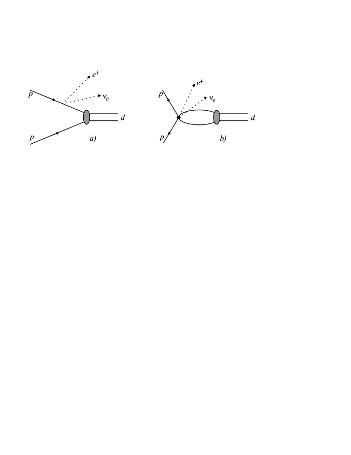
Figure 1: The process $pp\rightarrow de^{+}\nu_{e}$. a) The Impulse Approximation (IA), where the weak interaction takes place on one proton while the other proton is just a spectator. The final state, represented by the grey bubble, is the resulting neutron and proton being bound as a deuteron. b) A two-nucleon process where the protons are undergoing a strong interaction at the same time as the weak interaction (represented by the black circle).

Neutrino-deuteron scattering could, in principle, constrain the two-nucleon effects. Experiments involving neutrino-deuteron scattering are, however, quite difficult. Reactor antineutrino-deuteron experiments can be performed, where the experimental uncertainties are of order 10-20%. Nonetheless, they can be used to infer a constraint on the two-nucleon matrix elements bcv . One interesting method is to use tritium $\beta$-decay to constrain the two-nucleon matrix elements needed in $pp\rightarrow de^{+}\nu_{e}$ Sch98 . The tritium half-life is well known, and the same two-nucleon effects occur here as in $pp$ fusion. However, there are three nucleons in tritium, hence we cannot be certain that this more complicated structure does not, in turn, complicate the weak interaction physics further.

If we were to rely purely on theory to predict the two-nucleon component of the $pp$ fusion cross-section, we still have one more problem. How do we define the uncertainty in a theoretical calculation? In quantum field theories, such as quantum electrodynamics, there is a perturbative expansion parameter that dictates the size of contributions at each order in perturbation theory and thus the size of any neglected remainder. The remainder represents the uncertainty in the theory. However, conventional nuclear physics calculations use Schrödinger’s equation and nucleon-nucleon potentials to calculate initial and final-state wavefunctions and, in turn, calculate the matrix elements of relevant transition operators. In this approach, no scheme exists for estimating the size of contributions from unknown or neglected physics. An alternative to using wavefunctions to study our problem is to use an effective field theory (EFT). An EFT has many benefits, but there are drawbacks. If the EFT is perturbative (i.e., there is a small expansion parameter), then one can compute to a specific order in the parameter and then make direct statements of the scale of theoretical uncertainty of the problem as determined by the relative size of the next term in the expansion - just as one would do in quantum electrodynamics. This is particularly important given that EFTs typically have an infinite number of terms, and the expansion parameter is required to ensure that only a finite number of terms are needed for any given calculation. In the particular case of nuclear EFTs, specifically ones where all interactions are of zero-range (i.e., no pions), the expansion parameter is denoted by $\epsilon=Q/M_{\pi}$, where $Q$ represents a generic momentum in the problem and $M_{\pi}$ is the pion mass. An added benefit of this approach is that field theories pose no problems for conservation laws such as electromagnetic gauge invariance, which are often difficult to preserve when wavefunctions are used. However, EFTs cannot escape the problem that all parameters in an EFT must be constrained by experiment, including the various weak interaction parameters.

II Proton-Proton Fusion

There have been a number of works dealing with $pp$-fusion in EFT KRpp ; KRem ; BC , using the EFT without pions developed in refs. KSW96 ; K97 ; vK97 ; Cohen97 ; BHvK1 ; crs . As with the traditional calculations, the strength of the weak interaction on an interacting pair of nucleons is unknown and this ignorance can be specified through one parameter, which we label $L_{1,A}$ BC . $L_{1,A}$ represents the strength of the interaction shown in Fig. 1b). It also appears in the various $\nu(\overline{\nu})-d$ breakup reactions and a precise measurement of one of those reactions would also constrain $pp$-fusion. However, precise measurements do not exist (but have been proposed ORLaND ).

It is also interesting to consider the inverse of this argument. A constraint on $pp$-fusion would lead to a constraint on $\nu(\overline{\nu})-d$ breakup reactions. The recent results from the Sudbury Neutrino Observatory (SNO) SNO1 ; SNO2 rely on the reaction $\nu_{e}d\rightarrow e^{-}pp$ to detect and extract the solar neutrino flux, hence the theoretical uncertainties in the cross-section certainly affect their results. In spite of the importance of SNO, not as much attention has been paid to these breakup reactions, particularly the pair

$$\nu_{e}d \rightarrow e^{-}pp\>,$$ (1)

$$\nu_{x}d \rightarrow\nu_{x}pn\>.$$ (2)

The first reaction commonly known as the Charged-Current (CC) reaction, is sensitive to the electron neutrino ($\nu_{e}$) flux only. The second Neutral-Current (NC) reaction is equally sensitive to electron, muon, and tau neutrinos (denoted by $\nu_{x}$), and provides the key test for neutrino oscillations. The CC reaction is very closely related to $pp$-fusion, but the finite energy/momentum transfers in the CC and NC reactions make conventional calculations much more difficult than the (relatively) simpler $pp$-fusion calculation. However, both $pp$-fusion and deuteron breakup can be calculated using the same EFT in a straightforward manner and the connection between the two is discussed elsewhere BC . Here, we wish to explore the possibility of using the high-precision associated with helioseismology to impose some additional constraints on $L_{1,A}$. In turn, the implications of these constraints can be seen for $\nu-d$ breakup and for SNO.

Cross-sections of astrophysical interest are written as

$$\sigma(E)={S(E)\over E}\exp(-2\pi\eta)\>,$$ (3)

separating the nuclear physics ($S(E)$) from the longer range Coulomb effects (the Gamow factor $\exp(-2\pi\eta)$). In the particular case of $pp$-fusion, we are interested in $S_{pp}(0)$. Adelberger et al. Ade98 parameterize $S_{pp}(0)$ as

$$S_{pp}(0)=4.00\times 10^{-25}{\rm MeV\,b}\bigg{(}{(ft)_{0^{+}\rightarrow 0^{+}}\over 3073\ {\rm s}}\bigg{)}^{-1}\bigg{(}{\Lambda^{2}\over 6.92}\bigg{)}\bigg{(}{g_{A}/g_{V}\over 1.2654}\bigg{)}^{2}\bigg{(}{f_{pp}^{R}\over 0.144}\bigg{)}\bigg{(}{1+\delta\over 1.01}\bigg{)}^{2}$$ (4)

where the parameters are described in ref. Ade98 . Of importance here are $\Lambda$ and $\delta$. Their parameterization uses an explicit separation of IA and two-nucleon effects into $\Lambda$ and $\delta$ respectively. In this separation the total matrix element for the fusion process is given by $\Lambda(1+\delta)$. This separation is artificial and is not appropriate when a fully self-consistent nuclear physics calculation is performed. Consequently, we set $\delta=0$ and incorporate all effects directly into $\Lambda$.

In EFT, it was found that BC

$$\Lambda=2.58+0.011\left(\frac{L_{1,A}}{\text{1 fm}^{3}}\right)-0.0003\left(\frac{K_{1,A}}{\text{1 fm}^{5}}\right)\ .$$ (5)

where $L_{1,A}$ parameterizes two-nucleon physics at next-to-leading order (NLO), and $K_{1,A}$ parameterizes two-nucleon physics at next-to-next-to-next-to-leading order (NNNLO). No new parameters appear at the intermediate order (NNLO). Naively, each order of the expansion will be (naively) 30% of the previous order. So, a calculation to N⁴LO should have a precision of 1%. In practice, low-energy calculations of this type are usually more rapidly convergent. $L_{1,A}$ and $K_{1,A}$ are both unknown, and need to be constrained experimentally. Dimensional analysis as developed in refs. crs ; KSW favors

$$\left|L_{1,A}\right| \approx \frac{1}{m_{\pi}\left(m_{\pi}-\gamma\right)^{2}}\approx 6\text{ fm}^{3}\ ,$$

$$\left|K_{1,A}\right| \approx \frac{1}{m_{\pi}^{2}\left(m_{\pi}-\gamma\right)^{3}}\approx 20\text{ fm}^{5}\ .$$ (6)

It can be shown that $K_{1,A}$ would contribute at an order much less than 1%, so we neglect it BC .

III Helioseismology and the Standard Solar Model

The solar models for this investigation were constructed using the Yale stellar evolution code (YREC) in its non-rotating configuration Gue97 ; Pin88 ; Gue92 . The code implements the most current constitutive physics available. The equation of state tables are provided by the OPAL group Rog86 ; Rog96 . The opacities in the interior are interpolated from the OPAL opacity tables Igl96 , and the lower temperature opacities, near the surface, are interpolated from the Alexander and Ferguson Alx94 tables.

The nuclear reaction cross-sections have recently been updated (compared to Gue97 ) to correspond to the latest agreed upon values set at the 1998 Seattle Workshop on Solar Fusion Reactions. The nuclear energy generation routines are nearly identical to those used by Bahcall et al. Bah95 who, themselves, use a variation of YREC for their solar model calculations. To facilitate quick adjustments of S-factors for each reaction, YREC uses Bahcall Bah89 values multiplied by a scaling factor $S(0)/S^{*}(0)$, where $S(0)$ is the revised S-factor, and $S^{*}(0)$ is the original Bahcall value Bah89 . For the results presented in this investigation, we adjust the scaling factor corresponding to the $pp\rightarrow de^{+}\nu_{e}$ reaction. The models were evolved from the zero age main sequence (ZAMS, the point in the evolution of the star where the nuclear power first dominates gravitational power) in 100 equally spaced time steps to 4.55 Gyr. The meteoritic age of the Sun, that is the age implied from the age of the oldest meteorites, is 4.52$\pm$0.04 Gyr Gue89 . Here we use 4.55 Gyr for the age of the solar model, which lies within the uncertainty range of the meteoritic age, to facilitate testing and comparison of our models to solar models that we and others have calculated in the past. The solar radius, $R_{\odot}=6.958\times 10^{10}$ cm, and the solar luminosity, $L_{\odot}=3.8515\times 10^{33}$ erg s^-1, are known to better than $\pm$0.05%. The mass of the Sun is $1.989\times 10^{33}$ g with a relative uncertainty of $\pm$0.02% Coh86 . The mixing length parameter, a free parameter in the mixing length theory  used to model convective energy transport, and the helium abundance, an element whose abundance cannot be determined from spectroscopic measurements of the photosphere of the Sun, are adjusted to produce models that match each other and the above-stated values of $R_{\odot}$ and $L_{\odot}$ to one part in $10^{6}$.

In order for the surface composition of the (evolved) solar model to match the observationally determined abundances, we set the initial (ZAMS) homogeneous composition for hydrogen, helium and metals (A$>$4) by mass fraction to 0.70633, 0.27367, and 0.02000, respectively. The effects of gravitational settling of helium and metals, which alters the surface abundances as the models evolve, are modeled using the diffusion formulation described by Bahcall et al. Bah95 . Other modeling details are as described in Gue97 .

To constrain the range for $L_{1,A}$, a relationship between $L_{1,A}$ and $S_{pp}$ is established. Neglecting the higher-order effects of $K_{1,A}$ in eq. 5,

$$\Lambda=2.58+0.011\left(\frac{L_{1,A}}{\text{1 fm}^{3}}\right)\$$ (7)

and applying the appropriate values from Ade98 to eq. 4 gives

$$S_{pp}(0)=0.56663\times 10^{-25}(\Lambda^{2}){\rm MeV\,b}\>.$$ (8)

The combination of eqs. 7 and 8 establishes a relationship between $L_{1,A}$ and $S_{pp}$(0), given by

$$S_{pp}(0)=3.7717\times 10^{-25}\bigg{(}1+8.53\times 10^{-3}\ \bigg{(}{L_{1,A}\over 1\ {\rm fm}^{3}}\bigg{)}+1.82\times 10^{-5}\ \bigg{(}{L_{1,A}\over 1\ {\rm fm}^{3}}\bigg{)}^{2}\bigg{)}\ {\rm MeV\,b}\>.$$ (9)

Using the above relationship and the current theoretical value for $S_{pp}$(0), the best determined value for $L_{1,A}$ may be calculated. By varying the $S_{pp}$(0) value within YREC in accordance with values of $L_{1,A}$, solar models are produced corresponding to each variation.

The resultant models are then read into a nonradial, nonadiabatic stellar oscillation program Gue94 where the oscillation frequencies are calculated. We adopt the usual nomenclature describing different orders of acoustic oscillations, or $p$-modes, with the radial order of the mode given by $n$ and the azimuthal order of the mode given by $l$. Only the lowest $l$-valued $p$-modes (i.e., $l=0,1$) penetrate into the central nuclear burning regions of the sun. The radius to which a mode penetrates, the inner turning point $r_{t}$, is related to the cyclic frequency $\omega$ and the sound speed $c(r_{t})$ by unno

$$r_{t}={\sqrt{l(l+1)}c(r_{t})\over\omega}\>.$$ (10)

This behaviour is shown in Fig. 2.

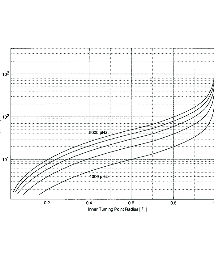
Figure 2: Five curves representing $p$-mode frequencies at 1000 $\mu$Hz, 2000 $\mu$Hz,…, 5000 $\mu$Hz in a plot of the radius fraction of the inner turning point versus azimuthal order. The inner turning point approaches the core as $l$ decreases.

The physics used to model the structure near the surface of the solar model is more uncertain than the physics of the core. Indeed, comparisons of $p$-mode frequencies that probe the surface reveal greater discrepancies between model and observations than in the core. It is believed that the mixing length approximation used to model convection is the principal modeling uncertainty. The frequencies of all observed $p$-modes are affected by this region. It is possible, though, to select pairs of $p$-modes that have identical eigenfunction shape near the surface, and distinct shape in the deep interior, and use them in combination to cancel out the surface layer effects. This is achieved via the small frequency spacing, $\delta\nu(n,l)$, which is defined as the frequency difference between an $\nu(n,l)$ and an $\nu(n-1,l+2)$ $p$-mode. For $l$ = 0 and 1, the $\delta\nu(n,l)$ is well known as one of the most sensitive helioseismic diagnostics of the central-most regions of the Sun.

IV Results

The best value for $L_{1,A}$ is determined by using the current value for $S_{pp}$(0). From Ade98 , the current value for $S_{pp}$(0) is

$$S_{pp}(0)=4.00(1\pm 0.007^{+0.020}_{-0.011})\times 10^{-25}{\rm MeV\,b}$$ (11)

Using eqs. 7 and 11, the determined value for the unknown counterterm is found to be, $L_{1,A}$ = 7.0 fm³.

To determine the range in $L_{1,A}$ using helioseismology, plots of $\delta\nu(n,l)$ versus adiabatic oscillation frequencies are created. To enhance the analysis, $\delta\nu(n,l)$ differences are used instead of $\delta\nu(n,l)$. These differences are formed by taking the $\delta\nu(n,l)$ results from the individual models and subtracting the observed $\delta\nu(n,l)$ for the Sun; $\delta\nu_{model}(n,l)$ - $\delta\nu_{\odot}(n,l)$, where $\delta\nu_{\odot}(n,l)$ values are calculated from observed solar oscillation frequencies.

Low-$l$ small spacings have been published for a number of different high quality solar $p$-mode observations, including GONG (Global Oscillation Network Group; Har96 ; Chr96 ) and BiSON (Birmingham Solar Oscillation Network; Cha99 ). Here we choose the BiSON data set because the uncertainties are low and because we have used this data set before and are familiar with it.

A plot of $\delta\nu(n,l)$ differences versus adiabatic frequencies for the reference SSM is shown in Fig. 3. In Fig. 3, the thick solid line represents the reference SSM model result. The error bars correspond to the uncertainties stated for the observed BiSON results for the Sun Cha99 .

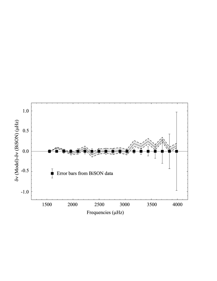
Figure 3: The small spacing frequencies $\delta\nu(n,l)$ for the reference SSM, shown relative to the observed values from BiSON. The error bars represent the uncertainties in the BiSON data. The discrepancies between the model and observations are largest at high frequencies, which are most sensitive to surface effects. The reference SSM uses a value for $L_{1,A}$ of 7.0 fm³, and is shown by a solid black line. The shaded area represents the variation of $L_{1,A}$ between 1.6 and 12.4 fm³.

The low-$l$ small spacing frequencies of our reference SSM lie almost entirely within the uncertainty range of the observationally derived small spacings. This suggests that the interior structure of our model is a very close fit to the actual sun. Which, in turn suggests that the physics specific to this region are accurate, including the age estimate, the chemical abundance and diffusion processes, the opacities, the equation of state, and the nuclear reaction rates. That is, no modifications to the current SSM are required to make it agree with the most accurate $p$-mode data we currently have available to us. It is comforting that the simplest, non-ad-hoc, physics has produced an accurate match to the observed $p$-mode data.

The analysis described above was repeated for each, nonstandard, model corresponding to a variation of $L_{1,A}$ with respect to the reference SSM. A quantitative estimate of the range of $L_{1,A}$ is established by comparing the distribution of the frequency results for various $L_{1,A}$ with respect to the observed BiSON error bars. To extract this quantitative result, the frequency range of $\sim$2500 to $\sim$3000 $\mu$Hz was studied since this frequency range for the SSM showed an excellent fit to the observed BiSON data.

For each model results, average $\delta\nu(n,l)$ difference values were calculated within the frequency range of $\sim$2500 to $\sim$3000 $\mu$Hz. The average observed error within this frequency range was calculated to be $\pm$0.066 $\mu$Hz. Average $\delta\nu(n,l)$ differences are plotted versus the corresponding $L_{1,A}$ value for both the upper and lower range. These plots show a linear relation between the average $\delta\nu(n,l)$ differences and $L_{1,A}$. From this relation and the average observed error values, the values of $L_{1,A}$ corresponding to the upper and lower limits of the error bars are calculated. The upper limit is determined to be 12.4 fm³. The lower limit is determined to be 1.6 fm³. The range of allowed values is shown as the shaded area in Fig. 3. Therefore the value and effective range for $L_{1,A}$ is determined to be

$$L_{1,A}=7.0\pm 5.4\ {\rm fm}^{3}$$ (12)

A further result from the determined SSM is the calculation of the theoretical total ${}^{8}B$ neutrino flux of $4.93\times 10^{6}$ cm^-2s^-1. This result is consistent with the total observed ${}^{8}B$ neutrino flux from SNO of $(5.09^{+0.44}_{-0.43}{\rm(stat)}^{+0.46}_{-0.43}{\rm(syst)})\times 10^{6}$ cm^-2s^-1 SNO2 .

We have tacitly assumed that the uncertainty in the model-computed $p$-mode frequencies is comparable to, or less than, the error bars associated with the observed frequencies. This is not too unreasonable since the model-computed frequencies do lie within the uncertainty error bars of the observations. In order to more formally justify this assumption, we must carry out an extensive uncertainty analysis of the solar model physics and their impact on the computed $p$-mode frequencies. This important task, upon which all similar helioseismic tests depend, is in progress and will be reported at a later time.

V Conclusions

Using the relationship between effective field theory, nuclear cross-sections and the accuracy of helioseismology, the unknown counterterm, $L_{1,A}$, is determined to have a value of 7.0 fm³ with a range of 1.6 to 12.4 fm³. This result for $L_{1,A}$ is consistent with the theoretical value determined by Butler $\&$ Chen BCK using dimensional analysis of $L_{1,A}$ $\approx$ 6 fm³. The result and range is also consistent with other evaluations of $L_{1,A}$ which include 5.6$\pm$2.0 fm³ NSGK and 6.5$\pm$2.4 fm³ Sch98 .

The standard solar model determined for this work shows remarkably excellent agreement with the latest BiSON oscillation frequency observations. Theoretical total fluxes for ${}^{8}B$ neutrinos from the standard solar model result also show excellent agreement with total observed ${}^{8}B$ fluxes reported from the Sudbury Neutrino Observatory.

VI Acknowledgments

The authors would like to thank the Natural Sciences and Engineering Research Council (NSERC) of Canada for its support of this research.

References

- (1) D.B. Guenther and P. Demarque, Astrophys. J. 484, 937 (1997).
- (2) H.M. Antia and S.M. Chitra, Astron. Astrophys. 347, 1000 (1999).
- (3) E.E. Salpeter, Phys. Rev. 88, 547 (1952).
- (4) R.J. Blin-Stoyle and S. Papageorgiou, Nucl. Phys. 64, 1 (1965).
- (5) J.N. Bahcall and R.M. May, Astrophys. J. 152, L17 (1968).
- (6) M. Gari and A.H. Huffman, Astrophys. J. 178, 543 (1972).
- (7) F. Dautry, M. Rho, and D.O. Riska, Nucl. Phys. A264, 507 (1976).
- (8) C. Bargholtz, Astrophys. J. Lett. Ed. 233, 61 (1972).
- (9) R.J. Gould and N. Guessoum, Astrophys. J. 359, L67 (1990).
- (10) J. Carlson, D.O. Riska, R. Schiavilla, and R.B. Wiringa, Phys. Rev. C 44, 619 (1991).
- (11) M. Kamionkowski and J.N. Bahcall, Astrophys. J. 420, 884 (1994).
- (12) A.N. Ivanov, N. I. Troitskaya, M. Faber and H. Oberhummer, Nucl. Phys. A617, 414 (1997); Erratum-ibid. A618, 509 (1997); A.N. Ivanov, H. Oberhummer, N.I. Troitskaya and M. Faber, nucl-th/9910021; Eur. Phys. J. A8, 223 (2000).
- (13) R. Schiavilla et al., Phys. Rev. C 58, 1263 (1998).
- (14) T.-S. Park, K. Kubodera, D.-P. Min, M. Rho, Astrophys. J. 507, 443 (1998).
- (15) M.N. Butler, J.-W. Chen, P. Vogel, nucl-th/0206026, submitted to Phys. Lett. B.
- (16) X. Kong and F. Ravndal, Nucl. Phys. A656, 421 (1999); Nucl. Phys. A665, 137 (2000); Phys. Lett. B470, 1 (1999); Phys. Rev. C 64, 044002 (2001).
- (17) X. Kong and F. Ravndal, Phys. Lett. B450, 320 (1999).
- (18) M.N. Butler and J.-W. Chen, Phys. Lett. B520, 87 (2001 ).
- (19) D.B. Kaplan, M.J. Savage and M.B. Wise, Nucl. Phys. B478, 629 (1996).
- (20) D.B. Kaplan, Nucl. Phys. B494, 471 (1997).
- (21) U. van Kolck, hep-ph/9711222; Nucl. Phys. A645 273 (1999).
- (22) T.D. Cohen, Phys. Rev. C55, 67 (1997); D.R. Phillips and T.D. Cohen, Phys. Lett. B390, 7 (1997); S.R. Beane, T.D. Cohen, and D.R. Phillips, Nucl. Phys. A632, 445 (1998).
- (23) P.F. Bedaque and U. van Kolck, Phys. Lett. B428, 221 (1998).
- (24) J.W. Chen, G. Rupak and M.J. Savage, Nucl. Phys. A653, 386 (1999).
- (25) D.B. Kaplan, M.J. Savage and M.B. Wise, Phys. Lett. B424, 390 (1998); Nucl. Phys. B534, 329 (1998); Phys.Rev. C 59, 617 (1999).
- (26) F.T. Avignone and Yu.V. Efremenko, in Proceedings of the 2000 Carolina Conference on Neutrino Physics, ed. K. Kubodera (World Scientific, 2000) in press.
- (27) Q.R. Ahmad et al. (SNO Collaboration), Phys. Rev. Lett. 87, 071301 (2001).
- (28) Q.R. Ahmad et al. (SNO Collaboration), nucl-ex/0204008.
- (29) E.G. Adelberger et al., Rev. Mod. Phys. 70, 4, 1 265 (1998).
- (30) M.H. Pinsonneault, Ph.D. thesis, Yale University, (1988).
- (31) D.B. Guenther, P. Demarque, Y.-C. Kim and M. Pinsonneault, Astrophys. J. 387, 372 (1992).
- (32) F.J. Rogers, Astrophys. J. 310, 723 (1986).
- (33) F.J. Rogers, F.J. Swenson and C.A. Iglesias, Astrophys. J. 456, 902 (1996).
- (34) C.A. Iglesias and F.J. Rogers, Astrophys. J. 464, 943 (1996).
- (35) D.R. Alexander and J.W. Ferguson, Astrophys. J. 437, 879 (1994).
- (36) J.N. Bahcall, M.H. Pinsonneault and G.J. Wasserburg, Rev. Mod. Phys. 67, 781 (1995).
- (37) J.N. Bahcall, Neutrino Astrophysics, Cambridge University Press: Cambridge, (1989).
- (38) D.B. Guenther, Astrophys. J. 339, 1156 (1989).
- (39) E.R. Cohen and B.N. Taylor, Codata Bulletin No. 6 3, New York: Pergamon Press, (1986).
- (40) D.B. Guenther, Astrophys. J. 422, 400 (1994).
- (41) W. Unno, Y. Osake, Y. Ando, and H. Shibahashi, Nonradial Oscillations of Stars (2nd Edition), University of Tokyo Press: Tokyo, (1989).
- (42) J.W. Harvey et al., Science. 272, 1284 (1996).
- (43) J. Christensen-Dalsgaard et al., Science. 272, 1286 (1996).
- (44) W.J. Chaplin, Y. Elsworth, G.R. Isaak, B.A. Miller and R. New, MNRAS 308, 424 (1999).
- (45) M.N. Butler and J.W. Chen, Nucl. Phys. A675, 575 (2000); M.N. Butler, J.W. Chen and X. Kong, Phys. Rev. C 63, 035501 (2001).
- (46) S. Nakamura, T. Sato, V. Gudkov, and K. Kubodera, nucl-th/0009012.