Hybrid and Conventional Baryons in the Flux-Tube Model

Abstract

Conventional and hybrid light quark baryons are constructed in the non-relativistic flux-tube model of Isgur and Paton, which is motivated by lattice QCD. The motion of the flux tube with the three quark positions fixed, except for center of mass corrections, is discussed. It is shown that the problem can be reduced to the independent motion of the junction and the strings connecting the junction to the quarks. The important role played by quark-exchange symmetry in constraining the flavor structure of (hybrid) baryons is emphasized. The flavor, quark spin $S$ and $J^{P}$ of the seven low-lying hybrid baryons are found to be $(N,\Delta)^{2S+1}J^{P}=$ $N^{2}{\frac{1}{2}}^{+},\;N^{2}{\frac{3}{2}}^{+},\;\Delta^{4}{\frac{1}{2}}^{+},\;\Delta^{4}{\frac{3}{2}}^{+},\;\Delta^{4}{\frac{5}{2}}^{+}$, where the $N^{2}{\frac{1}{2}}^{+}$ and $N^{2}{\frac{3}{2}}^{+}$ states are doublets. The motion of the three quarks in an adiabatic potential derived from the flux-tube dynamics is considered. A mass of $1870\pm 100$ MeV for the lightest nucleon hybrids is found by employing a variational method.

I Introduction

Since all possible good ($J^{P}$) quantum numbers of baryons can be described by conventional excitations of three quarks, the description of hybrid baryons, defined as bound states containing explicit excitations of the gluon fields of QCD, is necessarily model dependent. Nevertheless, any model of QCD bound states which allows the gluon fields to be dynamical degrees of freedom, as opposed to simply generating a potential (or surface) in which the quarks move, will have additional states involving excitations of those degrees of freedom. A description of the spectrum of hybrid baryons, the degree of mixing between them and conventional $qqq$ excitations, and their strong decays will therefore be necessary in order to describe the results of scattering experiments which involve excited baryons. For example, such experiments make up the excited baryon resonance (N*) program at Jefferson Laboratory, where many excited states of baryons are produced electromagnetically. Hybrid baryons must play a role in such experiments. In principle their presence can be detected by finding more states than predicted in a particular partial wave by conventional $qqq$ models. Doing so will require careful multi-channel analysis of reactions involving many different initial and final states Dytman . Another possibility is that such states will have characteristic electromagnetic production amplitudes Roper . If hybrid baryons obey similar decay selection rules to hybrid mesons pageselectionrule , they may be distinguishable based on their strong decays. This work concentrates on a determination of their masses and quantum numbers, in an approach where the physics of the confining interaction defines the relevant gluonic degrees of freedom.

Hybrid baryons have been examined using QCD sum rules QCDsr and in the large number of colors (large $N_{c}$) limit of QCD yan . One approach to modeling the structure of hybrid baryons (not taken here) is to view them as bound states of three quarks and a ‘constituent’ gluon. Hybrid baryons have been constructed in the MIT bag model bag by combining a constituent gluon in the lowest energy transverse electric mode with three quarks in a color-octet state, to form a color-singlet state. With the assumption that the quarks are in an $S\,$-wave spatial ground state, and considering the mixed exchange symmetry of the octet color wavefunctions of the quarks, bag-model constructions show that adding a $J^{P}=1^{+}$ gluon to three light quarks with total quark spin 1/2 yields both $N$ ($I=\frac{1}{2}$) and $\Delta$ ($I=\frac{3}{2}$) hybrids with $J^{P}=\mbox{$\textstyle\frac{1}{2}$}^{+}$ and $\mbox{$\textstyle\frac{3}{2}$}^{+}$. Quark spin 3/2 hybrids are $N$ states with $J^{P}=\mbox{$\textstyle\frac{1}{2}$}^{+}$, $\mbox{$\textstyle\frac{3}{2}$}^{+}$, and $\mbox{$\textstyle\frac{5}{2}$}^{+}$. Energies are estimated using the usual bag Hamiltonian plus gluon kinetic energy, additional color-Coulomb energy, and one-gluon exchange plus gluon-Compton O($\alpha_{s}$) corrections. Mixings between $q^{3}$ and $q^{3}g$ states from gluon radiation are evaluated. If the gluon self energy is included, the lightest $N$ hybrid state has $J^{P}=\frac{1}{2}^{+}$ and a mass between that of the Roper resonance and the next observed $J^{P}=\mbox{$\textstyle\frac{1}{2}$}^{+}$ state, $N(1710)$. A second $J^{P}=\frac{1}{2}^{+}$ $N$ hybrid and a $J^{P}=\frac{3}{2}^{+}$ $N$ hybrid are expected to be 250 MeV heavier, with the $\Delta$ hybrid states heavier still. A similar mass estimate of about 1500 MeV for the lightest hybrid is attained in the QCD sum rules calculation of Ref. QCDsr .

For this reason there has been considerable interest in the presence or absence of light hybrid states in the $P_{11}$ and other positive-parity partial waves in $\pi N$ scattering. Interestingly, quark potential models which assume a $q^{3}$ structure for the Roper resonance seeCI ; capstick86 predict an energy which is roughly 100 MeV too high, and the same is true of the $\Delta(1600)$, the lightest radial recurrence of the ground state $J^{P}=\frac{3}{2}^{+}$ $\Delta(1232)$. Furthermore, models of the electromagnetic couplings of baryons have difficulty accommodating the substantial Roper resonance photocoupling extracted from pion photoproduction data RoperPC . Evidence for two resonances near 1440 MeV in the $P_{11}$ partial wave in $\pi N$ scattering was cited twopoles , which would indicate the presence of more states in this energy region than required by the $q^{3}$ model, but this has been interpreted as due to complications in the structure of the $P_{11}$ partial wave in this region, and not an additional $qqq$ excitation CutkoskyP11 . Recent calculations Krewald of $N\pi\to N\pi\pi$ reaction observables incorporating baryon-meson dynamics are able to describe this reaction in the Roper resonance region in the absence of a $qqq$ excitation, and find a dynamically-generated pole at the mass of the Roper resonance. Given this complicated structure, it is perhaps not surprising that there are difficulties in describing the photocouplings of this state within a simple three-quark picture.

The motivation of this work is to build a model consistent with predictions from QCD lattice gauge theory, based on the Isgur-Paton non-relativistic flux-tube model paton85 . This model is motivated from the strong coupling limit of the Hamiltonian lattice gauge theory formulation of QCD (HLGT). This strong coupling limit predicts linear confinement in mesons proportional to the expectation of the Casimir operator for color charges, which has been verified in lattice QCD deldar . In conventional baryons, in the limit of heavy quarks, the static confining potential has been shown in lattice calculations bali to be consistent with that given by a minimum-length configuration of flux tubes meeting in a Y-shaped configuration at a junction (see Fig. 1), and not consistent with two-body confinement, where a triangle of tubes would connect the quarks in a $\Delta$ configuration Simonov . It is possible to experimentally examine this configuration in studies of baryon production in the central rapidity region of ultrarelativistic nucleon and nuclear collisions kharseev .

This structure of the glue, where the gluon degrees of freedom condense into flux tubes, is very different from the constituent-gluon picture of the bag model and large-$N_{c}$ constructions. Substantial progress has been made in recent years in understanding conventional baryons by studying the large $N_{c}$ limit of QCD. However, the large $N_{c}$ limit does not necessarily provide model-independent results on hybrid baryons. Hybrid baryons in the large $N_{c}$ limit consist of a single gluon and $N_{c}$ quarks yan . Even in the case of physical interest, $N_{c}=3$, this does not correspond to the description of hybrid baryons presented here, where is is argued that the dynamics relevant to the structure of hybrids are that of confinement, where numerous gluons have collectively condensed into flux tubes. Since the color structure of a hybrid baryon determines (through the Pauli principle) its flavor structure, the $N_{c}=3$ case gives rise to states with different quantum numbers than in our approach. It has been shown by Swanson and Szczepaniak swanson98 that a constituent-gluon model is not able to reproduce lattice QCD data morningstar97bag for hybrid-meson potentials at large interquark seperations. In addition, the flux-tube model hybrid-meson potential is consistent at large interquark separations with that evaluated from lattice QCD paton85 ; adia .

Hybrid baryons are constructed here in the adiabatic approximation, where the quarks do not move in response to the motion of the glue, apart from moving with fixed interquark distances in order to maintain the center-of-mass position. The effect of the motion of the glue in hybrid baryons (and the zero-point motion of the glue in conventional baryons) is to generate a confining potential in which the quarks are allowed to move. This differs from that found from multiplying the sum of the lengths of the strings (“triads”) connecting the quarks to the junction by the string tension. The adiabatic approximation is exact only in the heavy quark limit, although the success of quark model phenomenology of conventional mesons and baryons implies that there is a close relation between heavy-quark and light-quark physics. A modified adiabatic approximation is employed, which can be shown to give exact energies and wave functions for specific dynamics even for light quarks page00 . Moreover, a modified adiabatic approximation has been shown to be good for properties of light quark mesons in the flux-tube model merlin85 .

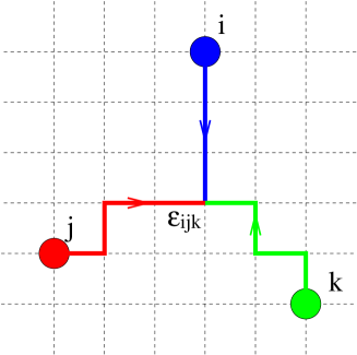
Figure 1: A possible configuration of flux lines in a baryon on the lattice.

The model is motivated from the strong coupling limit of HLGT, where there are “flux lines” which play the role of glue. In the adiabatic approximation operators which make the quarks move are neglected. The plaquette operator corrects the strong coupling limit, and induces motion of the “flux lines” between the quarks and the junction perpendicular to their rest positions. The flux lines are modeled by equally spaced “beads” of identical mass, so that the energy of each flux line is proportional to the number of beads, and hence its length. The spacing of the beads along the rest positions of the flux lines can be thought of as a finite lattice spacing, and the beads are allowed to move perpendicular to their rest position. The beads are attracted to each other by a linear potential, and the resulting discretized flux lines vibrate in various modes. Global color invariance requires that the three flux lines emanating from the quarks meet at a junction, which is also modeled by a bead. It is shown in HLGT that a single plaquette operator can move the junction and retain the Y-shaped string with the links in their ground state (see Fig. 2 and Appendix A), so that the junction may have a similar mass to the beads. However, for generality we allow the junction to have a different mass associated with it than that of the other beads.

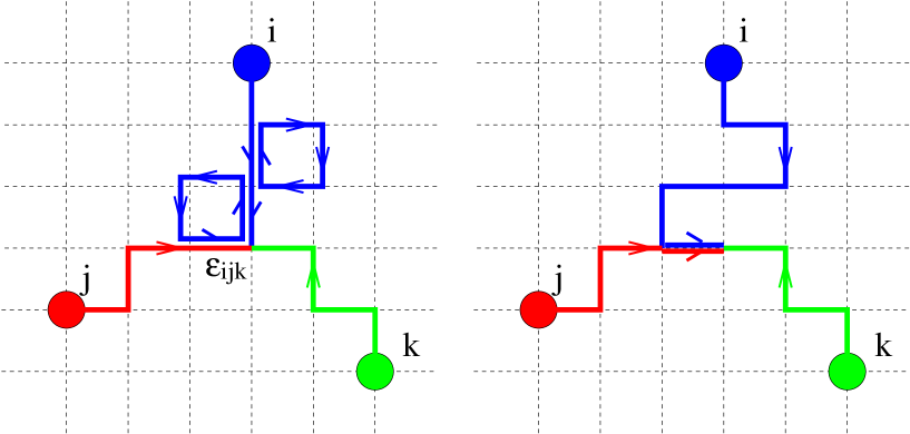
Figure 2: Flux lines in a baryon on the lattice, illustrating the application of a pair of plaquette operators, the upper operator moving one flux line perpendicular to its starting position, and the lower attempting to move the junction.

The final picture of both conventional and hybrid baryons is that of three quarks, connected via a line of beads to the junction in a Y-shaped configuration. The potential between neighboring beads is linear. The adiabatic approximation is used, so that the string is assumed to adjust its state quickly in response to motion of the quarks, thus generating a potential in which the quarks move, in both conventional and hybrid baryons. The motion of the quarks in these potentials is then solved for variationally. A brief outline of this approach is given in Ref. CP1 . The purpose of the present paper is to describe the model and the calculation of hybrid baryon masses in much more detail, and to put this work in the context of recent advances in lattice gauge theory.

Table 1: Notations frequently used in the main text.

$b$	string tension
$\theta_{J}$	angle between triads suspended at the equilibrium junction position
$i=1,2,3$	quark or triad label
$N_{i}$	number of beads on triad $i$
$n=1,N_{i}$	counts the beads on triad $i$ from quark $i$ to the junction
$m=1,N_{i}$	counts the modes of the triad $i$
$M_{i}$	mass of quark $i$
$m_{b}$	mass of the beads
$m_{J}$	mass of the junction
$l_{i}$	distance from the equilibrium junction position to quark $i$
$\hat{{\mbox{\boldmath$l$}}}_{i}$	direction from the equilibrium junction position to quark $i$
${\bf r}_{i}$	position of quark $i$
$q_{\parallel m}^{i}$	amplitude of mode $m$ on triad $i$ in the $QQQ$ plane, but perpendicular to $\hat{{\mbox{\boldmath$l$}}}_{i}$
$q_{\perp m}^{i}$	amplitude of mode $m$ on triad $i$ perpendicular to the $QQQ$ plane
${\bf r}=(x,y,z)$	cartesian coordinates of the junction
${\mbox{\boldmath$\hat{\eta}$}}_{\pm},\;{\mbox{\boldmath$\hat{\eta}$}}_{z}$	junction oscillation directions parallel and perpendicular to the $QQQ$ plane, respectively
$\omega_{\pm},\;\omega_{z}$	junction oscillation frequencies parallel and perpendicular to the $QQQ$ plane, respectively

The rest of the paper is organized as follows. Section II describes the dynamics of the flux tubes in various quark configurations, with analytic solutions in special cases. Section III discusses the quark-label exchange symmetry, parity, and chirality of the flux configuration. In Section IV, the orbital angular momentum and color of the flux, and the combined quark and flux wave function are constructed. The following Section V describes the potential in which the quarks move, which includes the energy of the flux. Numerical estimates of the masses of hybrid baryons are given in Section VI. In Sections VII and VIII further discussions and conclusions are given.

II Flux Dynamics

Denote by $\theta_{132}$ the angle between the line from quark 1 to 3 and that from quark 2 to 3. If $\theta_{123}$, $\theta_{132}$, and $\theta_{213}$ are all smaller than $120^{\rm o}$, the flux is in its equilibrium (lowest-energy) configuration when the junction is located such that there are angles of $120^{\rm o}$ between each of the triads that connect each of the quarks to the junction, and the beads all lie on the triads. In this lowest energy configuration, the string lies in the plane defined by the three quarks, denoted by the $QQQ$ plane. The angle between the line from any two quarks to the junction equilibrium position ${\bf r}_{\mbox{eq}}$ is $120^{\rm o}$, which is denoted by $\theta_{J}=120^{\rm o}$ (see Fig. 3 and Table 1).

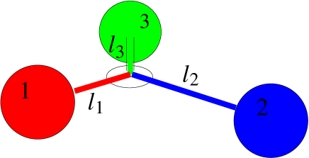
Figure 3: Flux configuration when none of the angles in the triangle joining the quarks are larger than 120^o.

In terms of the lengths $l_{i}$ of the lines from the $i$-th quark to the junction, and the quark positions ${\bf r}_{i}$, the equilibrium junction position is

$${\bf r}_{\mbox{eq}}=\frac{l_{2}l_{3}{\bf r}_{1}+l_{1}l_{3}{\bf r}_{2}+l_{1}l_{2}{\bf r}_{3}}{l_{2}l_{3}+l_{1}l_{3}+l_{1}l_{2}}.$$ (1)

The position vectors of the quarks relative to the junction equilibrium position are ${\mbox{\boldmath$l$}}_{i}={\bf r}_{i}-{\bf r}_{\mbox{eq}}$.

If one of $\theta_{123}$, $\theta_{132}$, and $\theta_{213}$ is larger than or equal to $120^{\rm o}$, the equilibrium configuration of the flux is not this Y-shaped configuration. If $\theta_{ijk}>120^{\rm o}$, the lowest energy configuration has the junction at the position of quark $j$ (see Fig. 4). This situation is denoted by $\theta_{J}>120^{o}$. In what follows the case where $\theta_{132}>120^{\rm o}$ is analyzed, but the formulae for the other cases follow by the appropriate label exchange.

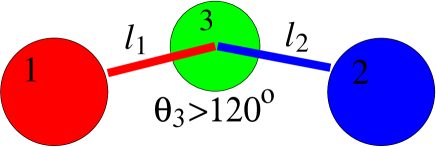
Figure 4: Flux configuration when one of the angles in the triangle joining the quarks, here $\theta_{132}$, is larger than 120^o.

An axis system is chosen as indicated in Figure 5.

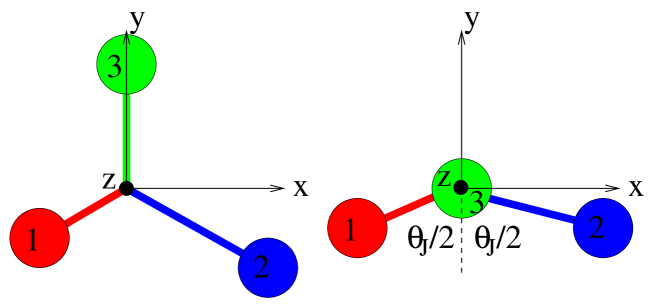
Figure 5: Coordinate system used to describe motion of the flux in the QQQ plane, for configurations with (a) all of $\theta_{123}$, $\theta_{132}$, and $\theta_{213}$ less than 120^o and (b) with $\theta_{J}=\theta_{132}$ larger than 120^o.

This defines normalized $\hat{\bf x}$ and $\hat{\bf y}$, which can also be written in the $\theta_{J}=120^{\rm o}$ case as

$$\hat{\bf x}=-\frac{\hat{{\mbox{\boldmath$l$}}}_{1}-\hat{{\mbox{\boldmath$l$}}}_{2}}{\sqrt{3}}\hskip 28.45274pt\hat{\bf y}=-\frac{\hat{{\mbox{\boldmath$l$}}}_{1}+\hat{{\mbox{\boldmath$l$}}}_{2}-2\hat{{\mbox{\boldmath$l$}}}_{3}}{3},$$ (2)

where the $\hat{{\mbox{\boldmath$l$}}}_{i}$ are unit vectors along the triads, and $\hat{{\mbox{\boldmath$l$}}}_{1}+\hat{{\mbox{\boldmath$l$}}}_{2}+\hat{{\mbox{\boldmath$l$}}}_{3}=0$, so that $\hat{\bf y}$ equals $\hat{{\mbox{\boldmath$l$}}}_{3}$ and $\hat{\bf x}$ is perpendicular to $\hat{{\mbox{\boldmath$l$}}}_{3}$. The third triad lies on the positive $y$-axis and the other two triads are $120^{\rm o}$ on either side of the $y$-axis: triad one on the left-hand and triad two on the right-hand side. It is assumed that the sum of the masses of the beads and the junction is the energy of the flux configuration in its equilibrium position, so that

$$m_{b}\sum_{i=1}^{3}N_{i}+m_{J}=b\sum_{i=1}^{3}l_{i},$$ (3)

which implies

$$m_{b}=\frac{b\sum_{i=1}^{3}l_{i}}{\sum_{i=1}^{3}N_{i}+\frac{m_{J}}{m_{b}}},$$ (4)

where $N_{i}$ is the number of beads on triad $i$. Note from the above that the bead mass $m_{b}$ is determined by the string tension $b$, the triad lengths $l_{i}$, and the ratio $m_{J}/m_{b}$, and so should not be regarded as an independent parameter.

II.1 Hamiltonian for $\theta_{J}=120^{o}$ case

The flux configuration is made dynamical by allowing the junction and the beads to vibrate with respect to their equilibrium configuration. There are two important motions which are expected to have physical significance: (1) the motion of the junction perpendicular to and within the plane relative to its rest position, denoted “junction motion”, and (2) the motion of the beads in the two directions perpendicular to the line connecting the quark to the junction, called “bead motion”, as illustrated in Fig. 6.

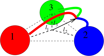
Figure 6: Motion of the flux configuration decomposed into “junction motion” and “bead motion”.

The bead motion coordinates are not their positions, but the oscillating-wave amplitudes (defined in Appendix B) of the beads relative to their rest positions on the triads. It is important for what follows that the bead position coordinates are defined relative to their rest positions on the triads between the quarks and junction, which have followed the junction motion (see Fig. 7).

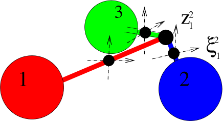
Figure 7: Coordinates used to describe the motion of the beads in the presence of a displaced junction.

The Hamiltonian is written in terms of the junction and bead motion coordinates. In what follows the small-oscillations approximation is used, where the beads and junction remain close to their positions in the equilibrium configuration. This approximation is used to motivate the basis of the subsequent numerical treatment, which is that it is a reasonable approximation to treat the flux motion as that of the junction, with an effective mass which depends on the equilibrium lengths of the triads, among other quantities. In the numerical treatment that follows, the restriction to small oscillations is removed.

As the string moves, the quarks are allowed to move with fixed positions relative to each other, in order to keep the center of mass fixed. This is called the “redefined adiabatic” approximation. By working in this approximation, some but not all non-adiabatic effects are incorporated.

The flux Hamiltonian for the $\theta_{J}=120^{\rm o}$ case in the redefined adiabatic approximation is (see Appendix B)

$$H_{\mbox{\small flux}} = \frac{1}{2}M_{\mbox{\small eff}}{\bf\dot{r}}^{2}+V_{\mbox{\small J}}^{\mbox{\small sm.osc.}}$$ (5)

$$+ \frac{1}{2}m_{\mbox{\small eff}}\sum_{i=1}^{3}\frac{N_{i}+1}{2}\sum_{m=1}^{N_{i}}\left[({{\dot{q}}_{\parallel m}^{i})}^{2}+{({\dot{q}}_{\perp m}^{i})}^{2}\right]+\frac{b}{2}\sum_{i=1}^{3}l_{i}\sum_{m=1}^{N_{i}}\frac{1}{2}(\omega^{i}_{m})^{2}\left[(q_{\parallel m}^{i})^{2}+(q_{\perp m}^{i})^{2}\right]$$

$$+ m_{b}\;{\bf\dot{r}}\cdot\sum_{i=1}^{3}\sum_{m=1}^{N_{i}}\left[\beta^{i}_{m}-\frac{m_{b}}{2}\;\frac{\sum_{k=1}^{3}N_{k}+2\frac{m_{J}}{m_{b}}}{\sum_{k=1}^{3}(bl_{k}+M_{k})}\;\alpha^{i}_{m}\right]\left(e^{i}_{x}{\dot{q}}_{\parallel m}^{i},e^{i}_{y}{\dot{q}}_{\parallel m}^{i},{\dot{q}}_{\perp m}^{i}\right)$$

$$- \frac{m_{b}^{2}}{2}\frac{1}{\sum_{i=1}^{3}(bl_{i}+M_{i})}\left\{\sum_{i=1}^{3}\sum_{n\neq m}^{N_{i}}\alpha^{i}_{n}\alpha^{i}_{m}({\dot{q}}_{\parallel n}^{i}{\dot{q}}_{\parallel m}^{i}+{\dot{q}}_{\perp n}^{i}{\dot{q}}_{\perp m}^{i})\right.$$

$$+\sum_{i\neq j}^{3}\sum_{n=1}^{N_{i}}\sum_{m=1}^{N_{j}}\alpha^{i}_{n}\alpha^{j}_{m}\left[\mbox{\boldmath$e$}^{i}\cdot\mbox{\boldmath$e$}^{j}{\dot{q}}_{\parallel n}^{i}{\dot{q}}_{\parallel m}^{j}+{\dot{q}}_{\perp n}^{i}{\dot{q}}_{\perp m}^{j}\right]$$

$$\left.+\sum_{i=1}^{3}\sum_{m=1}^{N_{i}}\left[(\alpha^{i}_{m})^{2}-\frac{N_{i}+1}{2}\right]\left[({\dot{q}}_{\parallel m}^{i})^{2}+({\dot{q}}_{\perp m}^{i})^{2}\right].\right\}$$

The first term in Eq. 5 is the kinetic energy of the junction, with an effective mass of

$$M_{\mbox{\small eff}}\equiv m_{b}\left[\sum_{i=1}^{3}\frac{N_{i}(2N_{i}+1)}{6(N_{i}+1)}+\frac{m_{J}}{m_{b}}-\frac{m_{b}{(\sum_{i=1}^{3}N_{i}+2\frac{m_{J}}{m_{b}})}^{2}}{4(\sum_{i=1}^{3}(bl_{i}+M_{i}))}\right],$$ (6)

where the last term in Eq. 6 arises from the center-of-mass correction, and the first from the trivial motion of the beads which accompanies motion of the junction. The second term in Eq. 5 is the potential energy of the junction in the small-oscillations approximation, given in terms of the coordinates ${\bf r}\equiv(x,y,z)$ defined in Fig. 5 by

$$V_{\mbox{\small J}}^{\mbox{\small sm.osc.}} \equiv b\sum_{i=1}^{3}l_{i}$$ (7)

$$+ \frac{b}{2}\left[x^{2}\left(\frac{1}{4l_{1}}+\frac{1}{4l_{2}}+\frac{1}{l_{3}}\right)+\frac{3}{4}y^{2}\left(\frac{1}{l_{1}}+\frac{1}{l_{2}}\right)-\frac{\sqrt{3}}{2}xy\left(\frac{1}{l_{1}}-\frac{1}{l_{2}}\right)+z^{2}\left(\frac{1}{l_{1}}+\frac{1}{l_{2}}+\frac{1}{l_{3}}\right)\right].$$

The third and fourth terms in Eq. 5 are the kinetic and potential energies of the beads, respectively, written in terms of the effective mass of the beads, including a center-of-mass correction,

$$m_{\mbox{\small eff}}\equiv m_{b}\left(1-\frac{m_{b}}{\sum_{i=1}^{3}(bl_{i}+M_{i})}\right),$$ (8)

and the frequency of the $m$-th normal mode on the $i$-th triad,

$$\omega^{i}_{m}\equiv\frac{2(N_{i}+1)}{l_{i}}\sin\frac{m\pi}{2(N_{i}+1)}.$$ (9)

The fifth and sixth terms in Eq. 5 represent interactions between the junction and the beads, and interactions among the beads, respectively. In these terms the vectors $\mbox{\boldmath$e$}^{i}$ are defined to be perpendicular to $\hat{{\mbox{\boldmath$l$}}}_{i}$, so that

$$\mbox{\boldmath$e$}^{1}=\left(-\frac{1}{2},\frac{\sqrt{3}}{2},0\right),\hskip 19.91684pt\mbox{\boldmath$e$}^{2}=\left(-\frac{1}{2},-\frac{\sqrt{3}}{2},0\right),\hskip 19.91684pt\mbox{\boldmath$e$}^{3}=\left(1,0,0\right),\hskip 19.91684pt\mbox{\boldmath$e$}^{i}\cdot\mbox{\boldmath$e$}^{j}=-\frac{1}{2}.$$ (10)

In terms of the amplitudes $\mbox{\boldmath$q$}_{m}^{i}$ of the $m$-th normal mode on the $i$-th triad, where displacements of the beads along the triads are not allowed, the coordinates $q_{\parallel m}^{i}=\mbox{\boldmath$e$}^{i}\cdot\mbox{\boldmath$q$}_{m}^{i}$ are the projections in the QQQ plane, and the coordinates $q_{\perp m}^{i}$ are the projections of these amplitudes out of the QQQ plane. Finally, the $\beta^{i}_{m}$ and $\alpha^{i}_{m}$ are the sums

$$\beta^{i}_{m}\equiv\sum_{p=1}^{N_{i}}\frac{p}{N_{i}+1}\sin\frac{mp\pi}{N_{i}+1}=\frac{(-1)^{m+1}}{2}\cot\frac{m\pi}{2(N_{i}+1)}$$ (11)

and

$$\alpha^{i}_{m}\equiv\sum_{p=1}^{N_{i}}\sin\frac{mp\pi}{N_{i}+1}=\begin{cases}0&m={\rm even}\\ \cot\frac{m\pi}{2(N_{i}+1)}&m={\rm odd}.\end{cases}$$ (12)

The above demonstrates that the Hamiltonian can be seperated into three parts. The first (the first two terms in Eq. 5) corresponds to the motion of the junction in the absence of beads, with an effective junction mass related to its own mass and the bead mass, with a center-of-mass correction for finite quark masses. The second part (terms three and four) is the independent motion of the beads on the three triads with respect to a fixed junction, with a bead mass also corrected for center-of-mass motion for finite quark masses. There is also an “interaction” part where the junction interacts with the various bead modes (term five), where the bead modes associated with the same quark interact with each other, and where the modes on triads corresponding to different quarks interact with each other (term six). Note that these bead self-interactions (term six) vanish for infinite quark masses.

Because the quarks move with fixed relative positions only to maintain the center of mass position in the presence of a moving junction and beads, there are no quark kinetic terms in this string Hamiltonian, and there is no sense in which the quarks acquire mass from the beads, i.e. constituent quark masses are not derived from current quark masses.

Note that the model predicts that for bead motion in the small-oscillations approximation the potential has the customary, and phenomenologically important capstick86 , linear potential term $b\sum_{i=1}^{3}l_{i}$ (see Eq. 7). For large $l_{i}$, where the small-oscillations approximation becomes exact, the potential is just the linear term expected in any string model. This potential is a prediction of the model, not an ansatz. In the numerical work that follows, the small-oscillations approximation for the junction will be removed to yield the potential energy in the absence of beads, i.e.

$$V_{\mbox{\small J}}\equiv b\left(\sqrt{\left(\frac{\sqrt{3}}{2}l_{1}+x\right)^{2}+\left(\frac{l_{1}}{2}+y\right)^{2}+z^{2}}\right.$$ (13)

$$\left.+\sqrt{\left(\frac{\sqrt{3}}{2}l_{2}-x\right)^{2}+\left(\frac{l_{2}}{2}+y\right)^{2}+z^{2}}+\sqrt{x^{2}+(l_{3}-y)^{2}+z^{2}}\right).$$

II.2 Hamiltonian for $\theta_{J}>120^{o}$ case

The correct expression in the small-oscillations approximation for the flux Hamiltonian for the case $\theta_{J}>120^{o}$ can be obtained (see Appendix B) by setting $l_{3}=N_{3}=0$ in $H_{\mbox{\small flux}}$, $M_{\mbox{\small eff}}$, and $m_{\mbox{\small eff}}$ in Eqs. 5, 6, and 8, and $q_{\parallel m}^{3}$, $q_{\perp m}^{3}=0$ in $H_{\mbox{\small flux}}$ in Eq. 5, and changing the junction potential energy in Eq. 7 to

$$V_{\mbox{\small J}}^{\mbox{\small sm.osc.}}\equiv b\sum_{i=1}^{2}l_{i}\;+2by\cos\frac{\theta_{J}}{2}+b\sqrt{x^{2}+y^{2}+z^{2}}$$ (14)

$$+\;\frac{b}{2}\left(\left[x^{2}\cos^{2}\frac{\theta_{J}}{2}+y^{2}\sin^{2}\frac{\theta_{J}}{2}+z^{2}\right]\left\{\frac{1}{l_{1}}+\frac{1}{l_{2}}\right\}-2xy\sin\frac{\theta_{J}}{2}\cos\frac{\theta_{J}}{2}\left\{\frac{1}{l_{1}}-\frac{1}{l_{2}}\right\}\right).$$

Note that the third term above, which is the length of the third triad when the junction has moved, cannot be expanded in the small-oscillations approximation. The vectors $\mbox{\boldmath$e$}^{i}$ become

$$\mbox{\boldmath$e$}^{1}=\left(-\cos\frac{\theta_{J}}{2},\sin\frac{\theta_{J}}{2},0\right),\hskip 19.91684pt\mbox{\boldmath$e$}^{2}=\left(-\cos\frac{\theta_{J}}{2},-\sin\frac{\theta_{J}}{2},0\right).$$ (15)

In the numerical work that follows, the small-oscillations approximation for the junction will be removed to yield the potential energy in the absence of beads,

$$V_{\mbox{\small J}}\equiv b\left(\sqrt{(l_{1}\sin\frac{\theta_{J}}{2}+x)^{2}+(l_{1}\cos\frac{\theta_{J}}{2}+y)^{2}+z^{2}}\right.$$ (16)

$$\left.+\sqrt{(l_{2}\sin\frac{\theta_{J}}{2}-x)^{2}+(l_{2}\cos\frac{\theta_{J}}{2}+y)^{2}+z^{2}}+\sqrt{x^{2}+y^{2}+z^{2}}\right).$$

II.3 Approximate flux Hamiltonian

It will now be demonstrated that the interaction terms in Eq. 5 (terms five and six) give a minor contribution in the small-oscillations approximation. The free parameters in the model (and the values initially used for the numerical simulation) are the string tension ($0.18$ GeV²), the ratio of the junction and bead masses (1), and the quark masses ($0.33$ GeV). The simulation is performed with one bead between each quark and the junction, and the quarks at first form an equilateral triangle with the lengths of the triads given a typical value of $2.5$ GeV^-1.

For the purposes of this demonstration, the problem is first solved numerically without approximations, by solving the classical Euler-Lagrange equations of motion rather than using quantum mechanics. This solution should provide a good indicator of how the mode frequences with and without the interaction Hamiltonian compare. The mode frequencies parallel and perpendicular to the plane are (in GeV)

Parallel	0.607	0.607	0.924	1.08	1.08
Perpendicular	0.828		0.924	0.924	1.37

where the lowest frequencies have been identified in bold face. If the interaction Hamiltonian is set to zero, the number of modes does not change, as the number of degrees of freedom (three junction coordinates and two transverse bead coordinates per bead) is unchanged. Since the junction and bead degrees of freedom become uncoupled, it is possible to identify modes involving junction motion and those involving bead motion. The mode frequencies (in GeV) corresponding to the junction motion (bold) and bead vibrations are

Parallel	0.614	0.614	1.00	1.00	1.00
Perpendicular	0.869		1.00	1.00	1.00

The similarity of the frequencies of the lowest energy modes in this approximation to those arising from the full Hamiltonian (a deviation of 1% in the case of the modes with motion parallel to the QQQ plane, and 5% for the mode perpendicular to the plane) shows that for these lowest energy modes the interaction Hamiltonian can be safely neglected. In retrospect, the reason for this is because of the choice of physically appropriate coordinates for the problem, i.e. the junction coordinates and the coordinates of the beads transverse to the triads joining the junction to the quarks (see Fig. 7).

To ensure that this result is not dependent on this choice of QQQ configuration or the parameters in the Hamiltonian, the parameters were varied independently around the central values used above. Quark masses up to the charm quark mass of $1.5$ GeV were used, the ratio of the junction to the bead mass was taken up to 10, and the triads were given lengths from $0.5-5$ GeV^-1, and cases with unequal lengths were tested. The percentage difference between all nine mode frequencies calculated with the full Hamiltonian and with the interaction terms neglected is shown for selected parameters in Table 2. The largest error for the two lightest parallel modes and the lightest perpendicular mode, shown in bold face, is 7%. This demonstrates that, to a good approximation, the dynamics of the three lowest frequency modes can be simplified to junction and bead motion which are independent of one another. The bead motion on various triads, and bead motion in various modes on the same triad are to a good approximation independent of each other.

Table 2: Percentage differences between all nine mode frequencies obtained in the one bead per triad problem for the full Hamiltonian (Eq. 5) and the Hamiltonian with the interaction terms (the last two terms in Eq. 5) neglected, for selected parameters. The first group of five percentage differences is for parallel mode frequencies, the last four for perpendicular mode frequencies. Within each group the percentage differences are displayed from left to right for in ascending order of mode frequency. Quark masses are in GeV and triad lengths in GeV^-1.

$M_{1}$	$M_{2}$	$M_{3}$	$\frac{m_{J}}{m_{b}}$	$l_{1}$	$l_{2}$	$l_{3}$	Percentage difference (%)
0.33	0.33	0.33	1	2.5	2.5	2.5	1	1	8	8	8	5	8	8	37
1.5	0.33	0.33	1	2.5	2.5	2.5	2	2	5	11	11	7	5	5	40
0.33	0.33	0.33	10	2.5	2.5	2.5	0	0	2	1	1	0	2	2	5
0.33	0.33	0.33	1	0.5	2.5	2.5	1	6	9	2	4	7	0	10	11
0.33	0.33	0.33	1	5	2.5	2.5	1	1	0	2	7	3	2	8	28
0.33	0.33	0.33	1	0.5	2.5	5	1	1	2	1	3	2	0	4	10

The frequencies can be followed from the non-interacting case as interactions are turned on, and level crossing does not occur. Hence mode frequencies for the fully-interacting Hamiltonian can be uniquely associated with modes frequencies obtained with interactions neglected. The lowest frequency is always associated with the lowest junction excitation. However, the next lowest frequency can be associated with the second junction excitation or with a bead excitation along a triad when the QQQ configuration is asymmetric. This work focuses on the lowest lying excitation of the flux configuration, always corresponding to junction motion, but it should be kept in mind that the next lowest hybrid baryon may involve bead excitation.

The equal-mass three-bead model is unrealistic when one of the triads is short, since the mass of the bead on the short triad is not representative of the energy stored in the triad on which it lies. An alternative model has been considered where the bead mass is taken to be proportional to the length of the triad, but the sum of the bead masses and junction mass still equals the energy stored in the Y-shaped string configuration (Eq. 3 with $N_{i}=1$). In this model it is found that the low-lying frequencies for the full Hamiltonian are very similar to the former model, with similar small errors induced by neglecting the interaction terms in the Hamiltonian of Eq. 5.

II.4 Analytical solution of the flux Hamiltonian

For the Hamiltonian in Eq. 5 (the $\theta_{J}=120^{o}$ case) the last two terms have been shown to be negligible for the lowest frequency in the small-oscillations approximation, in the case where there is one bead on each triad, and these terms are neglected in what follows. What follows is, therefore, based on the approximate $\theta_{J}=120^{o}$ Hamiltonian

$${\tilde{H}}_{\mbox{\small flux}} \equiv \frac{1}{2}M_{\mbox{\small eff}}{\bf\dot{r}}^{2}+V_{\mbox{\small J}}+\frac{1}{2}m_{\mbox{\small eff}}\sum_{i=1}^{3}\frac{N_{i}+1}{2}\sum_{m=1}^{N_{i}}\left[(\dot{q}_{\parallel m}^{i})^{2}+(\dot{q}_{\perp m}^{i})^{2}\right]$$ (17)

$$+\frac{b}{2}\sum_{i=1}^{3}l_{i}\sum_{m=1}^{N_{i}}\frac{1}{2}(\omega^{i}_{m})^{2}\left[(q_{\parallel m}^{i})^{2}+(q_{\perp m}^{i})^{2}\right],$$

with $V_{\mbox{\small J}}$ given by Eq. 13. Note that since the $q_{\parallel m}^{i}$, $q_{\perp m}^{i}$ are defined with respect to the line from the junction to the quarks, they depend implicitly on ${\bf r}$. The corresponding Hamiltonian for $\theta_{J}>120^{o}$ is obtained by setting $l_{3}=N_{3}=0$ in $M_{\mbox{\small eff}}$ and $m_{\mbox{\small eff}}$ in Eqs. 6 and 8, and restricting the summation in Eq. 17 to $i=1,2$, with $V_{\mbox{\small J}}$ given by Eq. 16.

Since Eq. 17 is diagonal in the coordinates of the beads, the last two terms in Eq. 17, corresponding to the bead energies, can be replaced by their ground-state harmonic oscillator energies

$${\tilde{H}}_{\mbox{\small flux}}=\frac{1}{2}M_{\mbox{\small eff}}{\bf\dot{r}^{2}}+V_{\mbox{\small J}}+\sum_{i=1}^{3}\sqrt{\frac{bl_{i}}{m_{\mbox{\small eff}}(N_{i}+1)}}\sum_{m=1}^{N_{i}}\omega^{i}_{m},$$ (18)

which is summed over the two polarizations possible for each bead vibration. The sum of the frequencies is

$$\sum_{m=1}^{N_{i}}\omega^{i}_{m}=\sqrt{2}\frac{N_{i}+1}{l_{i}}\frac{\sin\frac{N_{i}\pi}{4(N_{i}+1)}}{\sin\frac{\pi}{4(N_{i}+1)}}.$$ (19)

If the number of beads is taken to infinity, the dependence of the Hamiltonian on the (unphysical) number of beads can be removed. The part of the Hamiltonian in Eq. 18 arising from the beads becomes infinite when $N_{i}\rightarrow\infty$. To avoid infinite energies, the bead separation regularization parameter (analogous to the lattice spacing) $a\equiv l_{i}/(N_{i}+1)$ is fixed when $N_{i}\rightarrow\infty$. This is consistent with the flux-tube model philosophy that $a$ cannot be chosen arbitrarily small, since that would lead to the breakdown of the strong coupling expansion of the Hamiltonian formulation of QCD, from which the model is motivated paton85 . Taking $N_{i}\rightarrow\infty$, while keeping $a$ fixed, the Hamiltonian becomes paton85

$${\tilde{H}}_{\mbox{\small flux}}^{\infty}=\frac{1}{2}M_{\mbox{\small eff}}^{\infty}{\bf\dot{r}^{2}}+V_{\mbox{\small J}}+\sum_{i=1}^{3}\left[\frac{4l_{i}}{\pi a^{2}}-\frac{1}{a}-\frac{\pi}{12l_{i}}+{\cal O}(a^{2})+\cdots\right],$$ (20)

with

$$M_{\mbox{\small eff}}^{\infty}\equiv b\sum_{i=1}^{3}l_{i}\left(\frac{1}{3}-\frac{b\sum_{i=1}^{3}l_{i}}{4\sum_{i=1}^{3}(bl_{i}+M_{i})}\right),$$ (21)

where ${\tilde{H}}_{\mbox{\small flux}}^{\infty}$ is now independent of the (unknown) ratio $m_{J}/m_{b}$. Since $N_{i}\rightarrow\infty$ with $a$ fixed, the part of the Hamiltonian in Eq. 20 arising from the beads is valid only in the limit $l_{i}\rightarrow\infty$.

The part of the Hamiltonian in Eq. 20 arising from the beads contains a linear term $4l_{i}/\pi a^{2}$ and a constant term $-1/a$, which are regularization-scheme dependent terms in the “self energy” of the string system. As explained in Ref. paton85 , the linear term should be regarded as a contribution that renormalizes the bare string tension $b$ to its physical value. The constant term is three times larger than the constant term found for mesons paton85 . The Luscher luscher term $-\pi/12l_{i}$ is regularization-scheme independent and finite, and can be regarded as a prediction of the flux-tube model, although it is insignificant at large $l_{i}$, where its derivation is valid. The Luscher term arises in relativistic string theories luscher in the limit $l_{i}\rightarrow\infty$. In this limit the string excitations in our model coincide with relativistic string theories. There exists strong lattice-QCD evidence, through the study of “torelons”, of the existence of the Luscher term in QCD stephenson . The form of the Luscher term should be contrasted with that of a Coulomb term, with the former depending inversely on the triad lengths, and the latter inversely on the distance between two quarks.

The Hamiltonian for the $\theta_{J}>120^{o}$ case is obtained by setting $l_{3}=0$ in $M_{\mbox{\small eff}}^{\infty}$ in Eq. 21, and restricting the summation in Eq. 20 to $i=1,2$ with $V_{\mbox{\small J}}$ from Eq. 16.

If the redefined adiabatic approximation was not made, i.e. if the calculation was not performed in the center of mass frame of the entire system with the distances between the quarks fixed, then $M_{\mbox{\small eff}}^{\infty}=b\sum l_{i}/3$. The correction from center-of-mass motion in Eq. 21 substantially reduces the effective mass of the junction. It is shown below that the excitation energies of the junction are proportional to $(M_{\mbox{\small eff}}^{\infty})^{-\frac{1}{2}}$ (see Eqs. 30–31), and so with typical QQQ configurations the junction excitation energies are 1 to 2 times larger in the redefined adiabatic approximation than in the adiabatic approximation. This underlines the importance of working in the CM frame.

The ground state bead configuration that solves the Hamiltonian of Eq. 17 is

$$\Phi = \lim_{N_{i}\rightarrow\infty}\prod^{3}_{i=1}\pi^{-\frac{N_{i}}{2}}\prod_{m=1}^{N_{i}}(m_{\mbox{\small eff}}bl_{i}(N_{i}+1))^{\frac{1}{4}}\sqrt{\frac{\omega^{i}_{m}}{2}}$$ (22)

$$\exp\left\{-\frac{1}{2}\sum_{i=1}^{3}\sum_{m=1}^{N_{i}}\sqrt{m_{\mbox{\small eff}}bl_{i}(N_{i}+1)}\,\frac{\omega^{i}_{m}}{2}\left[(q_{\parallel m}^{i})^{2}+(q_{\perp m}^{i})^{2}\right]\right\},$$

in the limit $N_{i}\rightarrow\infty$ (with $a$ fixed) that is used to express the Hamiltonian in Eq. 20. The corresponding wave function for $\theta_{J}>120^{o}$ is obtained by restricting the products in Eq. 22 to $i=1,2$, and setting $l_{3}=0$ in $m_{\mbox{\small eff}}$ in Eq. 8.

II.5 Analytic small-oscillations solution to the junction Hamiltonian for $\theta_{J}=120^{o}$

Define

$${{\mbox{\boldmath$\rho$}}}\equiv\frac{{\bf r}_{1}-{\bf r}_{2}}{\sqrt{2}}\hskip 28.45274pt{{\mbox{\boldmath$\lambda$}}}\equiv\frac{{\bf r}_{1}+{\bf r}_{2}-2{\bf r}_{3}}{\sqrt{6}}\hskip 28.45274pt\cos\theta_{\rho\lambda}\equiv\frac{{\mbox{\boldmath$\rho$}}\cdot{\mbox{\boldmath$\lambda$}}}{\rho\lambda}.$$ (23)

The six Jacobi variables $\rho$, $\lambda$ consist of (1) four variables which specify the positions of the quarks in the $QQQ$ plane, $\rho\equiv|{\mbox{\boldmath$\rho$}}|$, $\lambda\equiv|{\mbox{\boldmath$\lambda$}}|$, and $\theta_{\rho\lambda}$ (the angle between $\rho$ and $\lambda$) and ${\phi_{\rho}}$ (the angle between $\rho$ and the space-fixed $x$-direction), and (2) two polar angles $\theta$, and $\phi$ which specify the orientation of the vector ${\mbox{\boldmath$\rho$}}\times{\mbox{\boldmath$\lambda$}}$ which lies perpendicular to the plane. The variables $\rho,\lambda$ and $\theta_{\rho\lambda}$ are rotational scalars. They are related to the triad lengths $l_{1}$, $l_{2}$, and $l_{3}$ by the relations

$$l_{1}={\cal N}\;(\rho^{2}+\rho\lambda\sin\theta_{\rho\lambda}+\sqrt{3}\rho\lambda\cos\theta_{\rho\lambda}) l_{2}={\cal N}\;(\rho^{2}+\rho\lambda\sin\theta_{\rho\lambda}-\sqrt{3}\rho\lambda\cos\theta_{\rho\lambda})$$

$$l_{3}={\cal N}\;(-\frac{\rho^{2}}{2}+\frac{3}{2}\lambda^{2}+\rho\lambda\sin\theta_{\rho\lambda}) {\cal N}^{-1}=\sqrt{\frac{3}{2}(\rho^{2}+\lambda^{2})+3\rho\lambda\sin\theta_{\rho\lambda}}.$$ (24)

In the remainder of this section junction motion is treated in the small-oscillations approximation for the $\theta_{J}=120^{o}$ case. The junction Hamiltonian is $\frac{1}{2}M_{\mbox{\small eff}}^{\infty}{\bf\dot{r}^{2}}+V_{\mbox{\small J}}^{\mbox{\small sm.osc.}}$, where the potential is from Eq. 7. Junction motion in $(x,y)$ and out ($z$) of the QQQ plane are not coupled in $V_{\mbox{\small J}}^{\mbox{\small sm.osc.}}$, so motion along the $z$ direction is one of the vibrational modes of the junction. One way to define the $z$ direction in terms of the positions of the quarks is by the normalized vector

$${\mbox{\boldmath$\hat{\eta}$}}_{z}=\sigma_{z}\frac{{{\mbox{\boldmath$\rho$}}}\times{{\mbox{\boldmath$\lambda$}}}}{|{{\mbox{\boldmath$\rho$}}}\times{{\mbox{\boldmath$\lambda$}}}|},$$ (25)

where $\sigma_{z}$ denotes a sign that will be specified later. Note that $z$ motion of the junction motion occurs along the direction of the vector ${{\mbox{\boldmath$\rho$}}}\times{{\mbox{\boldmath$\lambda$}}}$, but there is no physical reason to prefer one sign $\sigma_{z}$ over the other.

The in-plane part of the Hamiltonian can be diagonalized in terms of the normalized eigenvectors 

$${\mbox{\boldmath$\hat{\eta}$}}_{\pm}=\frac{\sigma_{\pm}}{N(l_{1},l_{2},l_{3})}\left\{\left[\frac{1}{l_{3}}-\frac{1}{2}(\frac{1}{l_{1}}+\frac{1}{l_{2}})\pm\sqrt{s(l_{1},l_{2},l_{3})}\right]\hat{\bf x}+\frac{\sqrt{3}}{2}\{\frac{1}{l_{2}}-\frac{1}{l_{1}}\}\hat{\bf y}\right\},$$ (26)

where

$$s(l_{1},l_{2},l_{3})\equiv\frac{1}{l_{1}^{2}}+\frac{1}{l_{2}^{2}}+\frac{1}{l_{3}^{2}}-\frac{1}{l_{1}l_{2}}-\frac{1}{l_{1}l_{3}}-\frac{1}{l_{2}l_{3}}>0,$$ (27)

and

$$N(l_{1},l_{2},l_{3})\equiv\sqrt{2}\sqrt{s(l_{1},l_{2},l_{3})\pm(\frac{1}{l_{3}}-\frac{1}{2}(\frac{1}{l_{1}}+\frac{1}{l_{2}}))\sqrt{s(l_{1},l_{2},l_{3})}},$$ (28)

and a sign $\sigma_{\pm}$ is included for the same reasons as above. The vectors ${\mbox{\boldmath$\hat{\eta}$}}_{z}$, ${\mbox{\boldmath$\hat{\eta}$}}_{+}$, and ${\mbox{\boldmath$\hat{\eta}$}}_{-}$ can be verified to be orthonormal vectors. The junction Hamiltonian can now be written as

$$\frac{1}{2}M_{\mbox{\small eff}}^{\infty}{\bf\dot{r}^{2}}+V_{\mbox{\small J}}^{\mbox{\small sm.osc.}}=b\sum_{i=1}^{3}l_{i}+$$ (29)

$$\frac{1}{2}M_{\mbox{\small eff}}^{\infty}\left[({\mbox{\boldmath$\hat{\eta}$}}_{+}\cdot{\bf\dot{r}})^{2}+({\mbox{\boldmath$\hat{\eta}$}}_{-}\cdot{\bf\dot{r}})^{2}+({\mbox{\boldmath$\hat{\eta}$}}_{z}\cdot{\bf\dot{r}})^{2}+\omega^{2}_{+}({\mbox{\boldmath$\hat{\eta}$}}_{+}\cdot{\bf r})^{2}+\omega^{2}_{-}({\mbox{\boldmath$\hat{\eta}$}}_{-}\cdot{\bf r})^{2}+\omega^{2}_{z}({\mbox{\boldmath$\hat{\eta}$}}_{z}\cdot{\bf r})^{2}\right],$$

where the vibrational frequencies are given by

$$\omega^{2}_{z}=\frac{b}{M_{\mbox{\small eff}}^{\infty}}(\frac{1}{l_{1}}+\frac{1}{l_{2}}+\frac{1}{l_{3}})$$ (30)

and

$$\omega^{2}_{\pm}=\frac{b}{2M_{\mbox{\small eff}}^{\infty}}\left(\frac{1}{l_{1}}+\frac{1}{l_{2}}+\frac{1}{l_{3}}\pm\sqrt{s(l_{1},l_{2},l_{3})}\right).$$ (31)

Note that the out-of-plane mode is always more energetic than the in-plane modes, since $\omega_{z}>\omega_{\pm}$, and that the in-plane modes have $\omega_{-}\leq\omega_{+}$, with degeneracy only when $l_{1}=l_{2}=l_{3}$.

Solving the Schrödinger equation corresponding to Eqs. 20 and 29 yields the ground-state energy, corresponding to the adiabatic potential for the quark motion in a conventional baryon, of

$$V_{B}(l_{1},l_{2},l_{3})=b\sum_{i=1}^{3}l_{i}+\frac{1}{2}(\omega_{+}+\omega_{-}+\omega_{z})+\sum_{i=1}^{3}\left[\frac{4l_{i}}{\pi a^{2}}-\frac{1}{a}-\frac{\pi}{12l_{i}}+{\cal O}(a^{2})+\cdots\right].$$ (32)

Junction excitations in the ${\mbox{\boldmath$\hat{\eta}$}}_{-}$, ${\mbox{\boldmath$\hat{\eta}$}}_{+}$, or ${\mbox{\boldmath$\hat{\eta}$}}_{z}$ directions yield adiabatic potentials for the quark motion in different low-lying hybrid baryons, denoted $H_{1}$, $H_{2}$, and $H_{3}$, ordered from least to most energetic. The hybrid baryon string energy (adiabatic potential) is that of the baryon in Eq. 32 with the term $\omega_{-}$, $\omega_{+}$ or $\omega_{z}$ added for $H_{1}$, $H_{2}$ or $H_{3}$ hybrid baryons, respectively. Note that these results neglect the junction-bead and bead-bead interactions, which has been demonstrated to be a good approximation only for the lowest energy ($\omega_{-}$) mode.

It is intriguing to note that the baryon potential in Eq. 32 serves as an analytical form to which the infinitely-heavy quark potentials calculated in lattice QCD can be fitted as a function of $l_{i}$. Furthermore, the $l_{i}$ dependence of the various hybrid baryon potentials are predicted. Potentials were also predicted in Ref. kalash . Comparisons to lattice results would be instructive at large $l_{i}$, for which Eq. 32 was derived. The physical string tension is $b-4/(\pi a^{2})$. The constant $-1/a$ term is regularization-scheme dependent, and hence not physical. Indeed, lattice calculations bali find the constant term regularization dependent, and proportional to $1/a$. The remaining terms do not depend on either $b$ or $a$ when $M_{i}\rightarrow\infty$, which is the limit in which lattice QCD potentials are evaluated, noting that $b/M_{\mbox{\small eff}}^{\infty}$ is independent of $b$ in this limit.

The normalized flux wave function of the baryon is

$$\Psi_{B}({\bf r})=\frac{(M_{\mbox{\small eff}}^{\infty})^{\frac{3}{4}}(\omega_{+}\omega_{-}\omega_{z})^{\frac{1}{4}}}{\pi^{\frac{3}{4}}}\exp\left\{-\frac{M_{\mbox{\small eff}}^{\infty}}{2}(\omega_{+}({\mbox{\boldmath$\hat{\eta}$}}_{+}\cdot{\bf r})^{2}+\omega_{-}({\mbox{\boldmath$\hat{\eta}$}}_{-}\cdot{\bf r})^{2}+\omega_{z}({\mbox{\boldmath$\hat{\eta}$}}_{z}\cdot{\bf r})^{2})\right\}\;\Phi,$$ (33)

where the bead wave function $\Phi$ in Eq. 22 has been incorporated. For the $H_{1}$, $H_{2}$, and $H_{3}$ hybrid baryons, respectively, the normalized flux wave functions are $\Psi_{H_{i}}({\bf r})$

$$\sqrt{2M_{\mbox{\small eff}}^{\infty}\omega_{-}}\;{\mbox{\boldmath$\hat{\eta}$}}_{-}\cdot{\bf r}\;\Psi_{B}({\bf r}),\hskip 28.45274pt\sqrt{2M_{\mbox{\small eff}}^{\infty}\omega_{+}}\;{\mbox{\boldmath$\hat{\eta}$}}_{+}\cdot{\bf r}\;\Psi_{B}({\bf r}),\hskip 28.45274pt\sqrt{2M_{\mbox{\small eff}}^{\infty}\omega_{z}}\;{\mbox{\boldmath$\hat{\eta}$}}_{z}\cdot{\bf r}\;\Psi_{B}({\bf r}).$$ (34)

II.6 Junction motion away from the small-oscillations limit

Eq. 16 cannot be expanded in the small-oscillations approximation to the junction motion. Without this approximation, i.e. where $V_{\mbox{\small J}}$ in ${\tilde{H}}_{\mbox{\small flux}}^{\infty}$ in Eq. 20 is taken from Eqs. 13 and 16 for the cases $\theta_{J}=120^{o}$ and $\theta_{J}>120^{o}$ respectively, the eigenfrequencies and eigenvectors cannot be solved for analytically.

The variational principle is used to separately minimize the expectation value of the Hamiltonian ${\tilde{H}}_{\mbox{\small flux}}^{\infty}$ by solving the Schrödinger equation for the conventional baryons and hybrids $H_{i}$ using the ansatz simple-harmonic-oscillator wave functions in Eqs. 33 and 34. The calculated energies are upper bounds for the true energies, according to the Hyleraas-Undheim theorem. The parameters of the ansatz wave functions no longer have the values that they had in the small-oscillations approximation, but need to be fitted. For example, the directions ${\mbox{\boldmath$\hat{\eta}$}}_{z}$, ${\mbox{\boldmath$\hat{\eta}$}}_{-}$, and ${\mbox{\boldmath$\hat{\eta}$}}_{+}$ are no longer given by Eqs. 25 and 26, but will be fixed by the variational principle.

Note that ${\tilde{H}}_{\mbox{\small flux}}^{\infty}$ (Eq. 20) is even under the discrete transformation $z\rightarrow-z$ since $V_{\mbox{\small J}}$ in Eqs. 13 and 16 only depends on $z^{2}$. This implies that the wave functions should be either odd or even under $z\rightarrow-z$. But since the wave functions are assumed to be of the form in Eqs. 33 and 34, it is not difficult to show that this implies that one of the junction vibrational modes, corresponding to ${\mbox{\boldmath$\hat{\eta}$}}_{z}$, is always perpendicular to the $QQQ$ plane. Note that ${\mbox{\boldmath$\hat{\eta}$}}_{-}$, ${\mbox{\boldmath$\hat{\eta}$}}_{+}$, and ${\mbox{\boldmath$\hat{\eta}$}}_{z}$ are required to be orthonormal in order to obtain orthonormal hybrid baryon wave functions in Eq. 34. This gives four variational parameters that specify the ansatz wave functions: $M_{\mbox{\small eff}}^{\infty}\omega_{-}$, $M_{\mbox{\small eff}}^{\infty}\omega_{+}$, $M_{\mbox{\small eff}}^{\infty}\omega_{z}$, and an angle that describes the ray in which ${\mbox{\boldmath$\hat{\eta}$}}_{-}$ lies in the plane relative to the $x$-direction defined in Fig. 5. The minimization is carried out with respect to these four variables.

III Flux Symmetry

III.1 Quark label exchange symmetry

Denote by $P_{12}$, $P_{13}$, and $P_{23}$ the permutations which exchange the labels of the quarks. Except for color, quark-spin and flavor labels, which will only be of interest later, exchange symmetry affects only position labels. Under such quark label permutations the positions of the quarks are exchanged, e.g. $P_{12}$ exchanges ${\bf r}_{1}\leftrightarrow{\bf r}_{2}$, but note that variables that are not functions of the ${\bf r}_{i}$ are unaffected. Since the physics does not depend on the quark position labelling convention, the flux Hamiltonian given by Eq. 5 should be exchange symmetric. As the equilibrium junction position ${\bf r}_{\mbox{eq}}$ in Eq. 1 is invariant under the $P_{ij}$, and ${\mbox{\boldmath$l$}}_{i}={\bf r}_{i}-{\bf r}_{\mbox{eq}}$, it follows that ${\mbox{\boldmath$l$}}_{i}\leftrightarrow{\mbox{\boldmath$l$}}_{j}$ under $P_{ij}$. Also, since the number of beads on the $i$-th triad is $N_{i}=l_{i}/a-1$, then $N_{i}\leftrightarrow N_{j}$ under $P_{ij}$. The potential $V_{\mbox{\small J}}$ in Eq. 13 can be written in the manifestly exchange-symmetric form

$$V_{\mbox{\small J}}=b\sum_{i=1}^{3}|{\bf r}_{i}-{\bf r}|,$$ (35)

noting that the junction position ${\bf r}$ is not determined by the positions of the quarks. This establishes that all quantities in the flux Hamiltonian in Eq. 5 for the $\theta_{J}=120^{o}$ case are invariant under exchange symmetry transformations.

Since the flux Hamiltonian is invariant under exchange symmetry, it is clear that energies (or adiabatic potentials) that are solutions of the flux Schrödinger equation are also exchange symmetric. This is explicit for the frequencies in Eqs. 30 and 31, and the potential in Eq. 32.

By the same arguments as above it can be shown that in the $\theta_{J}>120^{o}$ case, the Hamiltonian (Eq. 14) is invariant under $P_{12}$.

Since the Hamiltonian is exchange symmetric, the commutation relations $[H_{\mbox{\small flux}},P_{ij}]=0$ hold. This implies that the wave functions of conventional and hybrid baryons have to represent the permutation group $S_{3}$. Possible representations are the one-dimensional symmetric and antisymmetric representations, and the two-dimensional mixed-symmetry representation. Since the baryon and each of the hybrid baryons $H_{i}$ have different  flux energies $V(l_{1},l_{2},l_{3})$, where $H_{\mbox{\small flux}}\Psi=V(l_{1},l_{2},l_{3})\Psi$, each of the four wavefunctions $\Psi_{B}({\bf r})$ and $\Psi_{H_{i}}({\bf r})$ have to belong to a one dimensional representation, as they cannot mix with each other under any of the permutations $P_{ij}$. This implies that $\Psi_{B}({\bf r})$ and $\Psi_{H_{i}}({\bf r})$ are either totally symmetric or antisymmetric under quark label exchange.

In the baryon wave function of Eq. 33, the quantities $\omega_{+}$, $\omega_{-}$, $\omega_{z}$, and $M_{\mbox{\small eff}}^{\infty}$ are exchange symmetric, so that the factor before the exponential is invariant. The bead wave function $\Phi$, given in Eq. 22, is also invariant. Since $\Psi_{B}({\bf r})$ is either exchange symmetric or antisymmetric, the exponential function in the junction coordinates must be either exchange symmetric or antisymmetric. The second possibility is untenable since the exponential function is always positive. Hence, the baryon wave function $\Psi_{B}({\bf r})$ is totally symmetric under exchange symmetry.

Consider the hybrid baryon wavefunctions in Eq. 34. The above implies that ${\mbox{\boldmath$\hat{\eta}$}}_{-}$, ${\mbox{\boldmath$\hat{\eta}$}}_{+}$, and ${\mbox{\boldmath$\hat{\eta}$}}_{z}$ are either totally symmetric or totally antisymmetric under exchange symmetry, since ${\bf r}$ is independent of the quark labels. It is shown in Appendix C that both possibilities are explicitly realizable. This implies that for each of the hybrid baryons $H_{i}$, there is a degenerate pair of totally symmetric (S) and totally antisymmetric (A) wave functions, denoted by $H_{i}^{S}$ and $H_{i}^{A}$.

The preceding argument assumed that $\Psi$ has the form in Eqs. 33 and 34, which applies only in the $\theta_{J}=120^{o}$ case with small junction oscillations. However, as was discussed in section II.6, in the more general case where small junction oscillations are not assumed, ansatz wave functions of the form in Eqs. 33 and 34 are used, so that the preceding arguments regarding exchange symmetry remain valid.

The above arguments can be repeated to show that in the $\theta_{J}>120^{o}$ case, the baryon ansatz wave function $\Psi_{B}({\bf r})$ is invariant under $P_{12}$, and that the hybrid baryon ansatz wave functions $\Psi_{H_{i}}({\bf r})$ and ${\mbox{\boldmath$\hat{\eta}$}}_{-}$, ${\mbox{\boldmath$\hat{\eta}$}}_{+}$, and ${\mbox{\boldmath$\hat{\eta}$}}_{z}$ are either odd or even under $P_{12}$.

III.2 Parity

The operation of the inversion of all coordinates, or parity, is a symmetry of the flux Hamiltonian. It follows that ${\mbox{\boldmath$\hat{\eta}$}}_{z}$ in Eq. 25 is even under parity, since ${\mbox{\boldmath$\rho$}}\rightarrow-{\mbox{\boldmath$\rho$}}$ and ${\mbox{\boldmath$\lambda$}}\rightarrow-{\mbox{\boldmath$\lambda$}}$ under parity. If $\sigma_{z}=1$ this follows trivially, and if $\sigma_{z}$ is given by Eq. 54, it follows because Eq. 54 is invariant under parity.

The $l_{i}$ remain invariant under parity since they are lengths, but the $\hat{\mbox{\boldmath$l$}}_{i}$ are odd under parity. From the definition of the ${\mbox{\boldmath$\hat{\eta}$}}_{\pm}$ in Eq. 26, and the definition of $\hat{\bf x}$ and $\hat{\bf y}$ in terms of the $\hat{\mbox{\boldmath$l$}}_{i}$ in Eq. 2, it follows that the ${\mbox{\boldmath$\hat{\eta}$}}_{\pm}$ are odd under parity. The sign $\sigma_{\pm}$ is invariant under parity (see Appendix C). This argument is so far valid only when ${\mbox{\boldmath$\hat{\eta}$}}_{\pm}$ is given by Eq. 26, applicable for the $\theta_{J}=120^{\rm o}$ case in the small-oscillations approximation. However, for the ansatz variational wave functions in section II.6, the ${\mbox{\boldmath$\hat{\eta}$}}_{\pm}$ lie in the $QQQ$ plane and so must be linear combinations of $\rho$ and $\lambda$ with coefficients which are functions of the parity-invariant variables $\rho$, $\lambda$ and $\theta_{\rho\lambda}$, so the ${\mbox{\boldmath$\hat{\eta}$}}_{\pm}$ remain odd under parity.

Since the position ${\bf r}$ of the junction is a vector, it is odd under parity. It follows that the baryon wave function $\Psi_{B}({\bf r})$ in Eq. 33 is invariant under parity. The hybrid baryon wave functions in the $QQQ$ plane, i.e. $\Psi_{H_{1}}({\bf r})$ and $\Psi_{H_{2}}({\bf r})$ in Eq. 34, are even under parity, while $\Psi_{H_{3}}({\bf r})$ is odd under parity. These results also obtain for $\theta_{J}>120^{\rm o}$.

In summary, flux wave functions of baryons and $H_{1,2}$ hybrid baryons are even under parity, while the $H_{3}$ hybrid baryon flux wave functions are odd under parity.

III.3 Chirality

Reflection in the QQQ plane, or “chirality” morningstar97 , is generally a symmetry of the flux wave function in the adiabatic approximation, since the physics does not distinguish between above and below the $QQQ$ plane. The relevant group consists of the identity and reflection transformations. In this approximation the flux wave function can be classified according to its eigenvalue under reflections in the plane spanned by the three quarks, which is the chirality $\pm 1$.

In the flux-tube model this reflection takes $z\rightarrow-z$ and $q_{\perp m}^{i}\rightarrow-q_{\perp m}^{i}$. The most general Hamiltonian derived in this work, Eq. 5, is invariant under this reflection transformation, as it must be. The baryon and hybrid baryon wave functions in Eqs. 33 and 34 are eigenfunctions of the reflection transformation. The baryon and “planar” hybrids ($H_{1,2}$) have chirality 1, and the “non-planar” hybrid $H_{3}$ has chirality -1. Hence the chirality formally allows us to clearly distinguish “planar” and “non-planar” hybrids, even for more general solutions of the Hamiltonian than those in Eqns. 33 and 34.

In adiabatic lattice QCD, exchange symmetry, parity and chirality should classify the (hybrid) baryon flux wave functions. These properties are sometimes called the “quantum numbers of the adiabatic surface”.

IV Quantum numbers

IV.1 Orbital Angular Momentum

For every set of quark positions ${\bf r}_{i}$ the potential in which the junction moves is anisotropic, which means that the solutions of the Schrödinger equation for the junction motion do not have definite orbital angular momentum or its projection. However, in the absence of the adiabatic approximation the combined wavefunction of the quark and junction motions must be a state of good angular momentum.

It is possible to determine the angular momentum character of the variational wavefunctions which minimize the flux energy for a given set of quark positions. The probability of overlap between an isotropic $S$-wave harmonic-oscillator state with frequency $\omega$ and the baryon flux wavefunction $\Psi_{B}({\bf r})$ of Eq. 33 is

$$P_{0}(l=0)\equiv\left|\left\langle\Psi_{B}({\bf r})|000\right\rangle\right|^{2}=\frac{8\sqrt{\omega^{3}\omega_{-}\omega_{+}\omega_{z}}}{(\omega_{-}+\omega)(\omega_{+}+\omega)(\omega_{z}+\omega)},$$ (36)

and that of an isotropic $P$-wave harmonic-oscillator state with the flux wavefunction of the lightest hybrid $\Psi_{H_{1}}({\bf r})$ of Eq. 34 is

$$P_{1}(l=1)\equiv\sum_{M=-1,+1}\left|\left\langle\Psi_{H_{1}}({\bf r})|01M\right\rangle\right|^{2}=\frac{32\sqrt{\omega^{5}\omega_{-}^{3}\omega_{+}\omega_{z}}}{(\omega_{-}+\omega)^{3}(\omega_{+}+\omega)(\omega_{z}+\omega)}.$$ (37)

Once the energies of the ground and first excited states of the flux have been independently minimized in the variational calculation described below in Sec. V, the calculated values of $\omega_{-}$, $\omega_{+}$, and $\omega_{z}$ can be used to find these probabilities. The result of these numerical studies is shown for sample quark configurations in Table 3. It is clear that the ground state of the flux is in an almost exclusively angular momentum zero state, so the orbital angular momentum of the baryon is that of the quark motion.

Table 3: Flux energies and angular momentum probabilities calculated using Eqs. 36 and 37 with $\sqrt{\omega M^{\infty}_{\rm eff}}=0.4$ GeV, for four quark configurations. Here $\sum_{i}M_{i}=0.99$ GeV, $b=0.18$ GeV², the triad lengths $l_{i}$ are given in GeV^-1, and energies are in GeV. Here $E_{0}$ and $P_{0}(l=0)$ are the energy and $S$-wave probability of the flux ground state, $E_{1}$ and $P_{1}(l=1)$ are the energy and $P$-wave probability of the first excited state of the flux.

$l_{1}$	$l_{2}$	$l_{3}$	$E_{0}$	$P_{0}(l=0)$	$E_{1}$	$P_{1}(l=1)$
2.5	2.5	2.5	1.09	0.995	1.76	0.997
2.5	2.5	0.5	1.42	0.999	2.18	0.998
2.5	5.0	0.5	1.18	0.993	1.80	0.998
0.5	0.5	10.0	1.30	0.986	1.92	0.998

Table 3 shows that variational calculations result in flux wave functions $\Psi_{H_{1}}({\bf r})$ which are to better than 99% a linear combination of $Y_{11}(\hat{\bf r})$ and $Y_{1-1}(\hat{\bf r})$. An alternative argument is given here that the angular momentum of the flux in the lowest-lying hybrid baryons ($H_{1}$) is predominantly unity. The flux wave function in Eq. 34 of the lightest ($H_{1}$) hybrid baryon is proportional to $\hat{\mbox{\boldmath$\eta$}}_{-}\cdot{\bf r}$, where $\hat{\mbox{\boldmath$\eta$}}_{-}$ lies in the plane of the quarks. If the exponential in Eq. 34 was spherically symmetric, it would be strictly true that $\Psi_{H_{1}}({\bf r})$ was proportional to a linear combination of $Y_{l\,1}(\hat{\bf r})$ and $Y_{l\,-1}(\hat{\bf r})$, with the junction position ${\bf r}$ defined relative to a (body) $z$-axis perpendicular to the quark plane.

Further numerical studies, described below, have shown that the least energetic motion of the quarks in the $H_{1}$ adiabatic potential has the quark angular momentum $L_{q}=0$, the next highest $L_{q}=1$, etc. Furthermore, there is a substantial cost in energy to increase the quark angular momentum in the $H_{1}$ hybrid potential, so the total orbital angular momentum of the lightest hybrid baryon is unity.

In order for the combined flux and quark orbital angular momentum to have a definite value (unity), in principle the components with orbital angular momentum other than unity in the flux wavefunction must be combined with quark motion with $L_{q}\geq 1$ to make the total orbital angular momentum unity. Given the negligible size of these components, a very good approximation to the energy can be found by assuming that the flux orbital angular momentum is unity.

IV.2 Color

It is important to note that the wave function of the (hybrid) baryon has both a color and a flux sector, which are separable. This is because color is a separable degree of freedom in quantum chromodynamics, which labels the quarks and flux lines. This is described by the color sector of the theory. The flux sector, on the other hand, concerns the dynamics of the flux. In the bag model and large $N_{c}$ limit the same separation occurs, where the octet color of the gluon is combined with that of the quarks, and the spatial motion of the gluon is treated separately bag ; yan .

In the flux-tube model the color structure of a hybrid baryon is motivated by the strong coupling limit of the Hamiltonian formulation of lattice QCD kogut . Here, the quarks are sources of triplet color, which flows along the triad connecting the quarks to the junction, where an $\epsilon$-tensor neutralizes the color. The color wave function is hence totally antisymmetric under exchange of quarks for both the conventional and hybrid baryon. In the bag model bag and in the large $N_{c}$ limit yan the color structure of a hybrid baryon is very different. This color structure is critical for the correct exchange symmetry properties of the conventional and hybrid baryons, and hence the structure of the wave function.

IV.3 (Hybrid) Baryon Wave Functions

The energy of the quarks in the potential given by the flux energies is found by expanding the quark wave function in a basis with well defined orbital angular momentum $L_{q}$ and projection $M_{q}$, made up from orbital angular momenta $l_{\rho}$ and $l_{\lambda}$ in the coordinates $\rho$ and $\lambda$ respectively,

$$\langle{\mbox{\boldmath$\rho$}},{\mbox{\boldmath$\lambda$}}|n_{\rho}l_{\rho}n_{\lambda}l_{\lambda};L_{q}m_{q}\rangle \equiv {\cal N}_{n_{\rho}l_{\rho}}R_{n_{\rho}l_{\rho}}(\rho)\;{\cal N}_{n_{\lambda}l_{\lambda}}R_{n_{\lambda}l_{\lambda}}(\lambda)$$ (38)

$$\mbox{}\times\sum_{m_{\rho}m_{\lambda}}C(l_{\rho}m_{\rho}l_{\lambda}m_{\lambda};L_{q}M_{q})\;Y_{l_{\rho}m_{\rho}}(\Omega_{\rho})\;Y_{l_{\lambda}m_{\lambda}}(\Omega_{\lambda}),$$

where ${\cal N}_{nl}$ is a normalization factor, and the Clebsch-Gordon coefficient combines spherical harmonics with orbital angular momentum $l_{\rho}$ and $l_{\lambda}$ to form a state with orbital angular momentum $L_{q}$. Here the $R_{nl}$ are orthonormal and complete functions in the radial coordinate, where $n=0,1,2...$ denotes the radial quantum number, which are taken to be three-dimensional harmonic oscillator radial wave functions, i.e. Laguerre polynomials. It is easy to show that the wave functions in Eq. 38 form an orthonormal (in all six labels) and complete set. In Eq. 38 a formal notation is used where the wave function is defined as the overlap of a state $|n_{\rho}l_{\rho}n_{\lambda}l_{\lambda};L_{q}M_{q}\rangle$, characterized by the quantum numbers indicated, with a position state $|{\mbox{\boldmath$\rho$}},{\mbox{\boldmath$\lambda$}}\rangle$.

A linear combination of the states in Eq. 38 can be used to form a general eigenstate of quark orbital angular momentum $L_{q}$ and projection $M_{q}$, denoted by $|nL_{q}M_{q}\rangle$, where $n$ denotes the radial quantum number. The corresponding wave function is

$$\langle{\mbox{\boldmath$\rho$}},{\mbox{\boldmath$\lambda$}}|nL_{q}M_{q}\rangle\equiv\sum_{n_{\rho}l_{\rho}n_{\lambda}l_{\lambda}}c^{nL_{q}}_{n_{\rho}l_{\rho}n_{\lambda}l_{\lambda}}\;\langle{\mbox{\boldmath$\rho$}},{\mbox{\boldmath$\lambda$}}|n_{\rho}l_{\rho}n_{\lambda}l_{\lambda};L_{q}M_{q}({\mbox{\boldmath$\rho$}},{\mbox{\boldmath$\lambda$}})\rangle.$$ (39)

The coefficients in this linear combination, and the corresponding hybrid baryon energies, are found by diagonalizing the three-quark Hamiltonian in the basis of Eq. 38 with the potential energy given by the flux energy. Note that the orbital angular momentum and spin of the quarks are good quantum numbers as the inter-quark potential is a spatial and quark-spin scalar, even in the presence of the Coulomb and hyperfine (spin-spin) interactions.

It has been checked numerically for the adiabatic potentials found here that the lowest energy solutions of the Schrödinger equation for both conventional and hybrid baryons have $L_{q}=0$ quark wave functions. In order to determine the color, flavor, quark-spin, parity, exchange symmetry and chirality quantum numbers of these states, it is sufficient to consider the $\langle{\mbox{\boldmath$\rho$}},{\mbox{\boldmath$\lambda$}}|0000;00\rangle$ component of the $L_{q}=0$ wave function in Eq. 39, as these quantum numbers must be the same for all components of the wave function.

From Eq. 38, $\langle{\mbox{\boldmath$\rho$}},{\mbox{\boldmath$\lambda$}}|0000;00\rangle$ equals

$${\cal N}_{00}^{2}R_{00}(\rho)\;R_{00}(\lambda)\;Y_{00}(\Omega_{{\mbox{\boldmath$\rho$}}})\;Y_{00}(\Omega_{{\mbox{\boldmath$\lambda$}}})=\frac{\alpha^{3}}{\pi^{\frac{3}{2}}}\exp\left\{-\frac{\alpha^{2}}{2}(\rho^{2}+\lambda^{2})\right\},$$ (40)

where $\alpha$ is a parameter that characterizes the Laguerre polynomials. This is obviously even under parity and is totally symmetric under exchange since $\rho^{2}+\lambda^{2}$ is exchange symmetric. Since the parity is unaffected by the color, flavor, and quark-spin wave functions which will multiply this $L_{q}=0$ spatial wave function, the parity is determined by that of the flux wave function given in section III.2. The parities of the low-lying hybrids are displayed in Table 4.

Table 4: Quantum numbers of ground state $L_{q}=0$ flux-tube model (hybrid) baryons for the lowest flux-tube surfaces $B$ (the conventional baryon) and $H_{1}$ (the lightest planar hybrid baryon). In the absense of spin-dependent forces all ground states corresponding to a given flux-tube surface [both symmetric ($S$) and antisymmetric ($A$)] are degenerate. Here $L$ is the total orbital angular momentum of the quarks and the flux, $N$ or $\Delta$ denotes the flavor, $S$ is the spin of the three quarks, ${\bf J}={\bf L+S}$ is the total angular momentum, and $P$ is the parity. Low-lying hybrid baryons in the bag model contructed with a transverse electric gluon (corresponding to the surfaces $H_{1}^{S}$ and $H_{1}^{A}$) are also shown bag .

(Hybrid) Baryon	Chirality	$L$	$(N,\Delta)^{2S+1}J^{P}$
$B$	1	0	$N^{2}{\frac{1}{2}}^{+},\;\Delta^{4}{\frac{3}{2}}^{+}$
$H_{1}^{S}$	1	1	$N^{2}{\frac{1}{2}}^{+},\;N^{2}{\frac{3}{2}}^{+},\;\Delta^{4}{\frac{1}{2}}^{+},\;\Delta^{4}{\frac{3}{2}}^{+},\;\Delta^{4}{\frac{5}{2}}^{+}$
$H_{1}^{A}$	1	1	$N^{2}{\frac{1}{2}}^{+},\;N^{2}{\frac{3}{2}}^{+}$
Bag model hybrids		1	$N^{2}{\frac{1}{2}}^{+},\;N^{2}{\frac{3}{2}}^{+},\;N^{4}{\frac{1}{2}}^{+},\;N^{4}{\frac{3}{2}}^{+},\;N^{4}{\frac{5}{2}}^{+},\;\Delta^{2}{\frac{1}{2}}^{+},\;\Delta^{2}{\frac{3}{2}}^{+}$

The quark-spin ($\chi$) $\times$ flavor ($\phi$) wave function can be made totally symmetric for quark-spin $\frac{3}{2}$ $\times$ flavor $\Delta$, using the product of symmetric factors $\chi^{S}_{3/2}\phi^{S}_{\Delta}$, and for quark-spin $\frac{1}{2}$ $\times$ flavor $N$, using the linear combination capt of mixed-symmetry factors $(\chi^{M_{\rho}}_{1/2}\phi^{M_{\rho}}_{N}+\chi^{M_{\lambda}}_{1/2}\phi^{M_{\lambda}}_{N})/\sqrt{2}$. It can also be made totally antisymmetric for quark-spin $\frac{1}{2}$ $\times$ flavor $N$ using the linear combination of mixed-symmetry factors $(\chi^{M_{\rho}}_{1/2}\phi^{M_{\lambda}}_{N}-\chi^{M_{\lambda}}_{1/2}\phi^{M_{\rho}}_{N})/\sqrt{2}$.

Since quarks are fermions, the combined color, space, quark-spin, flavor and flux wave function should be totally antisymmetric under exchange symmetry. Since for $L_{q}=0$ baryons and hybrid baryons the color and space parts are totally antisymmetric and symmetric, respectively, the flavor $\times$ quark-spin $\times$ flux part must be totally symmetric.

For baryons the flux wave function is totally symmetric with orbital angular momentum zero, and so their quantum numbers are exactly as they were in the conventional quark model with an assumed static confining potential between the quarks. As an example, the quantum numbers of the non-strange $L_{q}=0$ ground states are shown in Table 4. The $L_{q}=0$ hybrid baryons $H_{i}^{S}$ have a totally symmetric flux wave function, and so the quark-spin $\times$ flavor structure is the same as for the corresponding $L_{q}=0$ baryons, i.e. the symmetric products above with quark-spin 1/2 for nucleons, and quark-spin 3/2 for $\Delta$ states. For $L_{q}=0$ hybrid baryons with a totally antisymmetric flux wave function, $H_{i}^{A}$, the quark-spin $\times$ flavor wave function must be totally antisymmetric, and the only possibility is the antisymmetric product with nucleon flavor and quark-spin 1/2, as shown in Table 4.

Chirality is a reflection in the $QQQ$ plane, and hence only affects the flux part of the wave function, so that its values are those given in section III.3.

For the lightest $L_{q}=0$ (hybrid) baryons the total orbital angular momentum is that of the flux. This gives $L=0$ for low-lying conventional baryons, so that $J=S$. Since $L=1$ for the low-lying $H_{1}$ hybrid baryons, $J=\frac{1}{2}$ or $\frac{3}{2}$ for $S=\frac{1}{2}$, and $J=\frac{1}{2}$ ,$\frac{3}{2}$, or $\frac{5}{2}$ for $S=\frac{3}{2}$, as shown in Table 4.

V Hamiltonian for the quark motion

A phenomenological form is used here for the quark Hamiltonian which is fit to conventional baryon spectroscopy in Ref. capstick86 . In the case of hybrid baryons the difference between the adiabatic potential found from numerical calculation of the energy of the ground state and the first excited state of the flux is added to the quark Hamiltonian.

The quark Hamiltonian has the form

$$H^{qqq}=\sum_{i=1}^{3}\sqrt{{\bf P}_{i}^{2}+M_{i}^{2}}+\sum_{i<j}V^{\rm Coul}_{ij}+\sum_{i<j}V^{\rm cont}_{ij}+{\bar{V}}(l_{1},l_{2},l_{3}),$$ (41)

where ${\bf P}_{i}$ is the momentum operator of the $i$-th quark, $M_{i}=0.22$ GeV for light quarks, $b=0.18$ GeV², and the Coulomb potential $V^{\rm Coul}_{ij}$ and hyperfine contact potential $V^{\rm cont}_{ij}$ have the same form as in Ref. capstick86 . The justification for adopting this form of the Coulomb and hyperfine contact interaction is outlined in Sec. V.2 below. For the conventional baryon the adiabatic potential ${\bar{V}}_{B}(l_{1},l_{2},l_{3})$ also has the form $b\sum_{i}l_{i}$ adopted in Ref. capstick86 . In what follows the numerical calculation of the form of the adiabatic potential ${\bar{V}}$ for the lightest hybrid baryon is outlined.

V.1 Numerical adiabatic potentials

As it is not possible in all quark configurations to derive the adiabatic potential of baryons and hybrid baryons in the small-oscillations approximation to the junction motion given by Eq. 32, a numerical calculation is used to find the flux energy, which is part of the potential energy for the quark motion, for all quark configurations. As discussed previously, the linear term in Eq. 32 which arises from the bead motion is regularization-scheme dependent, and can be absorbed into the physical linear term in the potential. Also, there will be no need to consider constant and Luscher terms in this section as they are identical for the conventional and hybrid baryons.

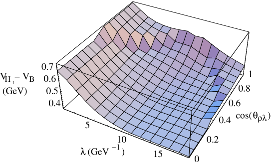
Figure 8: Difference $V_{H_{1}}-V_{B}$ of the hybrid and conventional baryon adiabatic potentials for $\rho=6.2$ GeV^-1, as a function of $\lambda$ and $\theta_{\rho\lambda}$.

The procedure of numerically evaluating the hybrid baryon potential is as follows. For a large set of quark configurations $\{l_{1},l_{2},l_{3}\}$, the Schrödinger equation

$$\left(\frac{1}{2}M_{\mbox{\small eff}}^{\infty}{\bf\dot{r}^{2}}+V_{\mbox{\small J}}\right)\Psi({\bf r})=V(l_{1},l_{2},l_{3})\Psi({\bf r})$$ (42)

is solved variationally for the wave function $\Psi_{B}({\bf r})$ and energy $V_{B}(l_{1},l_{2},l_{3})$ of the ground state of the junction Hamiltonian, as described in section II.6, using the ansatz wave function in Eq. 33. The lowest-lying hybrid ($H_{1}$) baryon potential is found by solving Eq. 42 variationally for the wave function $\Psi_{H_{1}}({\bf r})$ and energy $V_{H_{1}}(l_{1},l_{2},l_{3})$ of the first excited state of the junction Hamiltonian, using the first ansatz wave function in Eq. 34. This corresponds to junction motion in the $QQQ$ plane, and is used because the analytical solutions in section II.5 suggest that the lowest hybrid baryon energy can be described by such junction motion. The minimizations for the baryon and lightest hybrid baryon potentials are carried out independently. It has been checked that the numerical potentials calculated here in the long-string limit agree with the analytic expressions derived in that limit in Sec. II.5, to within 2%.

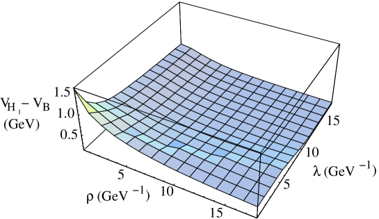
Figure 9: Difference $V_{H_{1}}-V_{B}$ of the hybrid and conventional baryon adiabatic potentials for $\theta_{\rho\lambda}=\pi/2$ as a function of $\rho$ and $\lambda$.

The hybrid baryon adiabatic potential is defined to be

$$\mbox{\={V}}_{H_{1}}(l_{1},l_{2},l_{3}) \equiv \mbox{\={V}}_{B}(l_{1},l_{2},l_{3})+V_{H_{1}}(l_{1},l_{2},l_{3})-V_{B}(l_{1},l_{2},l_{3})$$ (43)

$$= b\sum_{i}l_{i}+V_{H_{1}}(l_{1},l_{2},l_{3})-V_{B}(l_{1},l_{2},l_{3}).$$

Selected numerical results for the difference $V_{H_{1}}-V_{B}$ of the hybrid and conventional baryon adiabatic potentials are plotted in Figures 8–9. In Fig. 8 the potential is plotted with fixed $\rho$ (proportional to the separation of quarks 1 and 2) and variable $\lambda$ (proportional to the separation of the center-of-mass of quarks 1 and 2, and quark 3) and $\theta_{\rho\lambda}$ (the angle between the vectors $\rho$ and $\lambda$), which clearly demonstrates a discontinuity in the derivative when the flux goes from the shape with $\theta_{J}=120^{o}$ to that with $\theta_{J}>120^{o}$. In Figs. 9 and 10 the behavior of $V_{H_{1}}-V_{B}$ and $V_{B}-b\sum_{i}l_{i}$ when $\rho$ and $\lambda$ are orthogonal is plotted against $\rho$ and $\lambda$. It is obvious that both the conventional and hybrid baryon adiabatic potentials increase when $\rho\lambda$ is small, with the hybrid adiabatic potential increasing faster. If the small-oscillations approximation were employed they would tend to infinity as $\rho\lambda\rightarrow 0$. Solving for the energy variationally has softened this behaviour considerably.

The value of $\sqrt{M_{\mbox{\small eff}}^{\infty}\omega_{-}}$ for the baryon is approximately in the range $0.37-0.5$ GeV, while the hybrid baryon is $\approx 0.35-0.48$ GeV.

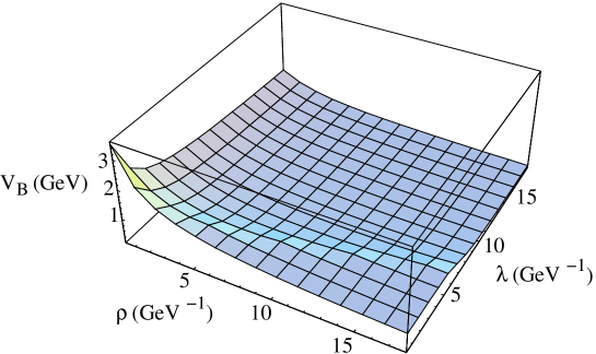
Figure 10: Conventional baryon adiabatic potential without the confining potential, $V_{B}-b\sum_{i}l_{i}$, for $\theta_{\rho\lambda}=\pi/2$, as a function of $\rho$ and $\lambda$.

V.2 Short-distance interactions between the quarks

There are two important configurations of the quarks when considering the Coulomb interactions. These are where two quarks are near to each other and the third is distant (meson-like configurations), and where all three quarks are close to each other. It is possible to focus on the former, because the latter is atypical and contributes little to the energy of the baryon.

In the flux-tube model, in the meson-like configuration a string extends from the distant quark to the other two quarks, i.e. the system looks like a meson with the two nearby quarks in color $\bf\bar{3}$. The reason for this is that the long-distance picture is still appropriate for the distant quark, which means that its color flows along the long string, and must be cancelled by the two nearby quarks. The two nearby quarks are hence in color $\bf\bar{3}$ for both the conventional and hybrid baryon. This implies that the Coulomb interactions between the nearby quarks are attractive, and identical in the conventional and hybrid baryon.

This also has implications for hyperfine contact (spin-spin) interactions, the existence of which has recently been confirmed in lattice QCD karsh , since their form is given by the color representation of the interacting quark pair. The interactions are, therefore, identical for conventional and hybrid baryons. As seen in Table 4 above, the lightest $\Delta$ hybrid baryons have the same quark-spin structure as the ground-state $\Delta$, and both the symmetric and antisymmetric lightest nucleon hybrids have the same quark-spin structure as the ground-state nucleon. This implies that the lightest $\Delta$ hybrid baryons are always heavier than the lightest $N$ hybrids, due to the same hyperfine interaction which makes the $\Delta$ heavier than the nucleon.

VI Numerical mass estimate for low-lying hybrid baryons

The Hamiltonians in Eqs. 41 and 43 are evaluated using the basis of coupled three-dimensional harmonic oscillator wave functions in Eq. 38, expanded up to at least the $N=7$ oscillator level, where $N=2(n_{\rho}+n_{\lambda})+l_{\rho}+l_{\lambda}$. These matrices are subsequently diagonalized to yield the energies. The resulting full wave functions (Eq. 39), which are linear combinations of the harmonic oscillator wave functions, are solutions of the Schrödinger equation for the quark motion in the presence of the usual ${\bar{V}}_{B}$ baryon confining potential and the ${\bar{V}}_{H_{1}}$ hybrid-baryon adiabatic potential. The differences between the energies for the hybrid and the conventional baryon are then added to the experimental mass of the lightest baryon (the nucleon).

It is interesting to determine what sets the scale of the energy difference between the lightest hybrid and conventional baryons in this model. This can be illustrated by examining the analytic solution to the junction Hamiltonian developed above, in the limit of small oscillations and a large number of beads. Equation 31 gives the frequency $\omega_{-}$ of the lowest energy string excitation in terms of the string tension $b$, the effective mass $M^{\infty}_{\rm eff}$ of the junction in the limit of a large number of beads, and the lengths $l_{i}$ of the three lines from the rest position of the junction to the quarks (triads). The effective mass of the junction is, in turn, given in terms of the same quantities and the quark masses $M_{i}$ in Eq. 21. The scale of the energy difference is set by the same quantities in our variational calculations, which do not employ the small oscillations limit.

Consistent values of the string tension and light ($M_{u}=M_{d}$) quark mass are used in evaluating the flux energies, which define the adiabatic potentials in which the quarks move, and in the calculation of the energy of the quarks (and so hybrid and conventional baryon masses) in these potentials. The value of the string tension used is $b=0.18$ GeV², the typical value resulting from lattice gauge theory calculations, which is also used in quark model calculations of hadron masses paton85 . The light quark masses are set to 0.22 GeV, the same value used in Ref. capstick86 , which also uses the relativistic kinetic energy, and Coulomb and hyperfine contact potentials identical to those in the current calculation.

The triad lengths $l_{i}$ are not parameters, as in principle they are evaluated for every set of quark positions in order to find the potential in which the quarks move. Their average size does of course affect the excitation energy of the string, and since this is determined by solving for the motion of the quarks in the confining (and to a lesser extent short-distance) potential, it only depends on the quark masses and string tension.

In the case that the hyperfine contact spin-spin term in Eq. 41 is set to zero, the lightest $L_{q}=0$ states have $M_{H_{1}}-M_{B}=890$ MeV, giving a mass estimate of $M_{H_{1}}=1085+890=1975$ MeV. Here 1085 MeV is the spin-averaged mass of the nucleon and $\Delta$ ground states. Note that this means that all of the lowest-lying $H_{1}$ hybrid states in Table 4 have this mass. Furthermore, the states built on this adiabatic surface with $L_{q}=1$ and $L_{q}=2$ have masses 2340 and 2620 MeV, respectively, showing a considerable cost in energy for orbital excitation of the quarks, comparable to that in the conventional baryons. Similarly, the lightest radial excitation built on this adiabatic surface has mass 2485 MeV, with a position between the $L_{q}=0$ and $L_{q}=2$ states, as is also the case in conventional baryons.

Including the hyperfine contact spin-spin term in Eq. 41 lowers the mass of the quark-spin-1/2 $H_{1}$ hybrid states, which coincide with the lightest $N$ hybrids as outlined in Sec. IV.3, by 110 MeV to 1865 MeV, and raises the mass of the quark-spin-3/2 $H_{1}$ hybrid states, which coincide with the lightest $\Delta$ hybrids, by a similar amount.

These mass predictions depend on the form of the quark Hamiltonian used here (Eq. 41), which has been fit to the baryon spectrum. The parameters which determine the adiabatic potential are the string tension $b$ and the sum of the quark masses $\sum_{i}M_{i}$. In order to conservatively estimate the error in the hybrid masses due to uncertainties in these parameters, a variation of $\delta b/b=\pm 10\%$, and $\delta\sum_{i}M_{i}/\sum_{i}M_{i}=+50\%$ have been considered. These variations change the mass prediction for the lightest hybrid by less than $\pm 100$ MeV.

These mass estimates are substantially higher than other mass estimates in the literature, which are approximately $1.5$ GeV in the bag model bag and $1.5\pm 0.15$ GeV in QCD sum rules QCDsr .

There are two crucial assumptions that were made in the early work on hybrid meson masses in the flux-tube model: the adiabatic motion of quarks and the small-oscillations approximation for bead motion paton85 . It was later shown that when the adiabatic approximation is lifted, the masses go up, and when the small-oscillations approximation is lifted, the masses go down barnes95 . In the present study of hybrid baryons, the adiabatic approximation has been partially lifted by the use of the redefined adiabatic approximation. The small-oscillations approximation has been fully lifted. The effect on the masses of hybrid baryons when the various approximations are lifted is the same as those found for hybrid mesons.

In the numerical simulation described above, with an identical Coulomb interaction in conventional and hybrid baryons, the rms values $\sqrt{\langle\rho^{2}\rangle}=\sqrt{\langle\lambda^{2}\rangle}=2.12$, $2.52$ GeV^-1 are obtained for the baryon and $H_{1}$ hybrid baryon sizes, respectively. The result $\sqrt{\langle\rho^{2}\rangle}=\sqrt{\langle\lambda^{2}\rangle}$ is expected since the spatial parts of the wave functions of the low-lying states are totally symmetric under exchange symmetry. The hybrid baryon is, therefore, 20% larger in size than the conventional baryon.

It is of physical interest to obtain an estimate of the effective junction mass $M_{\mbox{\small eff}}^{\infty}$ in Eq. 21. Taking the average values of $\sqrt{\langle\rho^{2}\rangle}$ and $\sqrt{\langle\lambda^{2}\rangle}$ above with the quarks in an equilateral triangle configuration, with $b=0.18$ GeV², and using Eq. II.5, the junction mass is $M_{\mbox{\small eff}}^{\infty}=0.17$, $0.20$ GeV for the baryon and $H_{1}$ hybrid baryon, respectively. This effective mass is made smaller by the center-of-mass corrections due to the quark motion in Eq. 21. This effective junction mass found in the flux-tube model in the refined adiabatic approximation is very different from the constituent gluon mass of $0.8$ GeV typically employed in constituent gluon models swanson98 , and partially accounts for the higher excitation energy of the hybrid in the present work.

VII Discussion

It is interesting to compare results found here for hybrid baryons to the predictions of the bag model bag . Out of all of the flux-tube model states listed under $H_{1}^{S}$ and $H_{1}^{A}$ in Table 4, only the $N^{2}{\frac{1}{2}}^{+}$, and $N^{2}{\frac{3}{2}}^{+}$ states have the same flavor, quark-spin $S$, total angular momentum and parity as the low-lying hybrid baryons in the bag model. However, restricting to experimentally measurable quantum numbers (flavor, total angular momentum, and parity), only one light-hybrid is different between the flux-tube and bag model predictions. This $J^{P}=5/2^{+}$ state is flavor $\Delta$ in the flux-tube model and flavor $N$ in the bag model, but is amongst the higher-lying states in both models bag .

Looking at quantum numbers alone, the Roper resonance could be regarded as a hybrid baryon candidate in both models. However, our mass estimates do not support this identification, in contrast to some bag model bag and QCD sum rule estimates QCDsr . Both our model and the bag model have seven low-lying hybrid baryons.

One of the disadvantages of hybrid baryons relative to hybrid mesons, multi-quark states and glueballs, is that all possible baryon quantum numbers can be attained by conventional baryons, so there are no “exotic” quantum numbers. However, our low-lying $H_{1}^{A}$ hybrid baryons are “non-relativistic quark model exotic”, since these states have quark-label exchange antisymmetric flux wavefunctions, and so totally antisymmetric space $\times$ spin $\times$ flavor wavefunctions, and states of this nature cannot be constructed in the non-relativistic quark model.

The phenomenology of hybrid baryons has been reviewed recently page02 ; barnes00 and so will not be discussed here.

VIII Conclusions

Significant progress has been made towards building a realistic flux-tube model of (hybrid) baryons. The full multi-bead Hamiltonian is constructed and it is demonstrated that the junction decouples from the beads on the triads to a high degree of accuracy (with the exact and decoupled lowest frequencies differing by at most 2%), so that the lowest-lying hybrid-baryon excitations in the flux-tube model can be associated with the motion of the junction. This simplifies the description of the long distance properties of a low-lying (hybrid) baryon to be that of three quarks and a junction, with the junction connected to each of the quarks via a linear potential. The parameter dependence of the conventional and hybrid-baryon potential is predicted, and can be used as an input in various theoretical approaches.

The quantum numbers of the lightest hybrid baryons in the flux-tube model are given in Table 4, and in the presence of the expected spin-spin interactions between the quarks, the lightest hybrid baryons are four nucleons with $J^{P}=1/2^{+}$, and $3/2^{+}$ and with a mass of 1865$\pm$ 100 MeV.

Acknowledgements

Helpful discussions with T. Barnes, T. Cohen, N. Isgur, G. Karl, R. Lebed, A.V. Nefediev, R. Pack, and E.S. Swanson are gratefully acknowledged. This work is supported by the U.S. Department of Energy under Contracts DE-FG02-86ER40273 (SC) and W-7405-ENG-36 (PRP).

Appendix A Action of the plaquette operator on the junction

It is now shown that the junction can move and leave the string in the ground state of its Y-shaped configuration in first order HLGT perturbation theory, i.e. with the application of a single plaquette operator.

In Fig. 2 the plaquette operator which operates on the junction has the effect of producing a link which is indicated with two arrows on it. The color structure of this link is ${\bf 3}\otimes{\bf 3}={\bf\bar{3}}\oplus{\bf 6}$. A link with color ${\bf 6}$ is not allowed by conservation of color, because its neighboring link is color ${\bf 3}$ flowing in the opposite direction, or color ${\bf\bar{3}}$. However, it would appear that a link with color ${\bf\bar{3}}$ is allowed. The following shows that this is the case.

Figure 11: Enlarged view of the effect of the plaquette operator on the junction in Fig. 2.

An enlargement of the junction region of Fig. 2 is provided in Fig. 11. The creation of a link from spatial positions $A$ to $B$ with color projections $a$ and $b$ respectively, is denoted by $U^{ab}_{AB}$. Denoting by capital letters the spatial positions, and by lowercase letters the color projections, the mathematical expression corresponding to the graph in Fig. 11 is

$$\sum_{dfg_{1}g_{2}g_{3}f^{\prime}ed^{\prime}g^{\prime}}\;\;U^{ad}_{AD}\>U^{dg_{1}}_{DG}\>U^{bg_{2}}_{BG}\>U^{fg_{3}}_{FG}\>U^{cf}_{CF}\>\epsilon_{g_{1}g_{2}g_{3}}\;\;\;U^{f^{\prime}e}_{FE}\>U^{ed^{\prime}}_{ED}\>U^{d^{\prime}g^{\prime}}_{DG}\>U^{g^{\prime}f^{\prime}}_{GF},$$ (44)

where the first term is the initial baryon state and the second term is the plaquette operator. Now contract the two $DG$ links, and the two $FG$ links, using Appendix B of ref. kogut2

$$U^{dg_{1}}_{DG}U^{d^{\prime}g^{\prime}}_{DG} = \frac{1}{2}\sum_{d^{\prime\prime}g^{\prime\prime}}\epsilon_{dd^{\prime}d^{\prime\prime}}\epsilon_{g_{1}g^{\prime}g^{\prime\prime}}U^{g^{\prime\prime}d^{\prime\prime}}_{GD}+$$ (45)

$$\frac{1}{4}\sum_{d^{\prime\prime}d^{\prime\prime\prime}g^{\prime\prime}g^{\prime\prime\prime}}(\delta_{dd^{\prime\prime}}\delta_{d^{\prime}d^{\prime\prime\prime}}+\delta_{dd^{\prime\prime\prime}}\delta_{d^{\prime}d^{\prime\prime}})\;(\delta_{g_{1}g^{\prime\prime}}\delta_{g^{\prime}g^{\prime\prime\prime}}+\delta_{g_{1}g^{\prime\prime\prime}}\delta_{g^{\prime}g^{\prime\prime}})\;U_{DG}^{{\bf 6}\>\{d^{\prime\prime}d^{\prime\prime\prime}\}\>\{g^{\prime\prime}g^{\prime\prime\prime}\}}$$

$$U^{fg_{3}}_{FG}U^{g^{\prime}f^{\prime}}_{GF} = \frac{1}{3}\;\delta_{ff^{\prime}}\delta_{g_{3}g^{\prime}}+2\sum_{f^{\prime\prime}g^{\prime\prime}}\frac{\lambda^{f^{\prime\prime}}_{ff^{\prime}}}{2}\frac{\lambda^{g^{\prime\prime}}_{g_{3}g^{\prime}}}{2}\;U_{FG}^{{\bf 8}\>f^{\prime\prime}g^{\prime\prime}},$$ (46)

where $U^{{\bf 6}}$ and $U^{{\bf 8}}$ refer to sextet and octet links respectively, and $\lambda^{a}$ are the usual Gell-Mann SU(3) matrices. It follows that Eq. 44 equals

$$-\frac{1}{3}\sum_{g^{\prime\prime}fedd^{\prime}d^{\prime\prime}}\;U^{ad}_{AD}\>U^{bg^{\prime\prime}}_{BG}\>U^{g^{\prime\prime}d^{\prime\prime}}_{GD}\>U^{cf}_{CF}\>U^{fe}_{FE}\>U^{ed^{\prime}}_{ED}\>\epsilon_{dd^{\prime}d^{\prime\prime}},$$ (47)

where the ${\bf 6}$ term does not contribute as mentioned above, and the ${\bf 8}$ term is not displayed as it leads to a more complicated topology. Eq. 47 is a mathematical expression which gives a graph similar to Fig. 11, with the junction moved from spatial position $G$ to position $D$, and the links in their usual color triplet state. Hence the application of a single plaquette operator can move the junction and leave the string in its ground state, as promised.

Appendix B Flux-Tube Hamiltonian

The flux-tube Hamiltonian is first derived for the $\theta_{J}=120^{o}$ case, using the coordinate system defined in Eq. 2. The goal is to describe the position of each quark and bead and the junction with respect to an alternative coordinate system with origin at the center of mass ${{\bf R}_{cm}}$ of the entire system.

In this coordinate system the junction is at ${\bf r}_{J}\equiv{\bf r}-{{\bf R}_{cm}}$, where ${\bf r}=(x,y,z)$. The quark positions are

$${\bf r}_{i}\equiv l_{i}(-e^{i}_{y},e^{i}_{x},0)-{{\bf R}_{cm}},$$ (48)

where the $\mbox{\boldmath$e$}^{i}$ are defined in Eq. 10. Bead $n$ on the $i$-th triad is at position

$${\bf r}^{i}_{n}\equiv(-\frac{N_{i}+1-n}{N_{i}+1}e^{i}_{y}l_{i}+\frac{n}{N_{i}+1}x+\xi^{i}_{n}e^{i}_{x},\frac{N_{i}+1-n}{N_{i}+1}e^{i}_{x}l_{i}+\frac{n}{N_{i}+1}y+\xi^{i}_{n}e^{i}_{y},\frac{n}{N_{i}+1}z+z^{i}_{n})-{{\bf R}_{cm}}.$$ (49)

Here $\xi^{i}_{n}$ is the displacement of bead $n$ along the direction $\mbox{\boldmath$e$}^{i}$ which is perpendicular to the $i$-th triad in the QQQ plane (see Fig. 7), and $z^{i}_{n}$ is its displacement perpendicular to the QQQ plane. Note the bead displacements are transverse to the triads on which they lie, and are measured from the line connecting quark $i$ to the (in general displaced) junction. Bead $n=1$ is placed next to the $i$-th quark, and bead $N_{i}$ lies next to the junction.

Requiring that the center of mass is at the origin gives the constraint

$${\bf 0}=m_{J}{\bf r}_{J}+m_{b}\sum_{i=1}^{3}\sum_{n=1}^{N_{i}}{\bf r}^{i}_{n}+\sum_{i=1}^{3}M_{i}{\bf r}_{i},$$ (50)

which can be solved for ${{\bf R}_{cm}}$. The Hamiltonian is

$$H_{\mbox{\small flux}}\equiv\frac{1}{2}m_{J}\dot{{\bf r}}_{J}^{2}+\frac{1}{2}m_{b}\sum_{i=1}^{3}\sum_{n=1}^{N_{i}}(\dot{{\bf r}}^{i}_{n})^{2}+\frac{1}{2}\sum_{i=1}^{3}M_{i}\dot{{\bf r}}_{i}^{2}+\sum_{i=1}^{3}\sum_{n=0}^{N_{i}}|{\bf r}^{i}_{n+1}-{\bf r}^{i}_{n}|,$$ (51)

where the first three terms form the kinetic energy. The last term is the linear potential energy between neighboring beads, where ${\bf r}^{i}_{N_{i}+1}$ is defined as the position of the junction ${\bf r}_{J}$ and ${\bf r}^{i}_{0}$ is defined as the quark position ${\bf r}_{i}$.

The Hamiltonian is now simplified using the redefined adiabatic approximation, where the distances between the quarks remain fixed, concisely stated as $\dot{l}_{i}=0$. The small-oscillations approximation is used to Taylor expand the potential energy in Eq. 51 to yield a function quadratic in the junction and bead position coordinates.

The displacements of the beads within and out of the $QQQ$ plane, given by $\xi^{i}_{n}$ and $z^{i}_{n}$, is expanded in terms of the amplitudes of the $m$-th normal mode of the beads, $q_{\parallel m}^{i}$ and $q_{\perp m}^{i}$, respectively, by

$$\xi^{i}_{n}=\sum_{m=1}^{N_{i}}q_{\parallel m}^{i}\sin\frac{mn\pi}{N_{i}+1}\hskip 28.45274ptz^{i}_{n}=\sum_{m=1}^{N_{i}}q_{\perp m}^{i}\sin\frac{mn\pi}{N_{i}+1}.$$ (52)

The potential energy now becomes diagonal in these normal mode amplitudes $q_{\parallel m}^{i}$, $q_{\perp m}^{i}$ of the beads. Carrying out the necessary algebra yields Eq. 5. As an aside, it is perfectly meaningful in Eq. 5 to put $N_{1}=N_{2}=N_{3}=0$, the case with no beads other than the junction.

For the $\theta_{J}>120^{o}$ case the definition of the coordinates in Eqs. 48–49 remains the same, except that the $\mbox{\boldmath$e$}^{i}$ are given by Eq. 15 and there are no beads on the third triad. Carrying out the necessary algebra yields the Hamiltonian discussed in section II.2.

Appendix C Quark label exchange symmetry for the $\theta_{J}=120^{o}$ case in the small-oscillations approximation

It is now shown, using the explicit definition of ${\mbox{\boldmath$\hat{\eta}$}}_{z}$, that both quark-label exchange symmetric and antisymmetric realizations of ${\mbox{\boldmath$\hat{\eta}$}}_{z}$ are possible. First consider the possibility $\sigma_{z}=1$ in the definition Eq. 25 of ${\mbox{\boldmath$\hat{\eta}$}}_{z}$, so that ${\mbox{\boldmath$\hat{\eta}$}}_{z}$ points along ${\mbox{\boldmath$\rho$}}\times{\mbox{\boldmath$\lambda$}}$. By inserting the expressions for $\rho$ and $\lambda$ in Eq. 23 into ${\mbox{\boldmath$\rho$}}\times{\mbox{\boldmath$\lambda$}}$, it can explicitly be verified that ${\mbox{\boldmath$\rho$}}\times{\mbox{\boldmath$\lambda$}}$ is totally antisymmetric under exchange symmetry. Hence, ${\mbox{\boldmath$\hat{\eta}$}}_{z}$ with $\sigma_{z}=1$ is totally antisymmetric under quark label exchange symmetry.

Another possibility is to choose ${\mbox{\boldmath$\hat{\eta}$}}_{z}$ along the vector

$$\left[\hat{\bf Z}\cdot{{\mbox{\boldmath$\rho$}}}\times{{\mbox{\boldmath$\lambda$}}}\right]{{\mbox{\boldmath$\rho$}}}\times{{\mbox{\boldmath$\lambda$}}},$$ (53)

where $\hat{\bf Z}$ is a space-fixed unit vector (not determined by the quark positions). This is equivalent to choosing

$$\sigma_{z}=\frac{\hat{\bf Z}\cdot{{\mbox{\boldmath$\rho$}}}\times{{\mbox{\boldmath$\lambda$}}}}{|\hat{\bf Z}\cdot{{\mbox{\boldmath$\rho$}}}\times{{\mbox{\boldmath$\lambda$}}}|}$$ (54)

in Eq. 25. This choice of $\sigma_{z}$ obviously yields a totally symmetric ${\mbox{\boldmath$\hat{\eta}$}}_{z}$.

Next consider the quark-label exchange symmetry of ${\mbox{\boldmath$\hat{\eta}$}}_{-}$ and ${\mbox{\boldmath$\hat{\eta}$}}_{-}$ in the $\theta_{J}=120^{o}$ case in the small-oscillations approximation, as defined in Eq. 26. Consider the vectors ${\mbox{\boldmath$\hat{\eta}$}}_{\pm}^{\prime}$, defined by ${\mbox{\boldmath$\hat{\eta}$}}_{\pm}=\sigma_{\pm}{\mbox{\boldmath$\hat{\eta}$}}_{\pm}^{\prime}$. Applying $P_{ij}$ exchanges $l_{i}\leftrightarrow l_{j}$ in Eq. 26, as well as the labels $i$ and $j$ in $\hat{\bf x}$ and $\hat{\bf y}$ in Eq. 2. Under $P_{12}$, it is easy to see that ${\mbox{\boldmath$\hat{\eta}$}}_{\pm}^{\prime}\rightarrow-{\mbox{\boldmath$\hat{\eta}$}}_{\pm}^{\prime}$. Both $P_{13}$ and $P_{23}$ can be shown to lead to ${\mbox{\boldmath$\hat{\eta}$}}_{\pm}^{\prime}\rightarrow\pm{\mbox{\boldmath$\hat{\eta}$}}_{\pm}^{\prime}$, where the sign is dependent on the relative sizes of $l_{1}$, $l_{2}$, and $l_{3}$. For example, under $P_{23}$ one can show that this sign is given by the sign of the expression

$$\sqrt{s(l_{1},l_{2},l_{3})}\pm(\frac{1}{l_{2}}+\frac{1}{l_{3}}-\frac{2}{l_{1}}),$$ (55)

where $s(l_{1},l_{2},l_{3})$ is defined in Eq. 27.

The fact that the ${\mbox{\boldmath$\hat{\eta}$}}_{\pm}^{\prime}$ transform under label exchange into themselves, up to a sign, follows from the observation that the ray in which the ${\mbox{\boldmath$\hat{\eta}$}}_{\pm}^{\prime}$ lie is the physical line of oscillation of the junction in these vibrational modes. Since label exchange does not change the physics, the oscillation should still be in the same ray after label exchange, as found. Since only the ray in which ${\mbox{\boldmath$\hat{\eta}$}}_{\pm}$ lies is physical, the possibility cannot be excluded that the ${\mbox{\boldmath$\hat{\eta}$}}_{\pm}^{\prime}$ are multiplied by a sign $\sigma_{\pm}$ when a standard choice of eigenvectors is constructed, as in Eq. 26. It is possible to show that a consistent set of sign conventions $\sigma_{\pm}$ can be chosen such that the ${\mbox{\boldmath$\hat{\eta}$}}_{\pm}$ are either totally symmetric or antisymmetric under label exchange. Neither choice can be excluded.

It is also possible to show that the signs $\sigma_{-}$, $\sigma_{+}$ and $\sigma_{z}$ are invariant under parity.

References

- (1) T.P. Vrana, S.A. Dytman, and T.S. Lee, Phys. Rept. 328, 181 (2000).
- (2) Z.-P. Li, Phys. Rev. D 44, 2841 (1991); Z.-P. Li, V. Burkert, and Z.-J. Li, Phys. Rev. D 46, 70 (1992).
- (3) P.R. Page, Phys. Lett. B 402, 183 (1997); F.E. Close and P.R. Page, Nucl. Phys. B 443, 233 (1995); Phys. Rev. D 52, 1706 (1995).
- (4) L.S. Kisslinger and Z.-P. Li, Phys. Rev. D 51, 5986 (1995); L.S. Kisslinger, Nucl. Phys. A 629, 30c (1998).
- (5) C.-K. Chow, D. Pirjol, and T.-M. Yan, Phys. Rev. D 59, 056002 (1999).
- (6) T. Barnes and F.E. Close, Phys. Lett. B 123, 89 (1983); E. Golowich, E. Haqq, and G. Karl, Phys. Rev. D 28, 160 (1983); C.E. Carlson and T.H. Hansson, Phys. Lett. B 128, 95 (1983); I. Duck and E. Umland, Phys. Lett. B 128, 221 (1983); C.E. Carlson, Proc. of the Int. Conf. on the Structure of Baryons (October 1995, Santa Fe, NM), eds. B.F. Gibson et al., World Scientific, Singapore, 1996, p. 461.
- (7) H. Hogaasen and J.M. Richard, Phys. Lett. B 134, 520 (1983).
- (8) S. Capstick and N. Isgur, Phys. Rev. D 34, 2809 (1986).
- (9) S. Capstick, Phys. Rev. D 46, 1965 (1992).
- (10) R.A. Arndt, J.M. Ford, and L.D. Roper, Phys. Rev. D 32, 1085 (1984).
- (11) R.E. Cutkosky and S. Wang, Phys. Rev. D 42, 235 (1990).
- (12) J. Speth, O. Krehl, S. Krewald, and C. Hanhart, Nucl. Phys. A 680, 328 (2000).
- (13) N. Isgur and J. Paton, Phys. Rev. D 31, 2910 (1985); Phys. Lett. B 124, 247 (1983); S. Capstick, S. Godfrey, N. Isgur, and J. Paton, Phys. Lett. B 175, 457 (1986); I. Zakout and R. Sever, Z. Phys. C 75, 727 (1997).
- (14) G.S. Bali, Nucl. Phys. Proc. Suppl. 83, 422 (2000); S. Deldar, Nucl. Phys. Proc. Suppl. 83, 440 (2000).
- (15) C. Michael, Proc. of Quark Confinement and the Hadron Spectrum III (Confinement III), (Newport News, VA, 7-12 June 1998), ed. N. Isgur, World Scientific, Singapore, p. 93;
- (16) D.S. Kuzmenko and Yu.A. Simonov, hep-ph/0202277.
- (17) D.E. Kharzeev, Phys. Lett. B 378, 238 (1996); B.Z. Kopeliovich, Phys. Lett. B 446, 321 (1999); ibid. B 381, 325 (1996); S.E. Vance, M. Gyulassy, and X.N. Wang, Phys. Lett. B 443, 45 (1998).
- (18) E.S. Swanson and A.P. Szczepaniak, Phys. Rev. D 59, 014035 (1999).
- (19) K.J. Juge, J. Kuti, and C.J. Morningstar, Nucl. Phys. Proc. Suppl. 63, 543 (1998).
- (20) T.J. Allen, M.G. Olsson, and S. Veseli, Phys. Lett. B 434, 110 (1998).
- (21) P.R. Page, Proc. of The Physics of Excited Nucleons (NSTAR2000), (Newport News, VA, 16-19 Feb. 2000), eds. V.D. Burkert, L. Elouadrhiri, J.J. Kelly, and R.C. Minehart, World Scientific, Singapore, 2001, p. 171, nucl-th/0004053.
- (22) S. Capstick and P. R. Page, Phys. Rev. D 60, 111501 (1999).
- (23) J. Merlin and J. Paton, Jour. Phys. G 11, 439 (1985). G.S. Bali, Fizika B 8, 229 (1998); T.T. Takahashi, H. Matsufuru, Y. Nemoto, and H. Suganuma, Phys. Rev. Lett. 86, 18 (2001); Proc. of Int. Symp. on Hadron and Nuclei (Feb. 2001, Seoul, Korea), published by Institute of Physics and Applied Phyics (2001), ed. Dr. T.K. Choi, p. 341; T.T. Takahashi, H. Matsufuru, Y. Nemoto, H. Suganuma, and T. Umeda, Nucl. Phys. Proc. Suppl. 94, 554 (2001).
- (24) M. Luscher, Nucl. Phys. B 180, 317 (1981).
- (25) C. Michael and P. Stephenson, Phys. Rev. D 50, 4634 (1994).
- (26) Yu.S. Kalashnikova and A.V. Nefediev, Phys. Atom. Nucl. 60, 1333 (1997); Phys. Lett. B 367, 265 (1996).
- (27) K.J. Juge, J. Kuti, and C.J. Morningstar, Nucl. Phys. Proc. Suppl. 63, 326 (1998); C.J. Morningstar, Proc. of the Int. Conf. on Hadron Spectroscopy (Hadron’97), (Upton, NY, 25-30 Aug. 1997), eds. S.-U. Chung and H.J. Willutzki, American Institute of Physics, 1998, p. 136; C.J. Morningstar, Proc. of Quark Confinement and the Hadron Spectrum III (Confinement III), (Newport News, VA, 7-12 June 1998), ed. N. Isgur, World Scientific, Singapore, p. 179, hep-lat/9809015.
- (28) J. Kogut and L. Susskind, Phys. Rev. D 11, 395 (1975).
- (29) See, for example, S. Capstick, Proc. of Hadron Spectroscopy and the Confinement Problem (Swansea, UK, 27 June - 8 July 1995), ed. D.V. Bugg, NATO ASI Series B: Vol. 353, Plenum Press, 1996, p. 311.
- (30) M. Hess, F. Karsch, E. Laermann, and I. Wetzorke, Phys. Rev. D 58, 111502 (1999).
- (31) T. Barnes, F.E. Close, and E.S. Swanson, Phys. Rev. D 52, 5242 (1995).
- (32) P.R. Page, Proc. of the 9th Int. Conf. on the Structure of Baryons (Baryons 2002), (3-8 March, 2002, Newport News, VA), nucl-th/0204031.
- (33) T. Barnes, contribution to the COSY Workshop on Baryon Excitations (May 2000, Jülich, Germany), nucl-th/0009011.
- (34) J. Kogut, D.K. Sinclair and L. Susskind, Nucl. Phys. B 114, 199 (1976).