On the Surface Structure of Strange Superheavy Nuclei

Abstract

Bound, strange, neutral superheavy nuclei, stable against strong decay, may exist. A model effective field theory calculation of the surface energy and density of such systems is carried out assuming vector meson couplings to conserved currents and scalar couplings fit to data where it exists. The non-linear relativistic mean field equations are solved assuming local density baryon sources. The approach is calibrated through a successful calculation of the known nuclear surface tension.

I Introduction

An inspection of the semiempirical mass formula (SEMF) reveals that the single largest limiting factor in the creation of very large nuclei is the Coulomb repulsion. One way to overcome this barrier is to include hyperons in nuclei Schaffner et al. (1993); Schaffner-Bielich and Gal (2000); Stoks and Lee (1999). Consider the hyperons $\Lambda^{0}$, $\Sigma^{(\pm,0)}$, and $\Xi^{(-,0)}$. The lightest hyperon, the $\Lambda$, has a negative binding energy in nuclear matter Gal et al. (1988) and decays weakly into nonstrange matter. The $\Sigma$’s appear to have a repulsive nuclear potential Gal et al. (1995); Bart, et al. (1999); Dabrowski (1999). Next in mass are the $\Xi$’s; experimental evidence suggests that the binding energy of a single $\Xi$ in nuclear matter is negative Gal (2001); Fukuda, et al. (1998); Khaustov, et al. (2000). In addition, the reaction $2\Lambda\rightarrow N+\Xi$ becomes energetically favorable for some critical number of $\Lambda$’s in the nuclear medium Schaffner et al. (1993). As a result, we expect that for large systems the addition of $\Lambda$’s and $\Xi$’s is desirable, but the inclusion of $\Sigma$’s would have little or no positive effect. Therefore we consider matter composed solely of p, n, $\Lambda$, $\Xi^{0}$, and $\Xi^{-}$. The inclusion of the $\Xi^{-}$’s offsets the Coulomb repulsion of the protons; this potentially allows for the creation of arbitrarily large nuclei by diminishing the importance of the Coulomb term in the SEMF. To minimize the effect of the Coulomb term we investigate this class of nuclei such that $\mathrm{Q}=0$. Due to the fact that these nuclei are stable against strong decay, they consequently decay on weak interaction timescales enhancing the potential for their detection. The purpose of this paper is to model the surface structure, and acquire the surface energy from the calculated SEMF, for this class of nuclei.

To accomplish this, we must solve the nuclear many-body problem. Using quantum hadrodynamics (QHD), we construct an effective lagrangian density invariant under $SU(2)_{L}\bigotimes SU(2)_{R}$ symmetry using hadrons as degrees of freedom Furnstahl et al. (1996); Walecka (1995). Isodoublet baryon fields, $\psi$, are coupled to the meson fields $\phi$, V, $\rho$, and $\pi$; the meson fields correspond to an isoscalar, Lorentz scalar and vector, and an isovector, vector and pseudoscalar, fields respectively Serot and Walecka (1997). In the relativistic mean field limit, the meson fields become classical fields and the sources become expectation values. The pions have no mean fields in a spherically symmetric system. Then the lagrangian density is converted into a hamiltonian density; since it is explicitly time independent the hamiltonian density is equivalent to the energy density. The baryon mass is determined by solving the scalar field equation self-consistently at each point Walecka (1995); Serot and Walecka (1986). The coupling constants are fit to reproduce experimental values of various ordinary nuclei; specifically the parameter sets NLC and Q1, which include nonlinear scalar couplings, are used Serot and Walecka (1997); Furnstahl et al. (1996). This theory, when solved in the relativistic Hartree approximation, has had great success in predicting the bulk properties and shell structure in ordinary nuclei Furnstahl et al. (1997a); Furnstahl et al. (1996).

To investigate the structure of the many-particle superheavy nuclei of interest here, we directly use the approach of density functional theory (DFT). DFT tells us that the exact ground-state density is acquired by minimizing the energy functional Serot and Walecka (1997); Kohn (1999). The effective lagrangian discussed above provides a lowest order density functional. The scalar and vector fields here play the role of relativistic Kohn-Sham potentials Kohn (1999); Serot and Walecka (2000). In order to calibrate our approach, we calculate the ground-state densities of ordinary finite nuclei with N = Z. To model finite nuclei we must add spherically symmetric spatial variations of the meson fields to the lagrangian density. The source terms are evaluated using a local density approximation; at every point within the nucleus the baryons are assumed to be a local Fermi gas with states filled up to $k_{F}$. We acquire the scalar mean field equation by minimizing the energy functional with respect to the scalar field; a similar approach yields the vector mean field equation Serot and Walecka (1986).

The nonlinear scalar field equation is solved as a finite difference equation utilizing a shooting method. The boundary conditions are determined by assuming the baryon density vanishes at the surface and solving the linear scalar field equation outside Serot and Walecka (1986). However, these boundary conditions are exact only in the linear case; a correction term must be added to compensate for the effects of nonlinear terms in the scalar field equation. The total energy is minimized with respect to the local Fermi wave number, while keeping fixed the baryon number, B. The constraint of fixed B is incorporated with a Lagrange multiplier, which is the chemical potential. The resulting constraint equation states that the chemical potential must be constant throughout the nucleus Serot and Walecka (1986). This approach is more sophisticated than a simple Thomas-Fermi method because we self-consistently solve for the source terms at each point. With the calculated binding energy and baryon number for finite nuclei, we fit the first two terms in the SEMF, the bulk and surface energies, for nuclear matter. These are in good agreement with the known experimental values Walecka (1995), thereby validating our approach.

Now we add in hyperons; however, existing experimental data requires that some assumptions be made. First, we couple universally to the conserved baryon and isovector currents. Second, a different scalar coupling is used for each baryon. The scalar coupling for the $\Lambda$’s is fit such that the binding energy of a single $\Lambda$ in nuclear matter is -28 MeV Gal et al. (1988). However the binding energy of a single $\Xi$ is relatively uncertain, values appearing in the literature range from -40 to -14 MeV. Recent experiments with light nuclei suggest that the value lies on the less bound side of this range Fukuda, et al. (1998); Khaustov, et al. (2000); however, it may be more deeply bound for heavy nuclei Yamamoto et al. (1994). As a result, a number of values for the $\Xi$ scalar coupling are investigated. Third, we continue to utilize the parameter sets for ordinary nuclear matter, NLC and Q1, to generate the nucleon and non-linear scalar couplings.

The addition of new baryons in the theory only requires the inclusion of new source terms in the effective lagrangian density. We investigate a specific sector of the theory by imposing the restrictions $\mathrm{Q}=0$ and $\mathrm{|S|/B}=1$, where S is the total strangeness. We also assume an average cascade mass. Note that the minimum binding energy always occurs such that there are equal numbers of n and p (and consequently equal numbers of $\Xi^{0}$ and $\Xi^{-}$); therefore the symmetry term in the SEMF is rendered irrelevant. Since there is only one chemical potential, the reactions $2\Lambda\leftrightarrow N+\Xi$ and $n+\Xi^{0}\leftrightarrow p+\Xi^{-}$ are in equilibrium. Again, using DFT to model finite nuclei, we now investigate the role of the first two terms in the calculated SEMF. Also, by determining the baryon density, we acquire the structure of the surface.

At $T=0$ and normal nuclear densities, the mass difference between strange and nonstrange quarks is less then the Fermi energy of massless nonstrange quarks. This opened the possibility that strange quark matter composed of u, d, and s quarks might be stable against strong decay and perhaps even absolutely stable Witten (1984); Farhi and Jaffe (1984). These systems are characterized by small charge fraction $\mathrm{Q/B}\sim 0$ and large strangeness fraction $\mathrm{|S|/B}\sim 1$. The plausibility of bound strange matter has also been explored in the hadronic sector. Theoretical investigations of multiple $\Lambda$ hypernuclei indicate that they are bound and stable against strong decay. These studies produced systems with binding energies as low as -9 MeV corresponding to $\mathrm{|S|/B}\sim 0.2$ Mares and Zofka (1993); Rufa et al. (1990); Barranco et al. (1991); Lanskoy and Tretyakova (1992); Schulze et al. (1998).

Gal et. al. suggested that discussions of matter composed of n, p, and $\Lambda$ must also include $\Xi^{0}$ and $\Xi^{-}$ due to the fact that the reaction $2\Lambda\rightarrow N+\Xi$ is energetically favorable for some critical number of $\Lambda$’s in the nuclear medium Schaffner et al. (1993). They investigated possible configurations of bulk matter in the relativistic mean field approach, suggesting binding energies per baryon as low as -25 MeV with a large strangeness fraction; finite nuclear calculations were also preformed Schaffner-Bielich and Gal (2000); Gal et al. (1995); Gal and Dover (1995); Schaffner et al. (1994). In addition, Gal et. al. fit to a generalized SEMF using a Fermi gas model Gal and Dover (1993); Balberg et al. (1994). Extrapolating from the ordinary SEMF they estimate the bulk and symmetry terms, while leaving the Coulomb term unchanged. The surface energy is scaled as inversely proportional to the average baryon mass, yielding a value of 15 MeV. Stoks and Lee challenged these findings using a many-body theory with baryon-baryon potential models. These potentials were developed using an $SU(3)$ extension of the Nijmegen soft-core potentials Stoks et al. (1999); Stoks and Rijken (1999); Halderson (1999); Rijken (1998). In contrast, the latter found that this type of matter is only slightly bound, $\mathrm{E/B}\sim-3$ MeV or less Stoks and Lee (1999); Vidana et al. (2000). A quark-meson coupling model produced a minimum binding energy of -24.4 MeV with $\mathrm{|S|/B}\sim 1.38$ Wang et al. (1999). The effect of adding hyperons has also been explored in application to neutron stars Balberg and Gal (1997); Banik and Bandyopadhyay (2000); Baldo et al. (2000); Glendenning (1997).

In this paper we first construct the effective lagrangian of the theory following the methodology of Furnstahl, Serot, and Tang Serot and Walecka (1997); Furnstahl et al. (1996); Furnstahl et al. (1997b). For ordinary nuclear matter, we model both infinite matter and finite nuclei of various radii using QHD. Initially, it was assumed that, because of the relatively large value of vector meson mass, the derivatives of the vector field were negligible Serot and Walecka (1986); however, iteration on the vector field produces a significant effect on the calculation. Also, a correction to the boundary condition is required to account for the nonlinearities in the scalar field equation. From this calculation, we acquire the baryon density and scalar field for ordinary finite nuclei; this provides a picture of the size and shape of the surface. Then the surface energy is extracted by fitting to the SEMF. The approach is successfully calibrated by comparing this result to the experimentally obtained values. Next this system is extended to cascade-nucleon matter, composed of p, n, $\Xi^{0}$, and $\Xi^{-}$, subject to the constraints $\mathrm{Q}=0$ and $\mathrm{|S|/B}=1$. However, due to the uncertainty in the binding of a single cascade in nuclear matter, we examine a range of values for the $\Xi$ scalar coupling. Again, by calculating finite systems, the bulk and surface terms are extracted from the SEMF. $\Lambda$’s are then added to the cascade-nucleon matter, with the $\Lambda$ scalar coupling fit to experiment. The bulk quantities change little, however, from the cascade-nucleon case. An investigation of possible hyperon-hyperon interaction is conducted by coupling a $\Phi$ meson to the conserved strangeness current; we allow the $\Phi$ coupling to increase until the many-body system is no longer bound in order to find the maximum allowable value of this coupling.

The organization of this paper is as follows. In section 2, the effective lagrangian is constructed and the systems of equations are derived. In section 3, we present the methodologies used to solve these systems described in section 2. In section 4, the results for nuclear and hyperon-nucleon matter are discussed.

II Theory

Following the QHD approach of Furnstahl et. al. Furnstahl et al. (1996); Furnstahl et al. (1997b); Serot and Walecka (1997), we construct an effective lagrangian density using hadronic degrees of freedom that remains invariant under $SU(2)_{L}\bigotimes SU(2)_{R}$ symmetry. We will use this lagrangian density to model both infinite and finite systems; to start with only systems of nucleons with $N=Z$, which we refer to as nucleon matter, are considered. The full lagrangian density (with $\hbar=c=1$) is given by

$${\cal{L}}(x_{\mu}) = -\bar{\psi}\left[\gamma_{\mu}\left(\frac{\partial}{\partial x_{\mu}}-ig_{v}V_{\mu}\right)+M-g_{s}\phi\right]\psi$$ (1)

$$-\frac{1}{2}\left[\left(\frac{\partial\phi}{\partial x_{\mu}}\right)^{2}+m_{s}^{2}\phi^{2}\right]-\frac{1}{4}F_{\mu\nu}F_{\mu\nu}$$

$$-\frac{1}{2}m_{v}^{2}V_{\mu}^{2}-\frac{\kappa}{3!}\phi^{3}-\frac{\lambda}{4!}\phi^{4}$$

Here $\psi=\left(\begin{array}[]{c}p\\ n\end{array}\right)$ is the isodoublet baryon field, $\gamma_{\mu}=(i\vec{\alpha}\beta,\beta)$ are the gamma matrices, and $\mu,\nu=1,\ldots 4$. The conventions of Walecka (1995) are used. The Lorentz scalar meson field, $\phi$, is coupled to the scalar density $\bar{\psi}\psi$ and $V_{\mu}$, the Lorentz vector meson field, is coupled to the conserved baryon current $i\bar{\psi}\gamma_{\mu}\psi$; their respective coupling constants are $g_{s}$ and $g_{v}$. The masses of the nucleon, scalar, and vector fields are denoted by $M$, $m_{s}$, and $m_{v}$ respectively. $\kappa$ and $\lambda$ are constants that determine the strength of the nonlinear scalar couplings. The field tensor is defined as

$$F_{\mu\nu}=\frac{\partial V_{\nu}}{\partial x_{\mu}}-\frac{\partial V_{\mu}}{\partial x_{\nu}}$$ (2)

Notice the $\rho$-meson terms in Eq. (1) have been suppressed. The source term contributed by the $\rho$-meson depends on $N-Z$, which vanishes for the systems under consideration. We now employ relativistic mean field theory (RMFT). In this case the meson fields are replaced by their classical, or mean fields

$$\phi(x_{\mu}) \longrightarrow \phi_{0}(r)$$ (3)

$$V_{\mu}(x_{\mu}) \longrightarrow i\delta_{\mu 4}V_{0}(r)$$ (4)

which are time-independent. For the purposes of this paper, we restrict ourselves to spherical symmetry. The source terms are now replaced by their expectation values. In DFT, the classical fields play the role of Kohn-Sham potentials Serot and Walecka (1997, 2000). Incorporating both Eq. (2) and RMFT, our lagrangian density becomes

$${\cal{L}}(x_{\mu}) = -\bar{\psi}\left(\gamma_{\mu}\frac{\partial}{\partial x_{\mu}}+M^{*}\right)\psi-g_{v}V_{0}\psi^{\dagger}\psi$$ (5)

$$+\frac{1}{2}[(\nabla V_{0})^{2}+m_{v}^{2}V_{0}^{2}]-\frac{1}{2}[(\nabla\phi_{0})^{2}+m_{s}^{2}\phi_{0}^{2}]$$

$$-\frac{\kappa}{3!}\phi_{0}^{3}-\frac{\lambda}{4!}\phi_{0}^{4}$$

where the effective mass is defined as

$$M^{*}\equiv M-g_{s}\phi_{0}$$ (6)

Now the hamiltonian density is given by

$${\cal{H}}(x_{\mu}) = \Pi\frac{\partial\psi}{\partial t}-{\cal{L}}$$ (7)

$$= \psi^{\dagger}\frac{\partial\psi}{\partial t}+\bar{\psi}\left(\gamma_{\mu}\frac{\partial}{\partial x_{\mu}}+M^{*}\right)\psi+g_{v}\rho_{B}V_{0}$$

$$-\frac{1}{2}[(\nabla V_{0})^{2}+m_{v}^{2}V_{0}^{2}]+\frac{1}{2}[(\nabla\phi_{0})^{2}+m_{s}^{2}\phi_{0}^{2}]$$

$$+\frac{\kappa}{3!}\phi_{0}^{3}+\frac{\lambda}{4!}\phi_{0}^{4}$$

where $\rho_{B}=\psi^{\dagger}\psi$ is the baryon density and the canonical momentum density is

$$\Pi=\frac{\partial{\cal{L}}}{\partial(\partial\psi/\partial t)}=i\psi^{\dagger}$$ (8)

If one assumes that a nucleus is a local Fermi gas filled up to some $k_{F}(r)$ at every point, the source terms take the form

$$\rho_{B}(r)=\langle\psi^{\dagger}\psi\rangle=\frac{\gamma}{(2\pi)^{3}}\int_{0}^{k_{F}(r)}d^{3}k$$ (9)

$$\langle\psi^{\dagger}(\vec{\alpha}\cdot\vec{p}+\beta M^{*})\psi\rangle=\frac{\gamma}{(2\pi)^{3}}\int_{0}^{k_{F}(r)}(k^{2}+M^{*2})^{1/2}d^{3}k$$ (10)

where $\vec{p}=-i\nabla$ and $\gamma$ is a degeneracy factor. Since the hamiltonian density is explicitly time-independent, it is equivalent to the energy density (with $\gamma=4$ for nucleon matter)

$${\cal{E}}(r) = \frac{1}{2}[(\nabla\phi_{0})^{2}+m_{s}^{2}\phi_{0}^{2}]-\frac{1}{2}[(\nabla V_{0})^{2}+m_{v}^{2}V_{0}^{2}]$$ (11)

$$+g_{v}\rho_{B}V_{0}+\frac{\kappa}{3!}\phi_{0}^{3}+\frac{\lambda}{4!}\phi_{0}^{4}$$

$$+\frac{4}{(2\pi)^{3}}\int_{0}^{k_{F}}(k^{2}+M^{*2})^{1/2}d^{3}k$$

The total energy and baryon number are

$$E=\int{\cal{E}}(r)d^{3}r;\>\;\;\;B=\int\rho_{B}(r)d^{3}r$$ (12)

The energy density above provides a lowest order density functional. DFT tells us that minimizing the exact energy functional yields the exact ground-state density.

To conduct infinite nucleon matter calculations, we neglect spatial variations in the meson fields; the resulting energy density is

$${\cal{E}} = \frac{1}{2}m_{s}^{2}\phi_{0}^{2}+\frac{\kappa}{3!}\phi_{0}^{3}+\frac{\lambda}{4!}\phi_{0}^{4}+g_{v}\rho_{B}V_{0}-\frac{1}{2}m_{v}^{2}V_{0}^{2}$$ (13)

$$+\frac{4}{(2\pi)^{3}}\int_{0}^{k_{F}}(k^{2}+M^{*2})^{1/2}d^{3}k$$

By minimizing the energy functional with respect to the scalar field, the scalar mean field equation is determined. The vector mean field equation is similarly derived as an extremum of the energy functional. These equations are

$$\phi_{0}+\frac{\kappa}{2m_{s}^{2}}\phi_{0}^{2} + \frac{\lambda}{6m_{s}^{2}}\phi_{0}^{3}=\frac{g_{s}}{m_{s}^{2}}\rho_{s}$$ (14)

$$V_{0} = \frac{g_{v}}{m_{v}^{2}}\rho_{B}$$ (15)

where the scalar density is given by

$$\rho_{s}=\frac{4}{(2\pi)^{3}}\int_{0}^{k_{F}}d^{3}k\frac{M^{*}}{(k^{2}+M^{*2})^{1/2}}$$ (16)

The solution to these equations is discussed in section 3.

We now turn our attention to finite nucleon systems. We retain the spherically symmetric spatial variations in the meson fields and therefore require the full energy density in Eq. (11). The meson field equations, acquired in the same manner as above, are

$$(\nabla^{2}-m_{s}^{2})\phi_{0}-\frac{\kappa}{2}\phi_{0}^{2} - \frac{\lambda}{6}\phi_{0}^{3}=-g_{s}\rho_{s}$$ (17)

$$(\nabla^{2}-m_{v}^{2})V_{0} = -g_{v}\rho_{B}$$ (18)

Note that for spherically symmetric systems, the laplacian becomes

$$\nabla^{2}=\frac{\partial^{2}}{\partial r^{2}}+\frac{2}{r}\frac{\partial}{\partial r}$$ (19)

Using a Green’s function, the solution to Eq. (18) is

$$g_{v}V_{0} = \frac{g_{v}^{2}}{4\pi}\int d^{3}y\rho_{B}(\vec{y})\frac{e^{-m_{v}|\vec{x}-\vec{y}|}}{|\vec{x}-\vec{y}|}$$ (20)

$$= \frac{g_{v}^{2}}{xm_{v}}\int ydy\rho_{B}(y)\sinh(m_{v}x_{\scriptscriptstyle<})e^{-m_{v}x_{\scriptscriptstyle>}}$$ (21)

where the angular dependence has now been integrated out. Since the contribution of the laplacian in Eq. (18) is small compared with that of the vector meson mass, to a first approximation it can be neglected Serot and Walecka (1986); Walecka (1995),

$$g_{v}V_{0}=\frac{g_{v}^{2}}{m_{v}^{2}}\rho_{B}$$ (22)

However, the omitted term produces a small, but important, contribution to the vector field; this can have a significant effect on the total energy and baryon number. It is then convenient to express the vector field as

$$g_{v}V_{0}=\frac{g_{v}^{2}}{m_{v}^{2}}\rho_{B}+\delta W_{0}$$ (23)

with $\delta W_{0}\equiv g_{v}\delta V_{0}$. Substituting this in Eq. (21) and rearranging, one obtains an explicit expression for $\delta W_{0}$ in terms of the baryon density

$$\delta W_{0}(r)=\frac{g_{v}^{2}}{4\pi}\int d^{3}y\rho_{B}(\vec{y})\frac{e^{-m_{v}|\vec{x}-\vec{y}|}}{|\vec{x}-\vec{y}|}-\frac{g_{v}^{2}}{m_{v}^{2}}\rho_{B}(r)$$ (24)

Minimization of the total energy with respect to the local Fermi wave number now yields the ground state of the system. A Lagrange multiplier is used to incorporate the constraint of fixed B such that

$$\delta E(k_{F},\phi_{0},V_{0})-\mu\delta B(k_{F})=0$$ (25)

Since the variations of the energy density with respect to both the scalar and vector field vanish, they can be held constant in the variation of $k_{F}$, the result of which is the constraint equation

$$\mu=g_{v}V_{0}(r)+[k_{F}^{2}(r)+M^{*2}(r)]^{1/2}$$ (26)

where the Lagrange multiplier, $\mu$, is the chemical potential and is constant throughout the nucleus.

On the surface $r=r_{0}$, the baryon density vanishes. The constraint equation at the surface then yields the first boundary condition

$$M^{*}(r_{0})=\mu-\delta W_{0}(r_{0})$$ (27)

where Eq. (23) has now been employed.

To determine the second boundary condition, consider the solution to the linear homogeneous scalar field equation

$$\phi_{0}=\phi_{c}\frac{e^{-(r-r_{0})m_{s}}}{r/r_{0}}$$ (28)

The constant $g_{s}\phi_{c}=M-\mu+\delta W_{0}(r_{0})$ is determined at the surface. Differentiating Eq. (28) with respect to $r$ and then evaluating at the surface, we acquire the second boundary condition

$$\left[\frac{\partial M^{*}(r)}{\partial r}\right]_{r_{0}}=[M+\delta W_{0}(r_{0})-\mu]\left(\frac{1+m_{s}r_{0}}{r_{0}}\right)(1+\epsilon)$$ (29)

The solution to the scalar field equation in Eq. (28) no longer holds when the nonlinear terms are included; therefore, a small correction $\epsilon$ has been included to compensate. In the nonlinear case, the scalar field equation is integrated outward from $r_{0}$, and $\epsilon$ in Eq. (29) is varied until the solution vanishes for large $r$.

The calculated binding energy and baryon number of a series of nuclei with different radii can be fit with a SEMF of the form

$$\frac{E}{B}=a_{1}+a_{2}B^{-1/3}$$ (30)

where only the bulk and surface terms have been retained. The bulk constant, $a_{1}$, is determined by the binding energy of infinite nuclear matter. Then, after calculating a number of finite nuclei, the surface energy, $a_{2}$, can be obtained by plotting the calculated energies per baryon against the calculated values of $B^{-1/3}$. The results of numerical methods for these finite systems are discussed in later sections.

We now extend our theory to consider systems of nucleons and hyperons. First we investigate matter composed of n, p, $\Xi^{0}$, and $\Xi^{-}$, subject to the conditions

$$Q=0$$ (31)

$$|S|/B=1$$ (32)

where $Q$ and $S$ are the total charge and strangeness respectively. These systems shall be subsequently referred to as cascade-nucleon ($\Xi N$) matter. Equation (31) restricts the system to equal numbers of p and $\Xi^{-}$; similarly, Eq. (32) forces the numbers of n and $\Xi^{-}$ to be equal. Therefore the system is now characterized by two Fermi wave numbers, $k_{Fp}$ and $k_{Fn}$. For simplicity we employ an average cascade mass $M_{\Xi}=(M_{\Xi^{0}}+M_{\Xi^{-}})/2$. Since the energy density is now symmetric under the interchange of $k_{Fp}$ and $k_{Fn}$, the minimum binding energy always occurs such that $k_{Fp}=k_{Fn}$. As a result, we can further restrict this system to a single Fermi wave number, $k_{F}$. It is a consequence of these arguments that equilibrium is imposed upon the reaction

$$n+\Xi^{0}\rightleftharpoons p+\Xi^{-}$$ (33)

and the system is described by only one chemical potential. Again we mention that the $\rho$-mesons do not contribute here for similar reasons to the nucleon case.

Next, we must make some assumptions about the cascade couplings. Since the baryon current is conserved, the vector coupling is taken to be universal, $g_{v}=g_{v\Xi}$. However, an independent scalar coupling for the cascades, $g_{s\Xi}$, is assumed.

Consider the case of infinite $\Xi N$ matter. The addition of hyperons to the theory requires only the addition of new source terms. A source term of the form

$$\delta{\cal{E}}=\frac{\gamma}{(2\pi)^{3}}\int_{0}^{k_{F}}(k^{2}+M_{\Xi}^{*2})^{1/2}d^{3}k$$ (34)

is added to the energy density in Eq. (13) where

$$M_{\Xi}^{*}=M_{\Xi}-g_{s\Xi}\phi_{0}$$ (35)

In addition, a new term is included in the baryon density

$$\delta\rho_{B}=\frac{\gamma}{(2\pi)^{3}}\int_{0}^{k_{F}}d^{3}k$$ (36)

Here $\gamma=4$ for ($\Xi^{0}$,$\Xi^{-}$) with spin up and down. Except for the additional source terms, the meson field equations remain unchanged. The new term added to the source in the scalar field Eq. (14) is

$$\delta\rho_{s}=\frac{4s}{(2\pi)^{3}}\int_{0}^{k_{F}}d^{3}k\frac{M_{\Xi}^{*}}{(k^{2}+M_{\Xi}^{*2})^{1/2}}$$ (37)

where

$$s\equiv g_{s\Xi}/g_{s}$$ (38)

Equation (36) is incorporated into the source in the vector field Eq. (15). The solution to these equations is again discussed in section 3.

We now examine the case of finite $\Xi N$ matter. The source terms in Eqs. (34) and (36) are incorporated into the energy density in Eq. (11). Next the terms in Eqs. (37) and (36) are added to meson field equations in Eqs. (17) and (18) respectively. Then a new constraint equation is produced in the same manner as before

$$\mu=g_{v}V_{0}+\frac{1}{2}[(k_{F}^{2}+M^{*2})^{1/2}+(k_{F}^{2}+M_{\Xi}^{*2})^{1/2}]$$ (39)

Similarly, the boundary conditions are now

$$M^{*}(r_{0})=\frac{1}{1+s}[2\mu-2\delta W_{0}(r_{0})-M_{\Xi}+sM]$$ (40)

$$\left[\frac{\partial M^{*}(r)}{\partial r}\right]_{r_{0}} = \frac{1}{1+s}[2\delta W_{0}(r_{0})-2\mu+M_{\Xi}$$ (41)

$$+M]\left(\frac{1+m_{s}r_{0}}{r_{0}}\right)(1+\epsilon)$$

Consider again the SEMF in Eq. (30). The conditions imposed on $\Xi N$ matter in Eqs. (31) and (32) now justify the elimination of the Coulomb and symmetry terms. Then $a_{1}$ is taken to be the binding energy of infinite $\Xi N$ matter; next, proceeding as before, the surface energy, $a_{2}$, can be extracted.

Finally, we investigate a class of matter in which $\Lambda$’s are added to the $\Xi N$ matter described above. These systems are referred to as lambda-cascade-nucleon ($\Lambda\Xi N$) matter. The previous restrictions do not relate the number of $\Lambda$’s to the number of $N$’s and $\Xi$’s; therefore a second Fermi wave number, $k_{F\Lambda}$, is needed. Again the vector coupling is taken to be universal and an independent scalar coupling, $g_{s\Lambda}$, is employed. Now equilibrium is imposed on the reactions

$$n+\Xi^{0} \rightleftharpoons \Lambda+\Lambda$$ (42)

$$p+\Xi^{-} \rightleftharpoons \Lambda+\Lambda$$ (43)

as well as on Eq. (33). As before, the system is then characterized by a single chemical potential. The source terms required for the inclusion of $\Lambda$’s in both infinite and finite $\Xi N$ matter are

$$\delta{\cal{E}}=\frac{2}{(2\pi)^{3}}\int_{0}^{k_{F\Lambda}}(k^{2}+M_{\Lambda}^{*2})^{1/2}d^{3}k$$ (44)

$$\delta\rho_{B}=\frac{2}{(2\pi)^{3}}\int_{0}^{k_{F\Lambda}}d^{3}k$$ (45)

$$\delta\rho_{s}=\frac{2t}{(2\pi)^{3}}\int_{0}^{k_{F\Lambda}}d^{3}k\frac{M_{\Lambda}^{*}}{(k^{2}+M_{\Lambda}^{*2})^{1/2}}$$ (46)

where

$$M^{*}_{\Lambda}=M_{\Lambda}-g_{s\Lambda}\phi_{0}$$ (47)

and

$$t\equiv g_{s\Lambda}/g_{s}$$ (48)

In the case of finite $\Lambda\Xi N$ matter, there are now two constraint equations

$$\mu=g_{v}V_{0}+\frac{1}{2}[(k_{F}^{2}+M^{*2})^{1/2}+(k_{F}^{2}+M_{\Xi}^{*2})^{1/2}]$$ (49)

$$\mu=g_{v}V_{0}+(k_{F\Lambda}^{2}+M_{\Lambda}^{*2})^{1/2}$$ (50)

The $\Lambda$ density begins interior to the surface $r_{0}$; this allows the $\Xi N$ boundary conditions to be used in the $\Lambda\Xi N$ case.

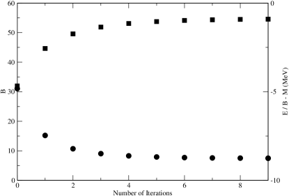
Figure 1: Convergence of the baryon number and binding energy per baryon (boxes and circles respectively) after 9 iterations for an ordinary nucleus of $r_{0}=15/m_{s}$, N = Z, and using the L2 parameter set.

	$g_{s}^{2}$	$g_{v}^{2}$	$m_{s}$	$m_{v}$	$\kappa$	$\lambda$	$g_{s\Lambda}/g_{s}$
L2	109.63	190.43	520	783	0	0	.886601
NLC	95.11	148.93	500.8	783	5000	-200	.881898
Q1	103.67	164.70	504.57	782	4577.6	-197.70	.884029

Table 1: Parameter sets taken from Furnstahl et al. (1997b); Serot and Walecka (1997). $m_{s}$, $m_{v}$, $\kappa$, and $\lambda$ are in MeV. $g_{s\Lambda}/g_{s}$ is fit to reproduce the binding energy of a single $\Lambda$ in nuclear matter Gal et al. (1988).

$g_{s\Xi}/g_{s}$	$\delta\cal{E}/\delta\rho_{B}-\mathrm{M_{\Xi}}$
1	-68.9
.95	-51.6
.9	-34.3

Table 2: Values of the binding energy (in MeV) of a single $\Xi$ in nuclear matter for various $\Xi$ coupling ratios and the parameter set NLC.

III Methodology

In this section we develop a methodology for solving the systems of equations discussed in section 2. In the case of nucleon matter the parameters $g_{s}$, $g_{v}$, $m_{s}$, $m_{v}$, $\mathrm{M}$, $\kappa$, and $\lambda$ must first be specified. The vector meson mass is defined to be the mass of the $\omega$-meson and $\mathrm{M}\equiv 939$ MeV. The remaining constants are given by the three coupling sets in Table 1; to determine these sets the theory was fit to reproduce various properties of ordinary nuclear matter Furnstahl et al. (1997b); Serot and Walecka (1997). The simplest set, L2, includes only linear terms in the scalar field. The sets NLC and Q1 both expand the theory to include nonlinear terms. As a result, these sets must be fit to more properties of nuclear matter than L2.

To extend the theory to systems of nucleons and hyperons, specification of the constants $g_{s\Lambda}$, $g_{s\Xi}$, $g_{v\Lambda}$, and $g_{v\Xi}$ is also required. Since the vector meson is coupled to the conserved baryon current, we assume a universal vector coupling, $g_{v}=g_{v\Lambda}=g_{v\Xi}$. The scalar couplings, on the other hand, are adjusted to reproduce the binding energies of single hyperons in nuclear matter. For instance, the $\Lambda$ scalar coupling is designed to reproduce the binding energy of a single $\Lambda$ in nuclear matter, experimentally determined to be $-28$ MeV Gal et al. (1988). The values of $g_{s\Lambda}/g_{s}$ are also shown in Table 1. Unfortunately data on the binding energy of a single $\Xi$ in nuclear matter is uncertain. Therefore, a range of $\Xi$ scalar couplings is investigated; the values used are $g_{s\Xi}/g_{s}=1$, $.95$, and $.9$. These values correspond to the binding energies listed in Table 2.

Consider the case of infinite nucleon matter. To obtain the solution to this system, first one must specify $k_{F}$. Both Eqs. (14) and (15) are now solved for their respective meson fields. Then, using the meson fields and $k_{F}$, one calculates the energy density in Eq. (13). This is in turn used to evaluate the binding energy per baryon, $\mathrm{BE}(k_{F})\equiv{\cal{E}}/\rho_{B}-\mathrm{M}$. In RMFT the medium saturates and $\mathrm{BE}(k_{F})$ has a minimum; this equilibrium value, $\mathrm{BE_{0}}$, serves as the bulk term in the SEMF, $a_{1}$. This procedure is also applicable to infinite $\Xi N$ and $\Lambda\Xi N$ systems provided the appropriate source terms are included.

Now we discuss the methodology used for all finite systems. First the scalar field Eq. (17) is converted into a pair of coupled first-order finite difference equations for [$\phi_{0}(r)$, $\phi_{0}^{\prime}(r)$]; these equations are solved using a shooting method. To accomplish this, one fixes $\mu$ and $r_{0}$; now the boundary conditions are uniquely determined. Since $k_{F}(r_{0})=0$, we can solve the finite difference equations for $\phi_{0}(r)$ and $\phi_{0}^{\prime}(r)$ one step in. These solutions are substituted back into the constraint equation from which $k_{F}(r)$, one step in, is determined. In this manner we iterate in from the surface, evaluating $\rho_{B}(r)$ and ${\cal{E}}(r)$ at every point. This process is repeated until $\rho_{B}$ and $\phi_{0}$ become constant as $r$ approaches the origin (or equivalently $\rho_{B}^{\prime}=\phi_{0}^{\prime}=0$ at $r=0$); we achieve this by adjusting the chemical potential. We mention that better convergence is obtained by decreasing the step size. Note that initially, $\epsilon$ and $\delta W_{0}$ are ignored.

Now we incorporate the two correction terms. In order to discuss the role of $\epsilon$, let us examine the second boundary condition. When nonlinear terms are introduced, the small parameter, $\epsilon$, is included to compensate. Iterating the finite difference equations out from the surface, $\epsilon$ in Eq. (29) is adjusted such that the scalar field vanishes for large $r$. The newly corrected boundary condition is then used to resolve the finite system by integrating in as described above.

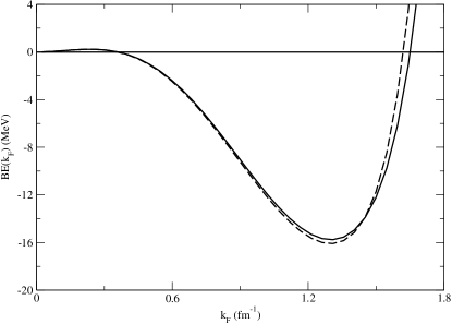
Figure 2: Binding energy per baryon for infinite nuclear matter with N = Z as a function of Fermi wave number. These results are for the coupling sets NLC (solid line) and Q1 (dashed line).

	$k_{F}$	$\mathrm{M^{*}/M}$	$\cal{E}/\rho_{B}-\mathrm{M}$
L2	1.301	.5409	-15.758
NLC	1.301	.6313	-15.768
Q1	1.299	.5975	-16.099

Table 3: Calculated equilibrium values of the Fermi momentum (in $\mathrm{fm^{-1}}$), effective mass, and the $\mathrm{BE_{0}}$ (in MeV) for infinite nucleon matter are shown using the coupling sets in Table 1. These numbers reproduce the results in Furnstahl et al. (1997b); Serot and Walecka (1997).

	$g_{s\Xi}/g_{s}$	$k_{F}$	$\mathrm{M^{*}/M}$	$\cal{E}/\rho_{B}-\mathrm{M_{\Lambda}}$
NLC	1	1.363	.1391	-41.343
	.95	1.351	.1686	-22.747
	.9	1.326	.2232	-4.741
Q1	1	1.320	.1372	-42.728
	.95	1.310	.1643	-24.013
	.9	1.290	.2104	-5.812

Table 4: Calculated equilibrium values of the Fermi momentum (in $\mathrm{fm^{-1}}$), effective mass, and the $\mathrm{BE_{0}}$ (in MeV) for infinite $\Xi N$ matter are shown using the coupling sets NLC and Q1 in Table 1 and a range of values for $g_{s\Xi}/g_{s}$.

Next, the correction term $\delta W_{0}$ is added to the vector field. Initially Eq. (22) was employed; however, this is accurate only in the limit of a large $m_{v}$. A small, but important, contribution to the vector field was omitted; therefore, the term $\delta W_{0}$, defined by Eq. (24) and calculated from the previous $\rho_{B}(r)$, is included. Then the entire process is repeated again. After successive iterations on the vector field, B and $\mathrm{BE}\equiv\mathrm{E}/\mathrm{B}-\mathrm{M}$ both converge to their full solutions. This convergence is illustrated in Fig. 1 for ordinary nucleon matter; here, the parameter set L2 was used, a radius of $r_{0}=15m_{0}^{-1}$ was assumed, and 9 iterations on the vector field have been carried out. Similar convergence was found in all cases studied here.

Finally, we consider the SEMF in Eq. (30) where $a_{1}$ is defined as the $\mathrm{BE}_{0}$ of infinite matter. The calculated values of BE and $\mathrm{B}^{-1/3}$ of the finite systems are plotted against each other for nuclei of various radii. Then using this SEMF as a linear fit, the surface energy, $a_{2}$, is determined. The above approach to finite systems is first calibrated by the nucleon matter case; then it is extended to investigate the $\Xi N$ and $\Lambda\Xi N$ systems detailed in section 2.

IV Results and Discussion

In this section, we discuss the application of the above methodologies. First we consider the results of our infinite matter calculations, starting with nucleon systems. Table 3 shows the equilibrium values of $k_{F}$, $\mathrm{M^{*}/M}$, and $\mathrm{BE_{0}}$ obtained for infinite nucleon matter using the L2, NLC, and Q1 parameter sets. The values calculated here reproduce those in Furnstahl et al. (1997b); Serot and Walecka (1997). Then $\mathrm{BE}(k_{F})$ is plotted for both the NLC and Q1 sets in Fig. 2. The minimum, $\mathrm{BE}_{0}$, in Fig. 2 is taken to be $a_{1}$ in the SEMF for each coupling set. This is in good agreement with the empirical bulk term Walecka (1995).

We now turn our attention to infinite systems of nucleons and hyperons; these investigations are conducted using only the nonlinear cases, NLC and Q1. We begin by investigating infinite $\Xi N$ matter for the range of $\Xi$ scalar couplings mentioned above. Since the lowest mass state of separated baryons under the conditions Eqs. (31) and (32) consists entirely of $\Lambda$’s, $\mathrm{BE}(k_{F})$ for infinite cascade-nucleon matter is defined by $\mathrm{BE}(k_{F})\equiv\cal{E}/\rho_{B}-\mathrm{M_{\Lambda}}$. The calculated equilibrium values for this type of matter are given in Table 4. Notice that $\mathrm{|BE_{0}|}$ decreases as the $\Xi$ coupling grows weaker while the equilibrium $k_{F}$ remains fairly constant. Graphs of $\mathrm{BE}(k_{F})$ for the NLC set and each $\Xi$ scalar coupling ratio shown in Fig. 3 illustrate this point. Although the equilibrium $k_{F}$ is roughly the same here as in the nucleon case, these systems contain twice as many baryons; as a result, the baryon density is much higher than in infinite nucleon matter. Also, the effective mass is considerably smaller, on the order of a third the value of the nucleon case. Again $a_{1}$ in the SEMF for each coupling ratio is taken to be the minimum ($\mathrm{BE_{0}}$) of the corresponding curve in Fig. 3. We also mention that the value of $g_{s\Xi}/g_{s}=.886$ is the lowest $\Xi$ coupling ratio for which infinite $\Xi N$ matter was still bound.

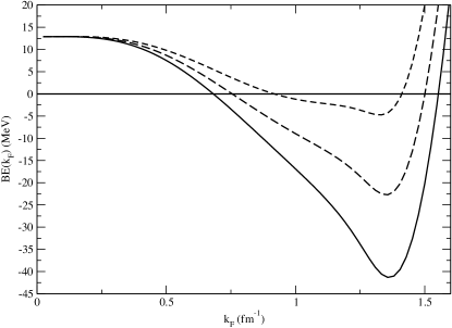
Figure 3: Binding energies per baryon for infinite cascade-nucleon matter computed relative to isolated lambdas (the lowest energy free baryon state for $\mathrm{|S|/B}=1$) as a function of the Fermi wave number using NLC. Note the left hand intercept is $\mathrm{(M_{\Xi}+M_{N})/2-M_{\Lambda}}$. The solid, long dashed, and short dashed lines correspond to $g_{s\Xi}/g_{s}$ = 1, 0.95, and 0.9 respectively.

	$g_{s\Xi}/g_{s}$	$k_{F}$	$k_{F\Lambda}$	$\mathrm{M^{*}/M}$	$\cal{E}/\rho_{B}-\mathrm{M_{\Lambda}}$
NLC	1	1.343	.8665	.1202	-42.229
	.95	1.319	1.026	.1321	-24.704
	.9	1.288	1.159	.1511	-8.100
Q1	1	1.302	.8141	.1213	-43.457
	.95	1.278	.9831	.1325	-25.792
	.9	1.247	1.124	.1495	-9.095

Table 5: Calculated equilibrium values of the Fermi momenta (in $\mathrm{fm^{-1}}$), effective mass, and the $\mathrm{BE_{0}}$ (in MeV) for infinite $\Lambda\Xi N$ matter are shown using the coupling sets NLC and Q1 in Table 1 and a range of values for $g_{s\Xi}/g_{s}$.

Next, we consider infinite $\Lambda\Xi N$ systems using the same range of $\Xi$ scalar couplings quoted above. Note that as in the $\Xi N$ case, $\mathrm{BE}(k_{F})\equiv\cal{E}/\rho_{B}-\mathrm{M_{\Lambda}}$. This investigation produced the equilibrium values shown in Table 5. Here the equilibrium values of $k_{F}$, $\mathrm{M_{*}/M}$, and $\mathrm{BE_{0}}$ differ little from the $\Xi N$ results for large $\Xi$ coupling; however, the difference becomes more pronounced as the $\Xi$ coupling decreases. In our formulation, a second Fermi wave number, $k_{F\Lambda}$, was included for the $\Lambda$’s; as one might expect, $k_{F\Lambda}$ grows, and consequently the proportion of $\Lambda$’s increases, as the gap between $g_{s\Xi}$ and $g_{s\Lambda}$ narrows. The smallest value of the $\Xi$ scalar coupling for which infinite $\Lambda\Xi N$ matter was still bound was $g_{s\Xi}/g_{s}=.875$.

Now we examine the results of the finite matter investigation. To begin with, we consider the finite nucleon matter system. The calculated values of $\mu$, B, $\mathrm{BE=E/B-M}$ as a function of $r_{0}$ for this type of matter using the L2, NLC, and Q1 sets are shown in Table 6. As stated above, 9 iterations on the vector field were conducted on nuclei calculated using the L2 set; this demonstrated the convergence of the system. Subsequent finite nucleon matter results were obtained using 5 iterations which gave results for B and BE to better than $1\%$. The radii used here, $r_{0}=15$, $20$, and $25$ in units of $m_{s}^{-1}$, include nuclei spanning a range of $\mathrm{B}\sim 50-400$. As an example, $\rho_{B}(r)$ and $\phi_{0}(r)$ for a nucleus with $r_{0}=20m_{s}^{-1}$ calculated with the NLC set are displayed in Fig. 4. The interior of the nucleus is roughly constant in both $\rho_{B}(r)$ and $\phi_{0}(r)$. Then the effective mass increases to near unity and the baryon density drops to zero at $r_{0}$; this is a typical example of the surface structure for finite nucleon systems.

Figure 4: The baryon density $n_{B}(r)=\rho_{B}(r)/\mathrm{M^{3}}$ (solid line) and effective mass $\mathrm{M^{*}(r)/M}$ (dashed line) vs. r (in units of $m_{s}^{-1}$) for an ordinary finite nucleus with N = Z, $\mathrm{B}=188.869$ $r_{0}=20/m_{s}$, and using the NLC parameter set.

	$r_{0}$	$\mu$	$\mathrm{B}$	$\mathrm{E/B-M}$
L2	15	4.7055924	54.568	-8.7527
	20	4.69755554	160.72	-10.939
NLC	15	4.6968452	66.438	-11.297
	20	4.69165108	188.87	-12.719
	25	4.68905238	408.43	-13.464
Q1	15	4.6965099	62.581	-11.262
	20	4.69083149	179.76	-12.808
	25	4.68800689	390.77	-13.615

Table 6: Results of finite nucleon matter for the L2, NLC, and Q1 parameter sets and various radii. Calculations with L2 used 9 iterations on the vector field while 5 were used with NLC and Q1. The radii are in $m_{s}^{-1}$, the chemical potential is in $\mathrm{fm^{-1}}$, and $\mathrm{E/B-M}$ is in MeV.

Next using the NLC set the calculated values of BE are plotted vs. $B^{-1/3}$ in Fig. 5 for nuclei of various radii. Notice that the infinite matter value, $\mathrm{BE_{0}}$, has also been included. A SEMF of the form Eq. (30) is used as a linear fit in Fig. 5; the slope of this fit is the surface energy, in this case $a_{2}=18.0$ MeV. The surface energies for the various coupling sets are given in Table 7 along with the experimentally determined value Walecka (1995); the values of $a_{2}$ for both NLC and Q1 show good agreement with experiment. The agreement between the values calculated with the more realistic interactions and the empirical result for the surface energy of ordinary nucleon matter using this effective lagrangian and density functional approach gives us some confidence in our exploratory study of the surface structure of strange superheavy nuclei.

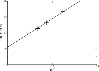
Figure 5: Fit to the calculated SEMF for ordinary nuclear matter with N = Z and the NLC couplings. The surface energy is given by the slope of the curve, here $a_{2}=18.0$ MeV.

	$a_{2}$
L2	26.510
NLC	18.008
Q1	19.107
Expt.	17.8

Table 7: Calculated values of the surface energy (in MeV) for nucleon matter using the parameter sets in Table 1. The experimental value is also included Walecka (1995).

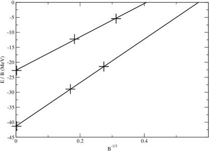
Figure 7: Binding energy vs. $\mathrm{B^{-1/3}}$ for matter composed of equal numbers of cascades and nucleons for the NLC coupling set. The upper and lower curves correspond to $g_{s\Xi}/g_{s}=.95$ and 1 respectively. The surface energy is just the slope of these lines.

Now we investigate finite $\Xi N$ matter for the values of $g_{s\Xi}/g_{s}$ quoted above. Since the best fit to both infinite and finite nucleon matter was obtained with NLC, we use this set exclusively in the following discussion. The values of $\mu$, B, and $\mathrm{BE}=\mathrm{E/B-M_{\Lambda}}$ obtained for finite $\Xi N$ matter are given in Table 8. For the same reasons as in the infinite $\Xi N$ case, the binding energy per baryon is redefined as $\mathrm{BE}\equiv\mathrm{E/B-M_{\Lambda}}$. Note that due to a slower rate of convergence, these systems were calculated using 9 iterations on the vector field. Also the radii, $r_{0}=10$ and $15$ in units of $m_{s}^{-1}$, were used here; this includes nuclei with baryon numbers ranging from $\mathrm{B}\sim 30-200$ depending on the $\Xi$ coupling. It is also important to mention that for the coupling ratio $g_{s\Xi}/g_{s}=.9$, the nuclei were unbound for our choice of radii. For one nucleus of this type, Fig. 6 shows the plots of both $\rho_{B}(r)$ and $\phi_{0}(r)$; this is for a nucleus with $g_{s\Xi}/g_{s}=1$ and $r_{0}=15m_{s}^{-1}$. Notice that the baryon densities in the interior of the nucleus are much larger than those in nucleon matter; also, the effective mass drops to less than a third of the nucleon matter value in the interior. The result is a much higher total B for a fixed $r_{0}$. Another feature of note is the surface structure; here the width of the surface has decreased relative to the previous case. For each of the $\Xi$ scalar coupling ratios, the calculated values of BE are plotted vs. $B^{-1/3}$; these plots are overlaid in Fig. 7. The infinite matter values are also included. As in nucleon matter, the SEMF is used as a linear fit, one for each $\Xi$ coupling ratio, from which the surface energy is determined. The values of $a_{2}$ are given in Table 9.

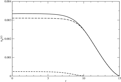
Figure 9: Baryon densities for a finite system of nucleons, cascades, and lambdas with B = 146.248 for the NLC coupling set and $g_{s\Xi}/g_{s}=1$. The total baryon density, the total density of cascades and nucleons, and the lambda density are shown by the solid, long dashed, and short dashed curves respectively. Notice that the lambda density is finite only interior to the surface.

As mentioned in section 2, precise data on the binding energy for a single $\Xi$ in nuclear matter is unavailable. The values appearing in the literature range from -14 to -40 MeV. This necessitated that a number of $\Xi$ scalar couplings be investigated. Now that the surface energies have been acquired for the $\Xi$ couplings, they are plotted vs. these coupling ratios in Fig. 8. A linear interpolation is used between the points; this is extended by extrapolation into the region which corresponds to values of the binding energy of a single $\Xi$ appearing in the literature. We feel confident in the neglect of the $\Lambda$’s over this region because preliminary investigations of finite $\Lambda\Xi N$ matter show that the BE and B change little from $\Xi N$ matter. In Fig. 9 the baryon density of a $\Lambda\Xi N$ nucleus of $r_{0}=10m_{s}^{-1}$ is shown; notice that the $\Lambda$ density begins interior to the surface and is comparatively much smaller.

A preliminary calculation was also conducted with a $\Phi$ meson coupled to the conserved strangeness current. This simulates a repulsion between like strange particles. In order to test the size of this interaction which could be tolerated, the $\Phi$ coupling was increased until the system was no longer bound. The values for which this occurred for infinite $\Xi N$ matter are $g_{\Phi}/g_{\rho}=.68387$, .50902, and .23525 corresponding to $g_{s\Xi}/g_{s}=1$, .95, and .9 respectively.

It should be mentioned that the conditions $\mathrm{Q}=0$ and $\mathrm{|S|/B}=1$ were introduced to eliminate the coulomb and symmetry terms from the SEMF. Since both charge and strangeness are conserved quantities in the strong interaction, these conditions are unaffected by strong (and electromagnetic) reactions in the system. As a result, this is an intrinsically interesting case and the calculation is simplified by the need for only a single Fermi wave number. Of course, experimental processes could produce an arbitrary Q and $\mathrm{|S|/B}$. Therefore it is of interest to estimate how much our results might be modified as these conditions are relaxed.

The SEMF has been generalized to include both nucleons and hyperons in Gal and Dover (1995, 1993); Balberg et al. (1994). The generalized SEMF proposed by Dover and Gal contains additional contributions to the bulk and symmetry energies Gal and Dover (1995). Their SEMF, with their parameter set I, can be used to estimate how much the quantity $\mathrm{E/B}$ changes as one moves away from the conditions $\mathrm{Q}=0$ and $\mathrm{|S|/B}=1$. The additional terms result in $\mathrm{|\delta E/B|}<5$ MeV for the range $1/2<\mathrm{|S|/B}<5/4$ and arbitrary Q. If one makes the rough assumption that the calculated energy could change by this amount, the surface energy extracted from plotting $\mathrm{E/B}$ vs. $\mathrm{B}^{-1/3}$ could change by up to 30% (this is undoubtedly an overestimate). Calculations with arbitrary Q and $\mathrm{|S|/B}$ are more difficult. Work is in progress to examine some of these systems.

It is also of some interest to consider the experimental manifestations of these nuclei. A number of experimental searches for strange matter have been conducted, examples of which are Hill, et al. (2000); Barish, et al. (1997); Armstrong, et al. (2001); Appelquist, et al. (1996); all have yielded negative results. Characteristically, the systems considered here are stable against strong decay but unstable against weak decay. Therefore, their lifetimes are on the order of the weak interaction timescale, or $\sim 10^{-10}$ s. They will experience strangeness changing weak decays, such as the decay modes $\Lambda+\mathrm{N}\rightarrow\mathrm{N+N}$ and $\Xi+\mathrm{N}\rightarrow\mathrm{\Lambda+N}$. We expect heavy ion collisions or supernovae to be possible production sources for these systems. Of course, multistrange baryon systems would have to make transitions to the ground state for the present calculations to be applicable. The actual rate of production of nuclei of the type considered here is a question that goes well beyond the scope of the present paper.

One physical consequence of our results is that the minimum size of these objects is predicted. This value is obtained by setting $\mathrm{E/B}=0$ in the SEMF and then solving for B. The minimum baryon numbers derived from our calculations are 5.4 and 14.6 for $g_{s\Xi}/g_{s}=1$ and .95 respectively. However, shell structure becomes more important in the region of small $\mathrm{E/B}$. As a result, Hartree calculations are more reliable here. Research is in progress to more accurately estimate this number.

In conclusion, we have used this lagrangian density and DFT approach to model nucleon, $\Xi N$, and $\Lambda\Xi N$ matter. First, this approach was used to conduct infinite matter calculations. In the case of infinite nucleon matter, we reproduced the equilibrium values from previous works Furnstahl et al. (1997b); Serot and Walecka (1997). The theory was then extended to infinite $\Xi N$ and $\Lambda\Xi N$ systems; the equilibrium values were also found for these types of matter for various $\Xi$ scalar couplings. The $\mathrm{BE_{0}}$ in each case was taken to be the bulk term in the SEMF. Then we turned our attention to finite systems. For the nucleon matter case, nuclei of various radii were calculated. Plotting BE vs. $\mathrm{B^{-1/3}}$ and using the SEMF as a linear fit, the surface energy was extracted. The values for NLC and Q1 were in good agreement with the experimental value Walecka (1995). This gave us the confidence to extend the finite theory to $\Xi N$ systems. Calculations of $\rho_{B}(r)$ and $\phi_{0}(r)$ gave us a description of the surface structure of these strange superheavy nuclei. Again plotting BE vs. $\mathrm{B^{-1/3}}$ and using the SEMF as a linear fit, the surface energy was extracted for a given $\Xi$ coupling ratio. Then using a linear extrapolation in a plot of $a_{2}$ vs. $g_{s\Xi}/g_{s}$, one can ascertain the surface energy for coupling ratios which correspond to the single $\Xi$ binding energies in the literature.

I would like to thank Dr. J. D. Walecka for his support, advice, and for independently verifying much of the numerical work in this paper. This work was supported in part by DOE grant DE-FG02-97ER41023.

Figure 6: Baryon density $n_{B}(r)=\rho_{B}(r)/\mathrm{M^{3}}$ (solid line) and effective mass $\mathrm{M^{*}(r)/M}$ (dashed line) vs. r (in units of $m_{s}^{-1}$) for a nucleus composed of nucleons and cascades with $r_{0}=15/m_{s}$, $\mathrm{B}=164.918$, and $g_{s\Xi}/g_{s}=1$ subject to the constraints $\mathrm{Q}=0$ and $\mathrm{|S|/B}=1$. These results were obtained using the NLC parameter set.

	$g_{s\Xi}/g_{s}$	$r_{0}$	$\;\;\;\;\>\;\;\;\mu$	$\mathrm{B}$	$\mathrm{E/B-M_{\Lambda}}$
NLC	1	10	1.1604726	48.459	-21.416
		15	1.154255303	204.64	-28.944
	.95	10	1.178092	32.866	-5.4176
		15	1.17206095	164.92	-12.241

Table 8: Results for finite $\Xi N$ matter for the NLC parameter set and a number of radii. These calculations used 9 iterations on the vector field. The radii are in $m_{s}^{-1}$, the chemical potential is in units of $\mathrm{M}$, and $\mathrm{E/B-M_{\Lambda}}$ is in MeV.

Figure 8: Linear fit to the surface energy, $a_{2}$, vs. scalar cascade coupling ratio ($g_{s\Xi}/g_{s}$) for cascade-nucleon matter assuming $\mathrm{Q}=0$, $\mathrm{|S|/B}=1$, and neglecting $\Lambda$’s.

	$g_{s\Xi}/g_{s}$	$a_{2}$
NLC	1	72.687
	.95	55.643

Table 9: Values of the surface energy (in MeV) for $\Xi N$ matter using the NLC parameter set from Table 1.

References

- Schaffner et al. (1993) J. Schaffner, C. Dover, A. Gal, C. Greiner, and H. Stocker, Phys. Rev. Lett. 71, 1328 (1993).
- Schaffner-Bielich and Gal (2000) J. Schaffner-Bielich and A. Gal, Phys. Rev. C62, 034311 (2000).
- Stoks and Lee (1999) V. G. J. Stoks and T. S. H. Lee, Phys. Rev. C60, 024006 (1999).
- Gal et al. (1988) A. Gal, C. Dover, and D. Millener, Phys. Rev. C38, 2700 (1988).
- Gal et al. (1995) A. Gal, E. Friedman, B. K. Jennings, and J. Mares, Nucl. Phys. A594, 311 (1995).
- Dabrowski (1999) J. Dabrowski, Phys. Rev. C60, 025205 (1999).
- Bart, et al. (1999) S. Bart, et al., Phys. Rev. Lett. 83, 5238 (1999).
- Gal (2001) A. Gal, Nucl. Phys. A691, 268c (2001).
- Fukuda, et al. (1998) T. Fukuda, et al., Phys. Rev. C58, 1306 (1998).
- Khaustov, et al. (2000) P. Khaustov, et al., Phys. Rev. C61, 054603 (2000).
- Furnstahl et al. (1996) R. J. Furnstahl, B. Serot, and H.-B. Tang, Nucl. Phys. A598, 539 (1996).
- Walecka (1995) J. D. Walecka, Theoretical Nuclear and Subnuclear Physics (Oxford University Press, 1995).
- Serot and Walecka (1997) B. Serot and J. D. Walecka, Inter. J. of Mod. Phys. E6, 515 (1997).
- Serot and Walecka (1986) B. Serot and J. D. Walecka, Advances in Nuclear Physics, vol. 16 (Plenum Press, 1986).
- Furnstahl et al. (1997a) R. J. Furnstahl, B. Serot, and H.-B. Tang, Nucl. Phys. A618, 446 (1997a).
- Kohn (1999) W. Kohn, Rev. Mod. Phys. 71, 1253 (1999).
- Serot and Walecka (2000) B. Serot and J. D. Walecka, 150 Years of Quantum Many-body Theory (World Scientific, 2000), p. 203.
- Yamamoto et al. (1994) Y. Yamamoto, T. Motoba, H. Himeno, K. Ikeda, and S. Nagata, Prog. Theor. Phys. Suppl. 117, 361 (1994).
- Witten (1984) E. Witten, Phys. Rev. D30, 272 (1984).
- Farhi and Jaffe (1984) E. Farhi and R. L. Jaffe, Phys. Rev. D30, 2379 (1984).
- Mares and Zofka (1993) J. Mares and J. Zofka, Z. Phys. A345, 47 (1993).
- Rufa et al. (1990) M. Rufa, J. Schaffner, J. Maruhn, H. Stocker, W. Greiner, and P. G. Reinhard, Phys. Rev. C42, 2469 (1990).
- Barranco et al. (1991) M. Barranco, R. J. Lombard, S. Marcos, and S. A. Moszkowski, Phys. Rev. C44, 178 (1991).
- Lanskoy and Tretyakova (1992) D. E. Lanskoy and T. Y. Tretyakova, Z. Phys. A343, 355 (1992).
- Schulze et al. (1998) H. J. Schulze, M. Baldo, U. Lombardo, J. Cugnon, and A. Lejeune, Phys. Rev. C57, 704 (1998).
- Gal and Dover (1995) A. Gal and C. Dover, Nucl. Phys. A585, 1c (1995).
- Schaffner et al. (1994) J. Schaffner, C. Dover, A. Gal, C. Greiner, J. Millener, and H. Stocker, Ann. of Phys. 235, 35 (1994).
- Gal and Dover (1993) A. Gal and C. Dover, Nucl. Phys. A560, 559 (1993).
- Balberg et al. (1994) S. Balberg, A. Gal, and J. Schaffner, Prog. Theor. Phys. Suppl. 117, 325 (1994).
- Stoks et al. (1999) V. G. J. Stoks, T. A. Rijken, and Y. Yamamoto, Phys. Rev. C59, 21 (1999).
- Stoks and Rijken (1999) V. G. J. Stoks and T. A. Rijken, Phys. Rev. C59, 3009 (1999).
- Halderson (1999) D. Halderson, Phys. Rev. C60, 064001 (1999).
- Rijken (1998) T. A. Rijken, Nucl. Phys. A639, 29c (1998).
- Vidana et al. (2000) I. Vidana, A. Polls, A. Ramos, H. Hjorth-Jensen, and V. G. J. Stoks, Phys. Rev. C61, 025802 (2000).
- Wang et al. (1999) P. Wang, R. K. Su, H. Q. Song, and L. L. Zhang, Nucl. Phys. A653, 166 (1999).
- Balberg and Gal (1997) S. Balberg and A. Gal, Nucl. Phys. A625, 435 (1997).
- Banik and Bandyopadhyay (2000) S. Banik and D. Bandyopadhyay, J. Phys. G26, 1495 (2000).
- Baldo et al. (2000) M. Baldo, G. F. Burgio, and H. J. Schultze, Phys. Rev. C61, 055801 (2000).
- Glendenning (1997) N. Glendenning, Compact Stars: Nuclear Physics, Particle Physics, and General Relativity (Springer, 1997).
- Furnstahl et al. (1997b) R. J. Furnstahl, B. Serot, and H.-B. Tang, Nucl. Phys. A615, 441 (1997b).
- Hill, et al. (2000) J. C. Hill, et al., Nucl. Phys. A675, 226c (2000).
- Barish, et al. (1997) K. N. Barish, et al., Jour. Phys. G23, 2127 (1997).
- Armstrong, et al. (2001) T. A. Armstrong, et al., Phys. Rev. C63, 054903 (2001).
- Appelquist, et al. (1996) G. Appelquist, et al., Phys. Rev. Lett. 76, 3907 (1996).