Vector meson production and nucleon resonance analysis in a coupled-channel approach for energies $m_{N}<\sqrt{s}<2$ GeV
II: photon-induced results

Abstract

We present a nucleon resonance analysis by simultaneously considering all pion- and photon-induced experimental data on the final states $\gamma N$, $\pi N$, $2\pi N$, $\eta N$, $K\Lambda$, $K\Sigma$, and $\omega N$ for energies from the nucleon mass up to $\sqrt{s}=2$ GeV. In this analysis we find strong evidence for the resonances $P_{31}(1750)$, $P_{13}(1900)$, $P_{33}(1920)$, and $D_{13}(1950)$. The $\omega N$ production mechanism is dominated by large $P_{11}(1710)$ and $P_{13}(1900)$ contributions. In this second part we present the results on the photoproduction reactions and the electromagnetic properties of the resonances. The inclusion of all important final states up to $\sqrt{s}=2$ GeV allows for estimates on the importance of the individual states for the GDH sum rule.

I Introduction

The reliable extraction of nucleon resonance properties from experiments where the nucleon is excited via either hadronic or electromagnetic probes is one of the major issues of hadron physics. The goal is to be finally able to compare the extracted masses and partial-decay widths to predictions from lattice QCD (e.g., Ref. flee ) and/or quark models (e.g., Refs. capstick ; riska ).

With this aim in mind, in Refs. feusti98 ; feusti99 we developed a unitary coupled-channel effective Lagrangian model that incorporated the final states $\gamma N$, $\pi N$, $2\pi N$, $\eta N$, and $K\Lambda$, and was used for a simultaneous analysis of all avaible experimental data on photon- and pion-induced reactions on the nucleon. The premise is to use the same Lagrangians for the pion- and photon-induced reactions, allowing for a consistent analysis, thereby generating the background dynamically from $u$ and $t$ channel contributions without new parameters. In the preceding paper pm1 , called PMI in the following, we presented the results of the extension of the model space to center-of-mass energies of $\sqrt{s}=2$ GeV, which requires the additional incorporation of the final states $\omega N$ and $K\Sigma$. The ingredients mandatory for a unitary description of all the above final states and the results on the pion-induced reactions have been discussed both for calculations where only the pion-induced reactions were considered and calculations where pion- and photon-induced reactions were considered. In this paper, we concentrate on the photoproduction reactions.

For the photoproduction of the newly incorporated channels $\omega N$ and $K\Sigma$, almost all models in the literature are based on single-channel effective Lagrangian calculations ignoring rescattering effects (often called “$T$-matrix models”). Especially the inclusion of nucleon Born contributions for the $\omega$ production mechanism in these models has led to an overestimation of the data for energies above $\sim 1.77$ GeV, and only either the neglect of these diagrams or very soft form factors has resulted in a rough description of the experimental data. In the first calculation on $\omega$ photoproduction, performed by Friman and Soyeur frimansoyeur , a rough description of the experimental data was achieved by only including $\pi$ and $\sigma$ $t$-channel exchange. In the model of Oh and co-workers oh ; oh01 the nucleon contributions are damped by rather soft form factors [$\Lambda_{N}=0.5-0.7$ GeV using $F_{p}$, Eq. (13)]. A similar observation was made in the model of Babacan et al. babacan , where the Born contributions were not damped by soft form factors, but a very small $\omega NN$ coupling constant was extracted ($g_{\omega NN}\leq 1$). Hence in both models, the Born contributions are effectively neglected. Since Babacan et al. did not include any baryon resonances, the effective reaction process is almost purely given by $t$-channel exchanges, and is thus close to the model of Friman and Soyeur. Oh et al., however, included baryon resonances by using nonrelativistic Breit-Wigner descriptions with vertex functions taken from the quark model of Capstick capstick and thus did not consistently generate a $u$-channel background. An imaginary part of the amplitude was only taken into account via total widths in the denominator of the implemented Breit-Wigner resonance description. In a similar way resonances were also included in the effective Lagrangian quark model of Zhao and co-workers zhao ; zhao01 ; zhao02 on $\omega$ photoproduction. However, none of these models on $\omega$ photoproduction included rescattering effects. Only in the most recent two works of Oh and co-workers oh did the authors start to consider the coupled-channel effects of intermediate $\pi N$ and $\rho N$ states.

This restriction to a single-channel analysis is a fundamental weakness of all the $T$-matrix models. Although the above models on $\omega N$ and also single-channel analyses on $K\Lambda$ or $K\Sigma$ adelseck ; martbenn ; mart ; lee01 ; cheoun photoproduction aim to provide a tool for the search and identification of missing resonances, an inherent problem of such an extraction is ignored: Due to the restriction on one single reaction channel, rescattering effects can only be incorporated in those models by putting in by hand a total width in the denominator of the included resonances. It often cannot be examined whether the applied resonance parameters are compatible with other reaction channels. Thus the “hunt for hidden resonances” by single channel analyses becomes questionable.

This problem can only be circumvented if all channels are compared simultaneously to experimental data, thereby restricting the freedom severely; this is done in the model underlying the present calculation. The aim of this paper is to discuss the results of the photoproduction reactions. We start in Sec. II with a review of the necessary extension of the model for the inclusion of photoproduction reactions. In Sec. III the implemented data base is discussed and the changes with respect to Ref. feusti99 are pointed out. In Sec. IV our calculations are compared to the available experimental data, and we conclude with a summary. In the Appendices, we give a summary of the extensions of the formalism underlying the present calculations necessary for the inclusion of photoproduction reactions; more details can be found in PMI pm1 and Ref. gregiphd .

II Inclusion of Photoproduction in the Giessen Model

For the inclusion of photon-induced reactions in the Bethe-Salpeter equation (see Appendix B and PMI pm1 ),

$${\mathcal{T}}^{fi}_{\lambda^{\prime}\lambda}={\mathcal{K}}^{fi}_{\lambda^{\prime}\lambda}+\mbox{i}\int\mathrm{d}\Omega_{a}\sum_{a}\sum_{\lambda_{a}}{\mathcal{T}}^{fa}_{\lambda^{\prime}\lambda_{a}}{\mathcal{K}}^{ai}_{\lambda_{a}\lambda}\;,$$ (1)

a full isospin decomposition of the photon-induced reactions including Compton scattering has to be performed. In Eq. (1), $a$ represents the intermediate two-particle state. Although this decomposition can in principle be easily achieved (see Ref. gregiphd ), one runs into problems concerning gauge invariance of Compton scattering. This is due to the fact that the rescattering takes place via the $I=\frac{1}{2}$ and $\frac{3}{2}$ amplitudes, thus weighing the Compton isospin amplitudes $T^{11,\frac{1}{2}}_{\gamma\gamma}$ with $I=\frac{1}{2}$ and $T^{11,\frac{3}{2}}_{\gamma\gamma}$ with $I=\frac{3}{2}$ of Eq. (56) differently, while gauge invariance for the nucleon contributions is only fulfilled for the proton and neutron amplitude (more precisely, for the combination $T^{11,\frac{1}{2}}_{\gamma\gamma}+2T^{11,\frac{3}{2}}_{\gamma\gamma}$). This is related to the fact that only two physical amplitudes for Compton scattering exist ($\gamma p\rightarrow\gamma p$, $\gamma n\rightarrow\gamma n$) and rescattering effects are usually calculated in a basis using physical ($\pi^{0}p$, $\pi^{+}n$, $\pi^{-}p$, $\pi^{0}n$), not isospin states ben92 . Consequently, the electromagnetic interaction is included only perturbatively in the present calculation model. The perturbative inclusion is equivalent to neglecting all intermediate electromagnetic states $a$ in the rescattering part of Eq. (1). Due to the smallness of the fine structure constant $\alpha$, this approximation is reasonable. The consequence is that the calculation of the hadronic reactions decouples from the electromagnetic ones and can be extracted independently. Hence the full partial-wave decomposed $K$-matrix equation

$${\mathcal{T}}^{IJ\pm}_{fi}=\left[\frac{{\mathcal{K}}^{IJ\pm}}{1-\mbox{i}{\mathcal{K}}^{IJ\pm}}\right]_{fi}\;,$$ (2)

where ${\mathcal{K}}\propto\langle f|K|i\rangle=\langle f|V|i\rangle$ [see Eq. (39) in Appendix B], is only solved for the hadronic states. In the second step, the meson photoproduction amplitudes can be extracted via

$${\mathcal{T}}^{IJ\pm}_{f\gamma}={\mathcal{K}}^{IJ\pm}_{f\gamma}+\mbox{i}\sum\limits_{a}{\mathcal{T}}^{IJ\pm}_{fa}{\mathcal{K}}^{IJ\pm}_{a\gamma}\;,$$ (3)

where the helicity indices are omitted. The sum runs only over hadronic states. Finally, the Compton amplitudes result from

$${\mathcal{T}}^{IJ\pm}_{\gamma\gamma}={\mathcal{K}}^{IJ\pm}_{\gamma\gamma}+\mbox{i}\sum\limits_{a}{\mathcal{T}}^{IJ\pm}_{\gamma a}{\mathcal{K}}^{IJ\pm}_{a\gamma}$$ (4)

with $a$ running again only over hadronic states. Since the Compton isospin amplitudes of the potential only enter in the direct contribution ${\mathcal{K}}^{IJ\pm}_{\gamma\gamma}$ and only the proton and neutron Compton amplitudes of Eq. (57) are of interest, gauge invariance is fulfilled.

II.1 Electromagnetic part of the potential

The contributions to the potential $V$ in the case of photon-induced reactions come from bremsstrahlung of asymptotic particles ($N$, $\Sigma$, $\pi$, $K$), electromagnetic decays of nucleon resonances, and intermediate (vector) mesons. Since the corresponding Lagrangians have already been given in Ref. feusti99 , we only present a short summary of the electromagnetic part of the interaction, which is added to the hadronic part specified in PMI pm1 . The $s$-, $u$-, and $t$-channel Born contributions and the Kroll-Rudermann term are generated by

$${\mathcal{L}} = -e\bar{u}_{B^{\prime}}(p^{\prime})\left[\left(\hat{e}\gamma_{\mu}A^{\mu}+\frac{\kappa}{2m_{N}}\sigma_{\mu\nu}F^{\mu\nu}\right)+\frac{g_{\varphi}}{m_{B}+m_{B^{\prime}}}\gamma_{5}\gamma_{\mu}A^{\mu}\right]u_{B}(p)$$ (5)

$$-\mbox{i}\hat{e}e\varphi^{*}\left(\partial_{\mu}^{\varphi}-\partial_{\mu}^{(\varphi^{*})}\right)\varphi A^{\mu}-e\frac{g_{\varphi}}{m_{B}+m_{B^{\prime}}}\bar{u}_{B^{\prime}}(p^{\prime})\gamma_{5}\gamma_{\mu}u_{B}(p)A^{\mu}$$

with the asymptotic baryons $B,B^{\prime}=(N,\Lambda,\Sigma)$, the pseudoscalar mesons $(\varphi,\varphi^{\prime})=(\pi,K)$ and $F^{\mu\nu}=\partial^{\mu}A^{\nu}-\partial^{\nu}A^{\mu}$.

For the intermediate ($t$-channel) mesons, which are summarized in Table 1,

	mass [GeV]	$S$	$P$	$I$	$t$-channel contributions
$\pi$	0.138	$0$	$-$	$1$	$(\gamma,\gamma),(\gamma,\pi),(\gamma,\omega)$
$K$	0.496	$0$	$-$	$\frac{1}{2}$	$(\gamma,\Lambda),(\gamma,\Sigma)$
$\eta$	0.547	$0$	$-$	$0$	$(\gamma,\gamma),(\gamma,\omega)$
$\omega$	0.783	$1$	$-$	$0$	$(\gamma,\pi),(\gamma,\eta)$
$\rho$	0.769	$1$	$-$	$1$	$(\pi,\pi),(\pi,\omega),(\gamma,\pi),(\gamma,\eta)$
$K^{*}$	0.894	$1$	$-$	$\frac{1}{2}$	$(\pi,\Lambda),(\pi,\Sigma),(\gamma,\Lambda),(\gamma,\Sigma)$
$K_{1}$	1.273	$1$	$+$	$\frac{1}{2}$	$(\gamma,\Lambda),(\gamma,\Sigma)$

Table 1: Properties of asymptotic and intermediate $t$-channel mesons entering the potential for the photon-induced reactions. For those particles, that appear in several charge states, averaged masses are used. In the last column, all reaction channels (including pion- induced), to which the mesons contribute, are given.

the additional Lagrangian

$${\mathcal{L}}=-\mbox{i}g_{K_{1}}\left(\gamma_{\mu}K_{1}^{\mu}+\frac{\kappa_{K_{1}}}{2m_{N}}\sigma_{\mu\nu}K_{1}^{\mu\nu}\right)\gamma_{5}u_{B}(p)-\frac{g}{4m_{\varphi}}\varepsilon_{\mu\nu\rho\sigma}V^{\mu\nu}{V^{\prime}}^{\rho\sigma}\varphi+e\frac{g_{K_{1}K\gamma}}{2m_{K}}KF_{\mu\nu}K_{1}^{\mu\nu}$$ (6)

is taken. $V^{\mu\nu}$ and $K_{1}^{\mu\nu}$ are defined in analogy to $F^{\mu\nu}$. Note that the second term in Eq. (6) summarizes all processes as, e.g., $\omega\rightarrow\gamma\pi$ and $\pi/\eta\rightarrow\gamma\gamma$. The meson and baryon coupling constants entering Eqs. (5) and (6) are summarized in Appendix A.

The radiative decay of the spin-$\frac{1}{2}$ resonances is described by

$${\mathcal{L}}_{\frac{1}{2}N\gamma}=-e\frac{g_{1}}{4m_{N}}\bar{u}_{R}\left(\begin{array}[]{c}1\\ -\mbox{i}\gamma_{5}\end{array}\right)\sigma_{\mu\nu}u_{N}F^{\mu\nu}$$ (9)

and for the spin-$\frac{3}{2}$ resonances by

$${\mathcal{L}}_{\frac{3}{2}N\gamma}=\bar{u}_{R}^{\mu}e\left(\begin{array}[]{c}\mbox{i}\gamma_{5}\\ 1\end{array}\right)\left(\frac{g_{1}}{2m_{N}}\gamma^{\nu}+\mbox{i}\frac{g_{2}}{4m_{N}^{2}}\partial^{\nu}_{N}\right)u_{N}F_{\mu\nu}\;.$$ (12)

In Eqs. (9) and (12), the upper (lower) factor corresponds to positive- (negative-) parity resonances. Note that in the spin-$\frac{3}{2}$ case, both couplings are in addition contracted by an off-shell projector $\Theta_{\mu\nu}(a)=g_{\mu\nu}-a\gamma_{\mu}\gamma_{\nu}$, where $a$ is related to the commonly used off-shell parameter $z$ by $a=(z+\mbox{$\frac{1}{2}$})$ (see PMI pm1 for more details).

The calculation of the amplitudes, the extraction of electromagnetic multipoles from partial waves, the isospin decomposition, and the calculation of observables are given in Appendices A, B, C, D, and E, respectively.

II.2 Form factors and gauge invariance

To account for the internal structure of the mesons and baryons, as in Refs. feusti98 ; feusti99 , the following form factors are introduced at the vertices:

$$F_{p}(q^{2},m^{2}) = \frac{\Lambda^{4}}{\Lambda^{4}+(q^{2}-m^{2})^{2}}\;,$$ (13)

$$F_{t}(q^{2},m^{2}) = \frac{\Lambda^{4}+\frac{1}{4}(q_{t}^{2}-m^{2})^{2}}{\Lambda^{4}+\left(q^{2}-\frac{1}{2}(q_{t}^{2}+m^{2})\right)^{2}}\;.$$ (14)

Here $q_{t}^{2}$ denotes the value of $q^{2}$ at the kinematical threshold of the corresponding $s$, $u$, or $t$ channel. As in Ref. feusti98 , the form factor $F_{p}$ is applied to all $s$- and $u$-channel baryon resonance vertices and to all hadronic $s$- and $u$-channel Born vertices. Only in the $t$-channel diagrams have calculations been performed using either $F_{p}$ or $F_{t}$ at the meson-baryon-baryon vertex, see Sec. IV.

In an effective Lagrangian model, the question of gauge invariance can be addressed on a fundamental level. Since the above resonance and intermediate meson electromagnetic decay vertices fulfill gauge invariance by construction ($\Gamma_{\mu}k^{\mu}=0$, where $k_{\mu}$ is the photon momentum), these vertices and the corresponding hadronic vertices can be independently multiplied by form factors. However, it is well known that the inclusion of hadronic form factors in the Born diagrams of photoproduction reactions leads to problems, because only the sum of all charge contributions of the Born diagrams contributing to one specific reaction is gauge invariant. Form factors at the hadronic vertices of these diagrams lead to putting $q^{2}$-dependent weights on the different diagrams; thus the sum becomes misbalanced and gauge invariance is violated. In order to restore gauge invariance, one needs to construct additional current contributions beyond the usual Feynman diagrams (contact diagrams) to cancel the gauge violating terms. As pointed out by Haberzettl haberzettl (see also the detailed discussion in Ref. feusti99 ) the effect of the additional current contributions is to replace the hadronic form factors multiplying the charge contributions of the Born diagrams in pion photoproduction by a common form factor $\hat{F}(s,u,t)$. In the present model we follow Davidson and Workman davidson01 , who proposed a crossing symmetric shape for this form factor $\hat{F}(s,u,t)$, which ensures that the additional current contributions are pole-free:

$$\hat{F}(s,u,t)=F_{1}(s)+F_{2}(u)+F_{3}(t)-F_{1}(s)F_{2}(u)-F_{1}(s)F_{3}(t)-F_{2}(u)F_{3}(t)+F_{1}(s)F_{2}(u)F_{3}(t)\;.$$ (15)

This form can also be applied easily to $\eta$ and $\omega$ photoproduction by setting $F_{3}(t)=0$ and to $K\Lambda$ photoproduction by setting $F_{2}(u)=0$, since the corresponding Born diagrams are absent. Furthermore, no form factors are used at the electromagnetic vertices of the Born diagrams, see Refs. feusti99 and gregiphd . Note that Feuster and Mosel feusti99 used the Haberzettl suggestion for the common form factor multiplying the charge contributions of the Born diagrams,

$$\hat{F}(s,u,t)=a_{1}F_{1}(s)+a_{2}F_{2}(u)+a_{3}F_{3}(t)\;.$$ (16)

with $a_{1}=a_{2}=a_{3}=\frac{1}{3}$.

III Experimental Data Base

In this section, the implemented experimental photoproduction data base is presented, especially in view of changes and extensions as compared to Ref. feusti99 . A summary of all references and more details on data base weighing and error treatment are given in Ref. gregiphd .

$\mathbf{\gamma N\rightarrow\pi N}$:
For pion photoproduction we have implemented the continuously updated single-energy multipole analysis of the Virginia Polytechnic Institute (VPI) group SP01 , which greatly simplifies the analysis of experimental data within the coupled-channel formalism. For those energies, where the single-energy solutions have not been available, the gaps have been filled with the energy-dependent solution of the VPI group. Since the latter data are model dependent, they enter the fitting procedure only with enlarged error bars.

$\mathbf{\gamma N\rightarrow 2\pi N}$:
As discussed in PMI pm1 , for simplicity we continue to parametrize the $2\pi N$ final state by an effective $\zeta N$ state, where the $\zeta$ is an isovector scalar meson with mass $m_{\zeta}=2m_{\pi}$. A consequence is that the $\zeta N$ state is only allowed to couple to baryon resonances, since only in this case the decay of the resonance into $\zeta N$ can be interpreted as the total ($\sigma N+\pi\Delta+\rho N+\dots$) $2\pi N$ width. As it turns out in the pion-induced calculations, a qualitative description of the $\pi N\rightarrow 2\pi N$ partial waves extracted by Manley et al. manley84 up to $J=\frac{3}{2}$ is possible. The same agreement as in the pion-induced $2\pi N$ production, however, cannot be expected in the $2\pi N$ photoproduction reaction. It has been shown (e.g., Refs. hirata ; murphy ; oset ) that the $\gamma N\rightarrow 2\pi N$ reactions require strong background contributions from, e.g, $\rho$ contact interactions, which can only be included in the present model by the introduction of separate $2\pi N$ final states. Furthermore, there is no partial-wave decomposition of this reaction as the one by Manley et al. for $\pi N\rightarrow 2\pi N$ manley84 , which is the only way for comparing our $\zeta N$ production with experiment. Therefore, the $\gamma N\rightarrow 2\pi N$ reaction is calculated in the model and included in the rescattering summation, but not compared to experimental data; see also Sec. IV.7.

$\mathbf{\gamma N\rightarrow\gamma N}$:
In addition to the data used in Ref. feusti99 , the differential cross sections and beam-polarization data of Ref. datagg are implemented. Since the spin-$\frac{5}{2}$ resonances $D_{15}(1675)$ and $F_{15}(1680)$ are known to have large photon couplings pdg , it is certain, that for higher energies their contributions will be important. Therefore, we continue to compare Compton scattering only up to a maximum energy of $1.6$ GeV.

$\mathbf{\gamma N\rightarrow\eta N}$:
We have added the differential and total cross sections, beam- and target polarizations from Ref. datage . All of the published cross section data concentrate almost exclusively on the energy region below $1.7$ GeV. Only recently, the CLAS collaboration dugger also accessed the energy region above $1.7$ GeV. Therefore, the preliminary CLAS data, more than 100 data points of which are directly included in the fitting procedure, are also important to obtain a handle on the higher energy region of $\eta$ photoproduction and are consequently included.

$\mathbf{\gamma N\rightarrow K\Lambda}$:
The recent cross section and $\Lambda$ polarization measurements of the SAPHIR Collaboration datagl have been added.

$\mathbf{\gamma N\rightarrow K\Sigma}$:
For this reaction, experimental data on cross sections and the $\Sigma$ polarization for $\gamma p\rightarrow K^{+}\Sigma^{0}/K^{0}\Sigma^{+}$ are included datags .

$\mathbf{\gamma N\rightarrow\omega N}$:
For this reaction, only the cross section measurements of the ABBHHM Collaboration erbeom and of Crouch et al. crouch are published up to now. Using only these data, even in combination with the pion-induced data, it is difficult to extract the $\omega N$ couplings reliably. Thus, in addition we have also considered the very precise preliminary differential cross section data of the SAPHIR Collaboration barthom , more than 140 data points of which are directly included in the fitting procedure.

Altogether, more than 4400 photoproduction (plus 2400 pion-induced) data points are included in the fitting strategy, which are binned into $96$ energy intervals; for each angle differential observable we allow for up to $10-15$ data points per energy bin.

IV Results on Photon-Induced Reactions

The details of the calculations to extract the resonance couplings and masses by comparison with experimental data are discussed in PMI pm1 . Here we only shortly review the properties of the global calculations, where the photoproduction data are also considered for the determination of the parameters. For these calculations, we have extended the four best hadronic fits C-p-$\pi\pm$ and C-t-$\pi\pm$. Here the first letter C denotes that the conventional spin-$\frac{3}{2}$ couplings with spin-$\frac{1}{2}$ off-shell contributions are used (see PMI pm1 ), the next letter “p” or “t” denotes whether the form factor $F_{p}$ [Eq. (13)] or $F_{t}$ [Eq. (14)] is used in the $t$-channel diagrams, $\pi$ stands for using only pion-induced data, and the last letter denotes the a priori unknown sign of the coupling $g_{\omega\rho\pi}$. Note that this coupling gives rise to the important $t$-channel $\rho$ exchange in $\pi N\rightarrow\omega N$. Correspondingly, the four global calculations are labeled C-p-$\gamma\pm$ and C-t-$\gamma\pm$.

Similar to Feuster and Mosel feusti99 , our first attempt for the inclusion of the photoproduction data in the calculation has been to keep all hadronic parameters fixed to their values obtained in the fit to the pion-induced reactions. In contrast to the findings of Ref. feusti99 , no satisfactory description of the photoproduction reactions has been achieved with these hadronic parameters. As a consequence of the smaller data base used in Ref. feusti99 at most three photoproduction reactions ($\gamma N\rightarrow\gamma N$, $\gamma N\rightarrow\pi N$, $\gamma N\rightarrow\eta N$) had to be fitted simultaneously. Above 1.6 GeV, no data were available on $\eta$ photoproduction.

The extended model space and data base now constrains all production mechanisms more strongly, especially for energies above 1.7 GeV, where precise photoproduction data on all reactions (besides Compton scattering) are used. Due to the lack of precise data in the high energy region for pion-induced $\eta N$ and $\omega N$ production, these production mechanisms have not been correctly decomposed in the purely hadronic calculations, thus leading to contradictions in the photoproduction reactions when the hadronic parameters are kept fixed. Moreover, as pointed out in PMI pm1 , the Born couplings in the associated strangeness production only play a minor role in the pion-induced reactions while, as a result of the gauging procedure, these contributions are enhanced in photoproduction thus allowing for a more reliable determination of the corresponding couplings. Consequently, the $K\Lambda/\Sigma$ photoproduction also turns out to be hardly describable when the hadronic parameters are kept fixed. Only when also these parameters are allowed to vary a simultaneous description of all pion- and photon-induced reactions is possible.

The resulting $\chi^{2}$ values for the calculations C-p-$\gamma\pm$ are presented in Table 2;

Fit	Total $\pi$	$\chi^{2}_{\pi\pi}$	$\chi^{2}_{\pi 2\pi}$	$\chi^{2}_{\pi\eta}$	$\chi^{2}_{\pi\Lambda}$	$\chi^{2}_{\pi\Sigma}$	$\chi^{2}_{\pi\omega}$
C-p-$\gamma+$	3.78	4.23	7.58	3.08	3.62	2.97	1.55
C-p-$\gamma-$	4.17	4.09	8.52	3.04	3.87	3.94	3.73
SM95-pt-3	6.09	5.26	18.35	2.96	4.33	—	—
Fit	Totala	$\chi^{2}_{\gamma\gamma}$	$\chi^{2}_{\gamma\pi}$	$\chi^{2}_{\gamma\eta}$	$\chi^{2}_{\gamma\Lambda}$	$\chi^{2}_{\gamma\Sigma}$	$\chi^{2}_{\gamma\omega}$
C-p-$\gamma+$	6.57	5.30	10.50	2.45	3.95	2.74	6.25
C-p-$\gamma-$	6.66	5.15	10.54	2.37	2.85	2.27	6.40
SM95-pt-3	24.40	16.45	42.07	8.01	4.64	—	—

Table 2: Resulting $\chi^{2}$ of the various fits. For comparison, we have also applied the preferred parameter set SM95-pt-3 of Ref. feusti99 to our extended and modified data base for energies up to $1.9$ GeV. ^a: This value includes all pion- and photon-induced data points.

for the results of the calculations C-t-$\gamma\pm$ see below. Note that, in contrast to the previous analysis feusti99 , in the present calculation we have included all experimental data up to the upper end of the energy range, in particular also for all partial- wave and multipole data up to $J=\frac{3}{2}$. At first sight it seems that the total $\chi^{2}$ is only fair; however, one has to note that the main part of this value stems from the pion-photoproduction multipoles SP01 , which have very small error bars but also scatter a lot (cf. Figs. 3 – 5 in Sec. IV.2 below). Note, that in this channel, there are 40% of all data points. Taking this channel out, the total $\chi^{2}$ per data point is reduced from $6.56$ to $3.87$ for the preferred global fit. Thus a very good simultaneous description of all reactions is possible, which shows that the measured data for all reactions are compatible with each other, concerning the partial-wave decomposition and unitarity effects. As a guideline for the quality of the present calculation, we have also included a comparison with the preferred parameter set SM95-pt-3 of Ref. feusti99 applied to our extended and modified data base. It is interesting to note that although this comparison has only taken into account data up to 1.9 GeV for the final states $\gamma N$, $\pi N$, $2\pi N$, $\eta N$, and $K\Lambda$, the present best global calculation C-p-$\gamma+$ results in a better description in almost all channels; only for $\pi N\rightarrow\eta N$ the $\chi^{2}$ of Ref. feusti99 is slightly better. This is a consequence of the fact that, for example, for the understanding of $K\Lambda$ production, the coupled-channel effects due to the final states $K\Sigma$ and $\omega N$ have to be included. This is discussed in Sec. IV.4 below.

Moreover, while in Ref. feusti98 similar results were found using either one of the form factors $F_{t}$ and $F_{p}$ for the $t$-channel meson exchanges, and in Ref. feusti99 only $F_{t}$ was applied, the extended data base and model space shows a clear preference of using the form factor $F_{p}$ for all vertices, i.e., also for the $t$-channel meson exchange. We have also tried to perform global fitting calculations using $F_{t}$ in the $t$-channel exchange processes (C-t-$\gamma\pm$), but have not found any satisfactory parameter set for a global description in this case. Even when the fitting procedure has been reduced to the five most important final states — $\gamma N$, $\pi N$, $2\pi N$, $\eta N$, and $\omega N$ — we have found for $\gamma/\pi N\rightarrow\eta N$ $\chi^{2}$’s of only $\approx 5$ and for $\gamma N\rightarrow\omega N$ ($\pi N\rightarrow\omega N$) $\chi^{2}$’s of $\approx 30$ ($\approx 7$), while pion production and Compton scattering have been only slightly worse as compared to C-p-$\gamma\pm$. The much worse description using $F_{t}$ in the global fits can be explained by the fact that, for the photon-induced reactions, the $NN\omega$ coupling now not only appears as a final state coupling, but also contributes in the production of $\pi N$ and $\eta N$. Conversely the $\pi NN$ coupling constant is now also of great importance in $\omega$ photoproduction. Thereby, the validity of the form factors is tested in a wide kinematical region, since, in our model, many of the $t$-channel meson couplings contribute to several reactions and also as final state couplings (cf. Table 1 above). We conclude that $F_{p}$ is applicable to a much wider kinematic region (especially to higher energies) than $F_{t}$. This comes about because of the quite different $q^{2}$-dependent behavior of the two form factors $F_{p}$ and $F_{t}$ below the pole mass and in the low $|t|=|q^{2}|$ region. To find satisfactory results with the form factor $F_{t}$ in the present model, it would be necessary to lift the restriction of using only one cutoff value $\Lambda_{t}$ for all $t$-channel diagrams.

In the following sections, the photoproduction results of the two global calculations C-p-$\gamma+$ and C-p-$\gamma-$ are discussed in detail.

IV.1 Compton scattering

A simultaneous description of Compton scattering together with the inelastic channels is essential because this process is dominated by the electromagnetic coupling and may thus impose more stringent requirements on those. As a consequence of the new data from Ref. datagg we have doubled the Compton scattering data base from 266 to 538 data points as compared to Ref. feusti99 . This means that the description of Compton scattering becomes more difficult, resulting in larger $\chi^{2}$ values than in Ref. feusti99 . However, as Fig. 1 shows,

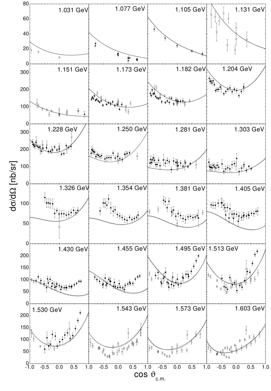
Figure 1: $\gamma p\rightarrow\gamma p$ differential cross section for different $\sqrt{s}$ as indicated in the figure. Calculation C-p$\gamma+$: solid line; C-p$\gamma-$: dashed line. Data are from Ref. datagg .

our calculations are able to describe the differential cross section in the considered energy region up to $\sqrt{s}=1.6$ GeV. Only in the intermediate energy region between 1.3 and 1.5 GeV are there indications of contributions missing in the present model. These missing contributions are due to the lack of $2\pi N$ rescattering contributions, since in the present model only resonant $2\pi N$ photoproduction mechanisms are included; see Sec. III. This leads to the lack of background contributions in the low energy two-pion photoproduction; see also the discussion in Sec. IV.7 below.

The same discrepancy in this energy region can also be observed in the $90^{\circ}$ region of the beam polarization (see Fig. 2),

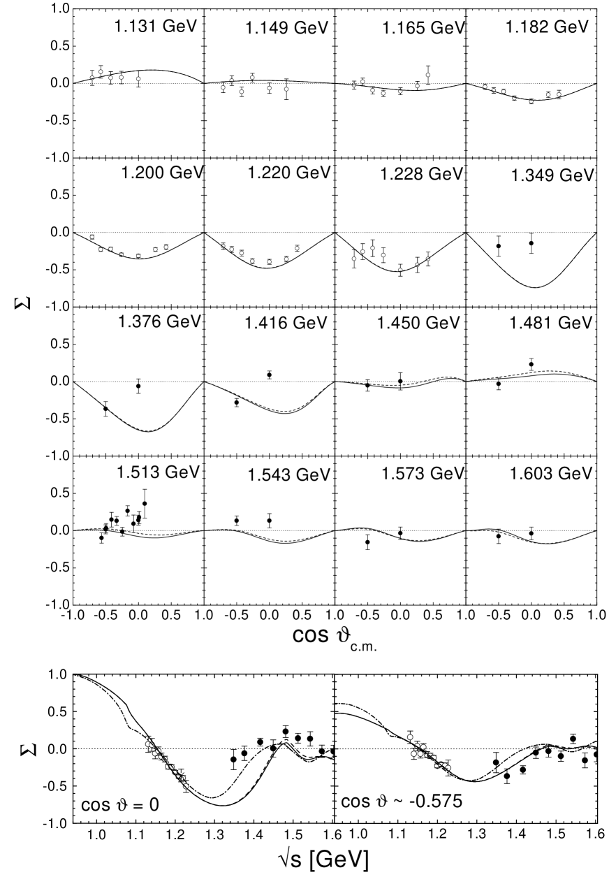
Figure 2: $\gamma p\rightarrow\gamma p$ differential beam polarization. Line code and data as in Fig. 1. In addition, the results of the analysis of L’vov et al. lvov are given by the dash-dotted line.

which is well described for energies below 1.3 and above 1.45 GeV and also other angles. For comparison, we also display the results on the beam polarization of the dispersion theoretical analysis of L’vov et al. lvov . In the model of Ref. lvov , analyticity constraints are taken into account by saturating $s$-channel dispersion relations with use of the VPI pion-photoproduction multipole analysis and resonance photocouplings. In addition, two-pion photoproduction background contributions are also taken into account. These authors’ description of the beam asymmetry is rather close to our description, with the exception of the above mentioned energy region and the $\pi N$ threshold region. This asserts the findings of Pearce and Jennings pearce , that, due to the extracted soft form factor, the off-shell rescattering contributions of the intermediate two-particle propagator in the scattering equation, which are neglected in the $K$-matrix approximation, have to be damped by a very soft form factor in $\pi N$ elastic scattering; see also PMI pm1 . Thus the effects of the off-shell rescattering part only become visible very close to the $\pi N$ threshold, in line with the above comparison of the present model with the dispersion theoretical analysis of L’vov et al. lvov . The cusp in the beam polarization at the $\pi N$ threshold is due to the ${\mathcal{T}}^{EE}_{1-}$ multipole amplitude [cf. Eq. (52)], which has also been found by Kondratyuk and Scholten kondratyuk .

As expected, the two global fits C-p-$\gamma\pm$ lead to practically identical results since Compton scattering is only considered up to 1.6 GeV, which is still far below the $\omega N$ threshold. The dominant contributions stem from the nucleon, the $P_{33}(1232)$ resonance, and the $D_{13}(1520)$, while the $P_{11}(1440)$ and $S_{11}(1535)$ only make small contributions.

IV.2 Pion photoproduction

Pion photoproduction is most precisely measured of all the channels considered in the present work. This has also led to the development of a large amount of models on this reaction (see references in Ref. feusti99 ), most of them concentrating on the low-energy [$P_{33}(1232)$] region. The Mainz MAID isobar model of Drechsel et al. maid covers a similar energy region as the present analysis. In MAID, the Born and vector meson background contributions were $K$-matrix unitarized with the help of the VPI $\pi N\rightarrow\pi N$ partial waves SM00 . Instead of using a form factor for the $\pi NN$ vertex, a pseudovector (PV)- pseudoscalar (PS) mixture scheme is introduced to regularize the nucleon contributions at higher energies. Since the resonance contributions are generated by unitarized Breit-Wigner descriptions, the resonances do not create additional background by $u$-channel diagrams. The advantage of this procedure is that the inclusion of spin-$\frac{5}{2}$ resonances is straightforward and, consequently, the $F_{15}(1680)$ is also taken into account. The free parameters (e.g., the vector meson couplings) are adjusted to the VPI multipoles SP01 and a very good description is achieved. As a consequence of the Breit-Wigner description and the restriction on pion photoproduction, the extracted electromagnetic helicity amplitudes of the resonances are very close to the Particle Data Group (PDG) values pdg , while in our analysis all resonance contributions are also constrained by Compton scattering, $\eta N$, $K\Lambda/\Sigma$, and $\omega N$ photoproduction data.

As a consequence of the precise experimental data, the pion-photoproduction channel is of great importance in our data base and contains about 40% of all data points, many of which have very small error bars. Thus this channels strongly influences the photon and pion couplings and also the masses of the resonances. For example, the masses of the $S_{11}(1535)$, $S_{31}(1620)$, $P_{31}(1750)$, and $D_{33}(1700)$ are influenced by the pion-photoproduction multipoles; see Figs. 3 – 5 and PMI pm1 .

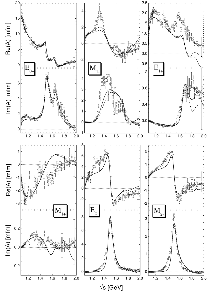
Figure 3: $\gamma N\rightarrow\pi N$ proton [see Eq. (55) in Appendix D.2] multipoles. Line code as in Fig. 1. Data are from the VPI SP01 single-energy ($\circ$) and energy-dependent ($\times$) solution.

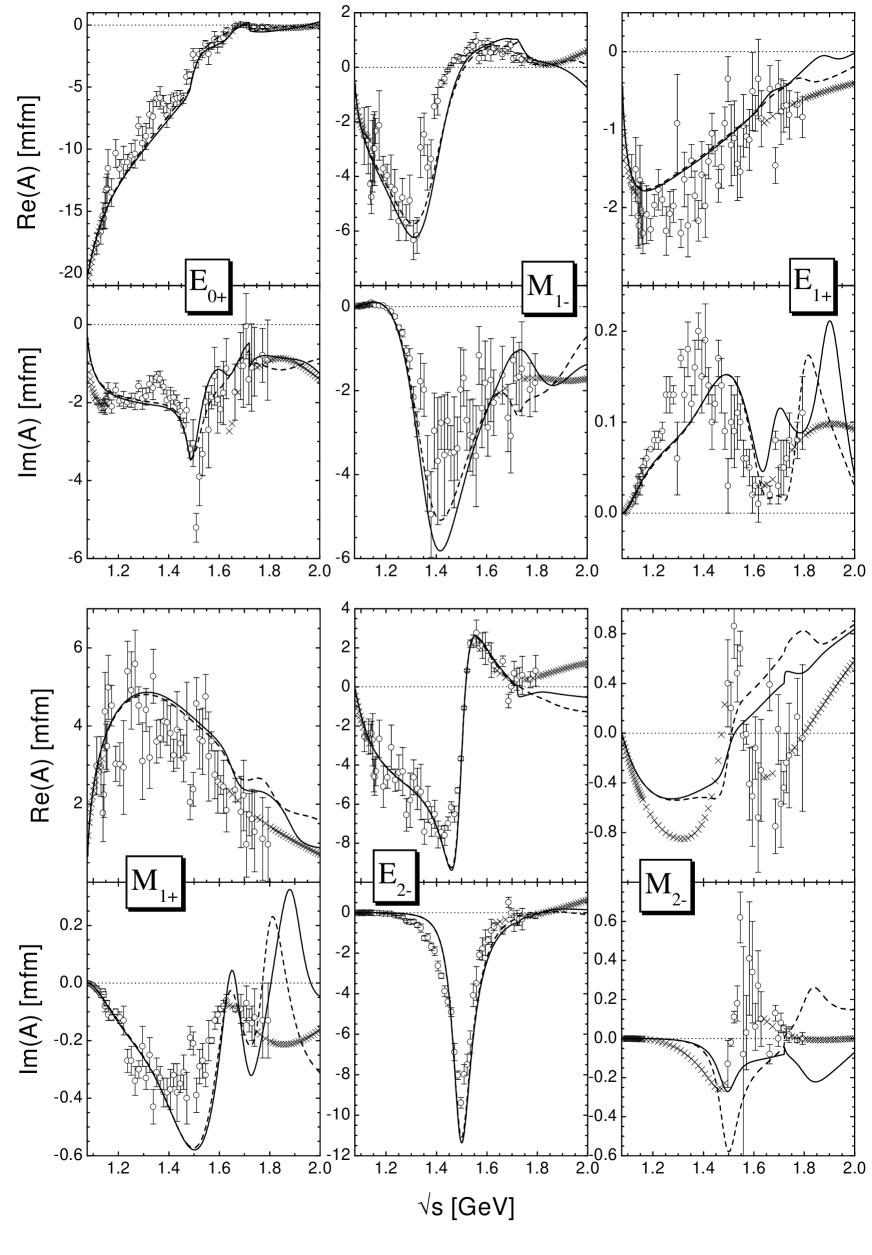
Figure 4: $\gamma N\rightarrow\pi N$ neutron [see Eq. (55) in Appendix D.2] multipoles. Line code as in Fig. 1, data as in Fig. 3.

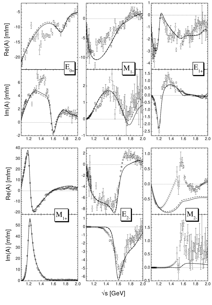
Figure 5: $\gamma N\rightarrow\pi N$ $I=\frac{3}{2}$ multipoles. Line code as in Fig. 1, data as in Fig. 3.

Although the resulting $\chi^{2}$ seems to be rather high ($\sim 10$), Figs. 3 $-$ 5 reveal, that the properties of almost all multipoles up to $J=\frac{3}{2}$ are well described in the present model.

The largest contributions to the total $\chi^{2}$ stem from the real parts of the $E_{1+}^{p}$, $E_{2-}^{p}$, $M_{1+}^{\frac{3}{2}}$, and $E_{2-}^{\frac{3}{2}}$ multipoles. In the latter three cases, this is a consequence of the fact, that around the resonances $D_{13}(1520)$, $P_{33}(1232)$, and $D_{33}(1700)$ the multipoles are known with very high accuracy, and thus even very small deviations in the calculation lead to a large $\chi^{2}$. For the $D_{13}(1520)$ multipoles $E_{2-}^{p/n}$ and $M_{2-}^{p}$, but also for the $D_{33}(1700)$ multipole $E_{2-}^{\frac{3}{2}}$, in the imaginary parts we observe the same problem of the increasing behavior below the resonance position as in the corresponding $\pi N$ partial waves (see PMI pm1 ), which is probably due to deficiencies in the present model concerning the $2\pi N$ final state description. In the case of the $E_{1+}^{p}$ multipole the deviation is due to the lack of some background contribution, which might be related to the problem in the description of the $\pi N\rightarrow\pi N$ $P_{13}$ partial wave described in PMI pm1 due to a missing ($3\pi N$) inelastic channel. It is interesting to note that the discrepancy between the calculation and the VPI data points in the $E_{1+}^{p}$ multipole starts around 1.6 GeV, which is the same energy, where the problems in the $P_{13}$ $\pi N\rightarrow\pi N$ wave arise, and also where a sudden increase in the total cross section of $\gamma p\rightarrow p\pi^{+}\pi^{-}\pi^{0}/n\pi^{+}\pi^{+}\pi^{-}$ was observed in experiments erbeom ; wisskirchen . For the neutron multipoles, there are only data of the energy-dependent solution available at energies above 1.8 GeV. Since these data are model dependent, they only enter with enlarged error bars in the present calculation, and the high-energy tails of the neutron multipoles are not well fixed. This explains the pronounced resonant structure in the imaginary part of the $E_{1+}^{n}$ and $M_{1+}^{n}$ multipoles, not observed in the VPI multipole data SP01 .

As can be seen in Figs. 3 $-$ 5, the differences between the two global calculations C-p-$\gamma+$ and C-p-$\gamma-$ can be mainly found in the $J^{P}=\frac{3}{2}^{+}$ proton and neutron multipoles above the $\omega N$ threshold. This is a consequence of the fact that these multipoles give important contributions to the $\omega N$ production mechanism (see Sec. IV.6 below and also the results on $\pi N\rightarrow\omega N$ in PMI pm1 ) and are thus very sensitive to the change of sign of the $t$-channel background contribution in $\pi N\rightarrow\omega N$.

Apart from the $E_{1+}^{p}$ multipole discussed above, we find indications for missing background only in the $M_{2-}^{n}$ and $M_{2-}^{\frac{3}{2}}$ multipoles, while in all other multipoles the background contributions seem to be in line with the VPI SP01 analysis. Since the background is mainly generated by the Born terms, the multipoles strongly influence the nucleon cutoff value $\Lambda_{N}$. In Fig. 6

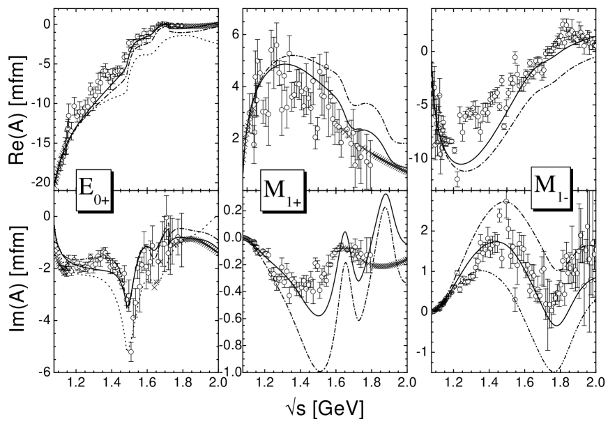
Figure 6: Examples for the influence of the nucleon cutoff value $\Lambda_{N}$ on the pion-photoproduction multipoles: neutron $E^{n}_{0+}$ (left), neutron $M^{n}_{1+}$ (middle), $I=\frac{3}{2}$ $M^{\frac{3}{2}}_{1-}$ (right). C-p-$\gamma+$ with $\Lambda_{N}=0.96$ GeV: solid line; C-p-$\gamma+$ with $\Lambda_{N}=1.16$ GeV: dash dotted line. For $E^{n}_{0+}$, also the calculation of Ref. feusti99 is displayed (dotted line). For the imaginary part of $M^{\frac{3}{2}}_{1-}$, the calculation C-p-$\gamma+$ using the Haberzettl gauging procedure is also shown (dash-double dotted line).

we show the sensitivity of the $E^{n}_{0+}$, $M^{n}_{1+}$, and $M^{\frac{3}{2}}_{1-}$ multipoles to the cutoff value $\Lambda_{N}$, which is used in the $\pi NN$ form factor. As we have pointed out in PMI pm1 , the $S_{11}$ and $P_{11}$ $\pi N\rightarrow\pi N$ partial waves are more poorly described once the pion-photoproduction data is included. This effect can be traced back to the necessity of reducing the value of $\Lambda_{N}=1.16$ GeV of the hadronic calculation to $\Lambda_{N}=0.96$ GeV in the global calculation. Using the latter value, the background contributions in the multipoles are in line with the VPI analysis SP01 , while with the former value the incorrect background description leads to largely increased $\chi^{2}$ values. The price one has to pay for the improvement in the mentioned multipoles is the deterioration in the low-energy $S_{11}$ and $P_{11}$ $\pi N$ elastic partial waves leading also to an increase of the $P_{11}(1440)$ mass and width. Since the Born terms are very sensitive to the gauging procedure, the resulting good description of most of the background features also indicates, that the Davidson-Workman gauging procedure [Eq. (15)] is supported by the pion-photoproduction data. As an example, we show the effect of switching to the Haberzettl gauging procedure [Eq. (16)] in the imaginary part of the $M_{1-}^{\frac{3}{2}}$ multipole in Fig. 6. Similar observations are also made in other multipoles. This is also related to the large $\chi^{2}$ improvement of the present calculation as compared to Ref. feusti99 , where the Haberzettl gauging procedure has been used. The largest differences as compared to Feuster and Mosel feusti99 can be observed in the real part of the $I=\frac{1}{2}$ $E_{0+}$ multipoles; see, e.g., $E^{n}_{0+}$ in Fig. 6. Note that it was already speculated in Ref. feusti99 , that modifying the gauging procedure might improve the description in these multipoles.

In the $M_{2-}^{\frac{3}{2}}$ multipole, in addition to the missing background mentioned above, also a too small resonance contribution is extracted in the present model. However, this contribution is also strongly constrained by the spin-$\frac{1}{2}$ off-shell contributions of the $D_{33}(1700)$ to the $E_{0+}^{\frac{3}{2}}$ and $M_{1-}^{\frac{3}{2}}$ multipoles. Since these multipoles are more precisely known than the $M_{2-}^{\frac{3}{2}}$ multipole, the fitting procedure is dominated by the background contributions of the $D_{33}(1700)$ in the spin-$\frac{1}{2}$ multipoles, resulting in photon couplings which deteriorate the $M_{2-}^{\frac{3}{2}}$ description.

IV.3 $\eta$ Photoproduction

Several investigations ben95 ; feusti99 ; sauermann showed, that the $\eta N$ photoproduction is dominated by a $J^{P}=\frac{1}{2}^{-}$ production mechanism, in particular at threshold. While we find in the pion-induced reaction still important $\frac{1}{2}^{+}$ and $\frac{3}{2}^{+}$ cross-section contributions, only a small contribution of the $P_{11}(1710)$ is visible in the photon-induced reaction, and the $\frac{1}{2}^{-}$ contribution is by far dominant up to 2 GeV, see Fig. 7.

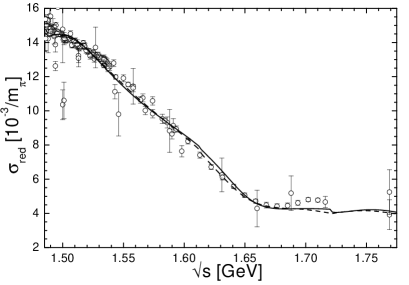
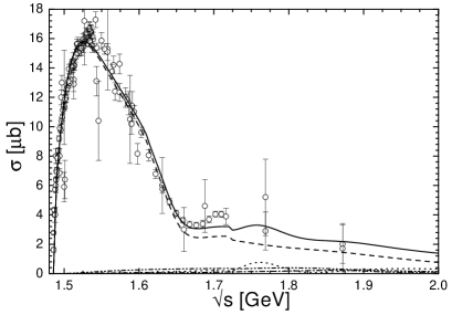
Figure 7: $\gamma p\rightarrow\eta p$. Data as given in Sec. III. Left: Reduced cross section. Line code as in Fig. 1. Right: Partial-wave decomposition of the total cross section, $J^{P}=\frac{1}{2}^{-}$: dashed; $\frac{1}{2}^{+}$: dotted; $\frac{3}{2}^{+}$: dash dotted; $\frac{3}{2}^{-}$: dash-double dotted.

Here we have also displayed the so-called reduced cross section, which takes out effects caused by phase space and is given by $\sigma_{red}=\sqrt{\sigma_{tot}\>\>\!\!{\mathrm{k}}/(4\pi\>\>\!\!{\mathrm{k}}^{\prime})}$ (cf. Appendix E), and allows for more conclusive investigations close to threshold. As can be clearly seen in Fig. 7, the production mechanism is well under control in the present model down to the very threshold. Thus the energy dependence of the $\eta N$ total cross section is correctly described, although the inclusion of the pion photoproduction $E_{0+}^{p}$ multipole data requires a reduction of the $S_{11}(1535)$ mass from $\approx 1.544$ to $\approx 1.526$ GeV; see also PMI pm1 . Note that our calculations do not follow the increase of the GRAAL total cross section datage around 1.7 GeV, which is not observed in the estimated total cross section from the CLAS collaboration dugger either.

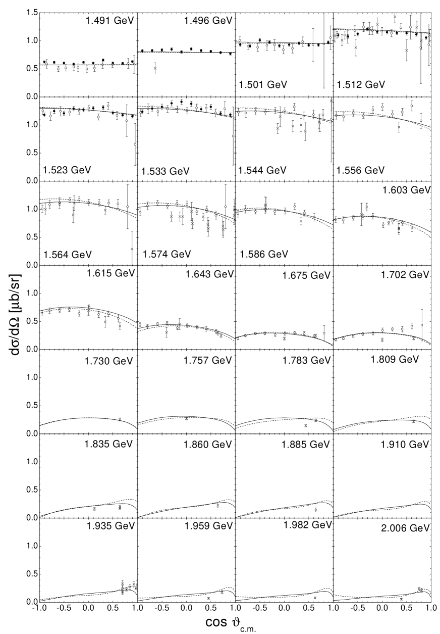
Figure 8: $\gamma p\rightarrow\eta p$ differential cross section. Line code as in Fig. 1. Data are as given in Sec. III. The data from Ref. dugger are not shown.

In the first coupled-channel model on photon- and pion-induced $\eta N$ production up to $\sqrt{s}=1.75$ GeV by Sauermann et al. sauermann , it has been found, that an important production mechanism is due to the vector meson ($\rho$ and $\omega$) exchanges. In line with these authors’ findings, it also turns out in the present model that these exchanges give important contributions in all partial waves and the neglect would lead to total cross sections below the experimental data already at 1.55 GeV. Note that in the present calculation the forward peaking behavior of the differential cross section at higher energies is less pronounced as compared to Ref. feusti99 (see Fig. 8),

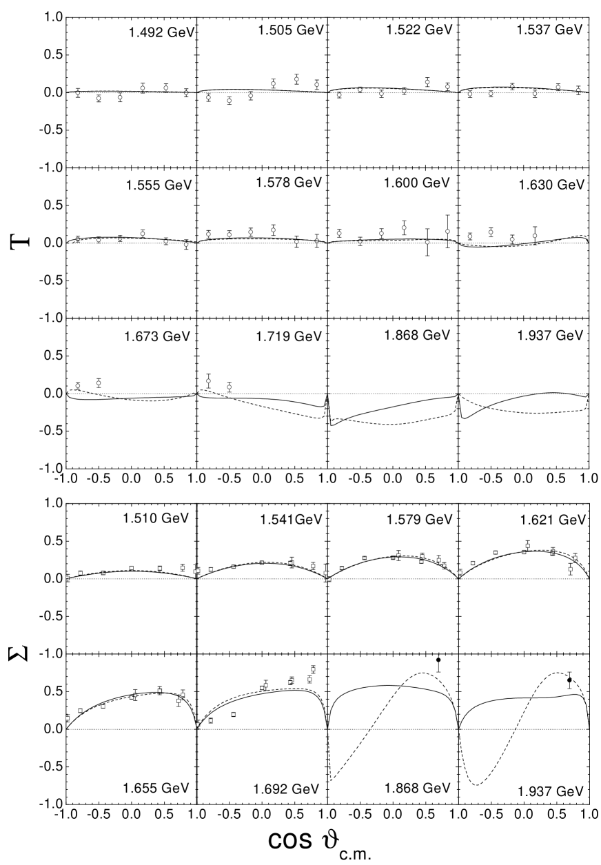
Figure 9: $\gamma p\rightarrow\eta p$ target- (upper panel) and beam- (lower panel) polarization measurements. Line code as in Fig. 1. Data are as given in Sec. III.

which is in line with the preliminary CLAS dugger and the older experimental data.

The resulting decomposition of the $\eta N$ photoproduction describes the differential cross sections and polarization measurements very well in the complete considered energy region; see Figs. 8 and 9. As pointed out in Sec. III prior to the differential cross section measurements of the CLAS Collaboration dugger , there were hardly any measurements taken above 1.7 GeV. Consequently, the preliminary CLAS data give strong constraints on the reaction mechanism in the upper energy region, which would otherwise be mainly determined by the pion-induced $\eta N$ data being of poor quality at higher energies; see PMI pm1 .

It is interesting to note that we find a considerably smaller $D_{13}(1520)$ $\eta N$ width than, e.g., Batinić et al. batinic . However, since the $D_{13}(1520)$ basically gives the only contribution to the low energy behavior of the beam polarization $\Sigma$ feusti99 , our value of around 20 KeV (as compared to 140 KeV) is strongly corroborated by the measurements of the GRAAL collaboration datage , since these data are very well described in the complete measured region; see Fig. 9. Note also that Tiator et al. tiator99 deduced from the GRAAL beam asymmetry data a $D_{13}(1520)$ $\eta N$ branching ratio of $0.8\pm 0.1$‰, which is about half of our value. This is related to the fact, that in these authors’ analysis, the PDG pdg electromagnetic helicity amplitudes have been used, which are larger than the ones deduced from our analysis; see Table 7 below. In Ref. tiator99 it was also shown, that the forward-backward asymmetry of the beam polarization $\Sigma$ between 1.65 and 1.7 GeV (see Fig. 9) can only be explained by contributions with spin $J\geq\frac{5}{2}$. Since in the present model no $J\geq\frac{5}{2}$ resonances are included, the asymmetric behavior is generated by the vector meson exchanges. Since the GRAAL data cannot be completely described at 1.69 GeV, this might be an indication that spin-$\frac{5}{2}$ resonances indeed play a role in $\eta N$ photoproduction. At higher energies ($\sqrt{s}>1.8$ GeV), an opposite behavior of the beam asymmetry for our two calculations at backward angles is observed. Since there are no data points, only the behavior at forward angles is fixed. The difference in the two calculations can be explained by the opposite photon helicity amplitudes of the $D_{13}(1950)$ (see Table 7 in Sec. IV.9 below) and the different $\eta N$ strength (5.4% for C-p-$\gamma+$ and 8.6% C-p-$\gamma-$). Thus beam-asymmetry measurements at energies above 1.7 GeV for $\eta N$ photoproduction would be a great tool to study the properties of this “missing” resonance and also the necessity for the inclusion of a spin-$\frac{5}{2}$ resonance in more detail.

For the target polarization, we find small values in the complete energy region; see Fig. 9. Only in the lowest energy bins, the experimental data seem to indicate a nodal structure. Tiator et al. tiator99 showed, that this behavior can only be explained by a strong energy dependence of the relative phase between the $S_{11}(1535)$ and $D_{13}(1520)$ contributions, which is not found in the present calculation. For the region above 1.6 GeV, our calculations change from positive to negative values, which seems not to be supported by the Mainz data datage at backward angles. It turns out that the target polarization is dominated in our calculation by the $P_{11}(1710)$ resonance properties, and, hence, more experimental data on the target polarization at higher energies would also help to clarify whether this resonance plays such an important role in $\eta N$ photoproduction as found in the present analysis.

IV.4 $K\Lambda$ photoproduction

The decomposition of the $K\Lambda$ photoproduction channel turns out to be very similar to the pion-induced reaction. In contrast to Feuster and Mosel feusti99 , where the $S_{11}(1650)$ and the $P_{11}(1710)$ dominated this reaction, in the present calculation the former one turns out to be important only very close to threshold, while the latter one hardly gives any sizeable contribution at all; see Fig. 10.

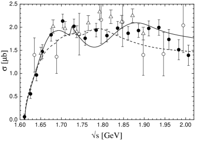
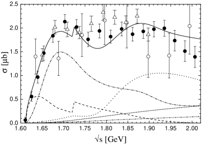
Figure 10: $\gamma p\rightarrow K^{+}\Lambda$ total cross section. Data are as given in Sec. III. Left: Line code as in Fig. 1. Right: Partial-wave decomposition. Notation as in Fig. 7. In addition, the contribution of higher partial waves ($J\geq\frac{5}{2}$) is indicated by the short-dashed line.

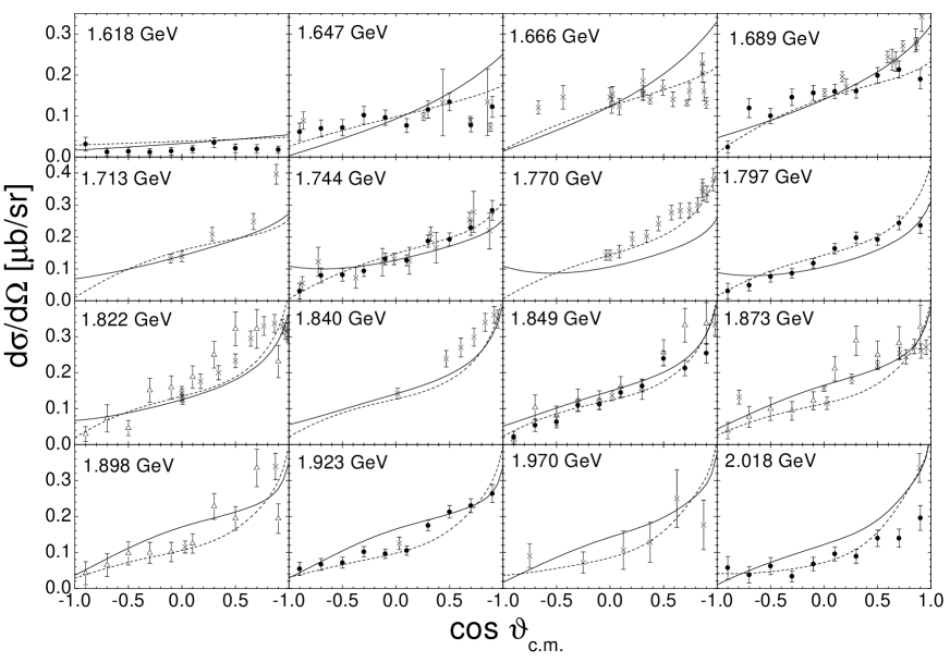
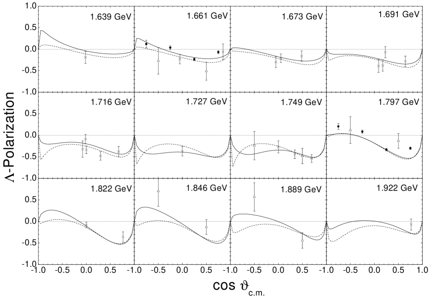
Figure 11: $\gamma p\rightarrow K^{+}\Lambda$ differential cross section (upper panel) and $\Lambda$-recoil polarization (lower panel). Line code as in Fig. 1. Data are as given in Sec. III.

At low energies, the $P_{13}(1720)$ ($J^{P}=\frac{3}{2}^{+}$) resonance is dominating, causing a resonant structure around 1.7 GeV. At higher energies, the $P_{13}(1900)$ still makes important contributions due to rescattering in spite of its small $K\Lambda$ width. The strong $\frac{1}{2}^{-}$ contribution very close to threshold, which is caused by the $S_{11}(1650)$, is strongly influenced by the $\omega N$ threshold leading to a sudden increase in the total cross section. Note, that the finite width of the $\omega$ meson of 8 MeV, which is not taken into account in the present model, smears out this threshold effect. A similar observation of the feeding of $K\Lambda$ (and also $K\Sigma$, see Sec. IV.5 below) photoproduction through threshold effects has also been made in the coupled-channel model of Lutz et al. lutz . As a consequence of the inclusion of the $K^{*}$ and $K_{1}$ meson exchanges, we also find important contributions to the total cross section by partial waves with $J\geq\frac{5}{2}$, cf. Fig. 10.

A striking difference to the pion-induced $K\Lambda$ production mechanism is observed in the $\frac{1}{2}^{+}$ wave, which exhibits a structure resonating around 1.9 GeV, where a second peak is also visible in the SAPHIR total cross section data datagl . However, there is no $P_{11}$ resonance included in the present model around this energy. It turns out that the $\frac{1}{2}^{+}$ behavior is caused by the interference of the nucleon and $K^{*}$ contributions. Switching these two contributions off leads to a $\frac{1}{2}^{+}$ wave, which is practically zero for energies higher than the $P_{11}(1710)$ peak. This is in contrast to the findings of the single-channel model of Mart and Bennhold martbenn , where the peaking behavior in the SAPHIR total cross section datagl was explained by the same $D_{13}(1950)$ resonance, which was found by Feuster and Mosel feusti98 ; feusti99 around 1.9 GeV. This example emphasizes the importance of coupled-channel analyses for the correct identification of missing resonances. Although the $D_{13}(1950)$ is included in the present calculation, in the simultaneous analysis of all channels it turns out to be of negligible importance for $K\Lambda$ photoproduction. Similar results were already found by Janssen et al. janssen01 . Using a field-theoretic model, these authors deduced that the present $K\Lambda$-photoproduction data alone are insufficient to identify the exact properties of a missing resonance in a single-channel analysis on $K\Lambda$ photoproduction. Moreover, these properties also depend on the background contributions. Since in the present model the background is uniformly generated for the various reaction channels, and pion- and photon-induced data are analyzed simultaneously, the extracted background and resonance contributions are more strongly constrained than in Ref. martbenn , and more reliable conclusions can be drawn.

The recoil polarization (see Fig. 11) is equally well described in the two global calculations C-p-$\gamma+$ and C-p-$\gamma-$, although the difference in the $g_{\omega\rho\pi}$ sign leads to changes in the $P$-wave resonance couplings. However, since the differential cross section displayed in Fig. 11 is $P$-wave dominated, slight changes in the forward peaking and backward decrease can be seen in this observable. This different behavior is the reason for the better $\chi^{2}$ value of C-p-$\gamma-$ as compared to C-p-$\gamma+$, and again shows, that $K\Lambda$ production reacts very sensitive on rescattering effects due to $\omega N$.

As a consequence of the inclusion of the photoproduction data, the $NK\Lambda$ coupling is only reduced from $-18.8$ to $-12.2$ from the best hadronic (C-p-$\pi+$; see PMI pm1 ) to the best global (C-p-$\gamma+$) fit (see also Table 5 in Sec. IV.8 below). Thus, in contrast to other models on $K\Lambda$ photoproduction, the resulting agreement of the present calculation with experimental data is neither achieved with a very low $NK\Lambda$ coupling far off SU(3) predictions, nor with a very soft nucleon form factor; see Table 6 in Sec. IV.8. Note that the same cutoff value $\Lambda_{N}=0.96$ GeV is used in all nucleon $s$- and $u$-channel diagrams.

IV.5 $K\Sigma$ Photoproduction

As it turns out in the present model, it is also possible to simultaneously describe both measured $\gamma p\rightarrow K\Sigma$ charge reactions (see Table 3 and Fig. 12), while still being in line with all three pion-induced $K\Sigma$ charge channels (see Table 2 and PMI pm1 ). Similarly to $K\Lambda$ photoproduction, the $K\Sigma$ mechanism also proves to be very sensitive to rescattering effects via $\omega N$. The $IJ^{P}=\frac{1}{2}\frac{1}{2}^{-}$ $K\Sigma$ wave is fed by the $\omega N$ channel, leading to a sudden increase in the $K^{+}\Sigma^{0}$ and $K^{0}\Sigma^{+}$ total cross sections. As pointed out in Sec. IV.4, such an effect has also been observed in the coupled-channel model of Lutz et al. lutz . Note that the finite width of the $\omega$ meson of 8 MeV, which is not taken into account in the present model, smears out this threshold effect.

Fit	Total $\chi^{2}_{\gamma\Sigma}$	$\chi^{2}(\gamma p\rightarrow K^{+}\Sigma^{0})$	$\chi^{2}(\gamma p\rightarrow K^{0}\Sigma^{+})$
C-p-$\gamma+$	2.74	2.81	2.38
C-p-$\gamma-$	2.27	2.28	2.17

Table 3: Resulting $\chi^{2}$ of the two global fits for the two different charge reactions in $\gamma p\rightarrow K\Sigma$.

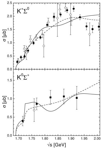
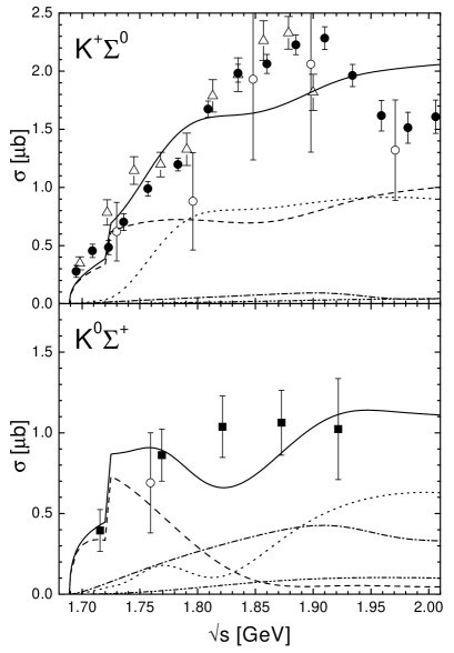
Figure 12: $\gamma p\rightarrow K\Sigma$ total cross sections. Data are as given in Sec. III. Left: Line code as in Fig. 1. Right: Partial-wave decomposition. Line code as in Fig. 7.

The total cross section of $\gamma p\rightarrow K^{+}\Sigma^{0}$ is dominantly composed of $J^{P}=\frac{1}{2}^{-}$ and $\frac{1}{2}^{+}$ contributions, where the latter is generated by the $P_{31}(1750)$ and $K^{*}$ exchange contributions. The higher partial waves, especially those with $J\geq\frac{5}{2}$, hardly play any role. In the $\gamma p\rightarrow K^{0}\Sigma^{+}$ reaction, the situation is changed in such a way that the contribution of the $P_{11}(1710)$ becomes more pronounced, and the the $J^{P}=\frac{3}{2}^{+}$ contribution due to the $P_{33}(1920)$ and in particular the $P_{13}(1900)$ is emphasized. The $J^{P}=\frac{3}{2}^{-}$ and higher partial-wave contributions remain negligible. A similar decomposition of the $K\Sigma$-photoproduction mechanism was found by Janssen et al. janssen02 . By applying a tree-level isobar model, these authors were able to exclude any relevance of the $D_{13}$ wave and to identify important contributions from the $P_{11}(1710)$ and $S_{11}(1650)$ as in our model. Also $P_{13}$, $S_{31}$, and $P_{31}$ contributions have been identified, however, those have been attributed to the $P_{13}(1720)$, $S_{31}(1900)$, and $P_{31}(1910)$ resonances instead of $P_{13}(1900)$, $S_{31}(1620)$, and $P_{31}(1750)$ in the present model. Note, that we have checked for the importance of $S_{31}(1900)$ and $P_{31}(1910)$ contributions within the present model (see PMI pm1 ), but have not found any sizable contributions.

The differential cross section behavior of $\gamma p\rightarrow K^{+}\Sigma^{0}$, shown in Fig. 13,

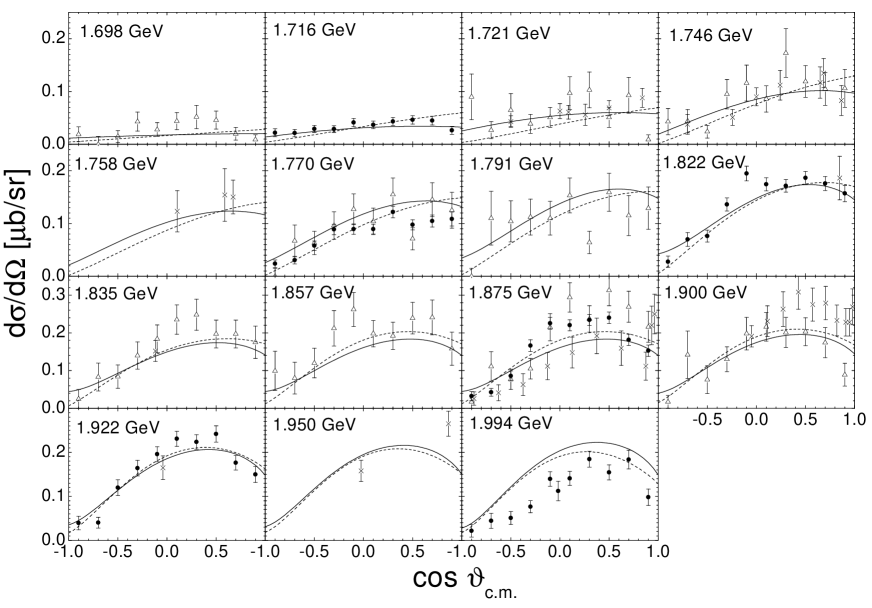
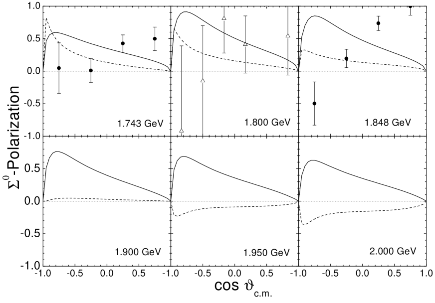
Figure 13: $\gamma p\rightarrow K^{+}\Sigma^{0}$. Upper panel: differential cross section, lower panel: $\Sigma^{0}$-recoil polarization. Line code as in Fig. 1. Data are from Ref. datags .

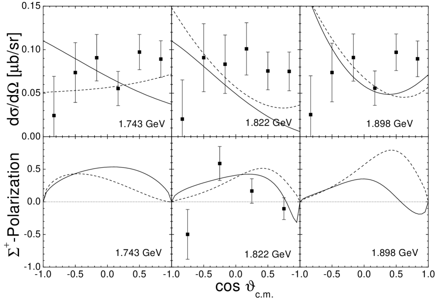
Figure 14: $\gamma p\rightarrow K^{0}\Sigma^{+}$ differential cross section and $\Sigma^{+}$ recoil polarization. Line code as in Fig. 1. Data are from Ref. datags .

is very similar for the two global calculations C-p-$\gamma\pm$ with different coupling signs of $g_{\omega\rho\pi}$. Both describe the angular structure of the cross sections very well and show a tendency to decrease at forward angles for higher energies, which is caused by the $K^{*}$ exchange. In the $\Sigma^{0}$ recoil polarization of $\gamma p\rightarrow K^{+}\Sigma^{0}$, the two calculations C-p-$\gamma+$ and C-p-$\gamma-$ show behaviors opposite in sign for energies above 1.9 GeV. This difference can be traced back to the different $P_{11}(1440)$, $P_{11}(1710)$, and $D_{13}(1950)$ contributions in the two calculations. Thus more precise experimental data in the higher-energy region on the $\Sigma^{0}$ polarization would certainly help to clarify the exact decomposition.

We also observe a very similar behavior of the two calculations for the $\gamma p\rightarrow K^{0}\Sigma^{+}$ (see Fig. 14) differential cross section and $\Sigma^{+}$ polarization. Unfortunately, the few SAPHIR data points datags are not precise enough to judge the quality of the description.

As a result of the inclusion of the photoproduction data, the $NK\Sigma$ coupling is reduced from 15.4 to 2.5 from the best hadronic (C-p-$\pi+$) to the best global (C-p-$\gamma+$) fit. As pointed out in Sec. IV.8 and PMI pm1 , the pion- induced reactions are only slightly influenced by the exact $NK\Sigma$ coupling value and are thus still be well described in the global calculation. The final value for the $NK\Sigma$ coupling is close to SU(3) expectations; see Sec. IV.8.

IV.6 $\omega$ photoproduction

The literature on $\omega$ photoproduction does not offer a clear picture of the importance of individual resonance mechanisms in this channel, which is due to the fact that basically all models are only single-channel analyses. Hence rescattering effects and the impact of the drawn conclusions on other channels are neglected. While Titov and Lee titov02 recently found important contributions of the sub-threshold $D_{13}(1520)$ and $F_{15}(1680)$ resonances, Oh et al. oh01 extracted dominant contributions from a $P_{13}(1900)$ and a $D_{13}(1960)$ resonance. Furthermore, in the model of Zhao zhao01 the $P_{13}(1720)$ and $F_{15}(1680)$ were shown to give dominant contributions, but the low lying $S_{11}(1535)$ and $D_{13}(1520)$ were also important. All models agree, however, on the importance of the $\pi^{0}$ exchange, which has already been considered in one of the first models on $\omega$ photoproduction by Friman and Soyeur frimansoyeur . The higher partial-wave contributions of the $\pi^{0}$ mechanism also dominate the cross section behavior above $\sqrt{s}\approx 1.82$ GeV in the present model; see Fig. 15.

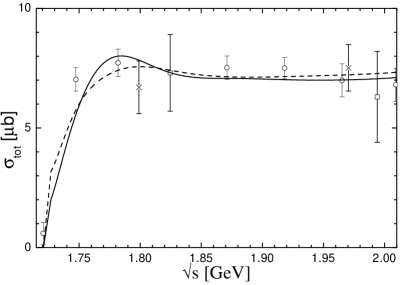
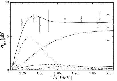
Figure 15: $\gamma p\rightarrow\omega p$ total cross section. Data are from $\circ$ kleingo , $\times$ erbeom , $\Box$ crouch . The data from Ref. barthom are not shown. Left: Line code as in Fig. 1. Right: Partial-wave decomposition. Notation as in Fig. 10.

The clear dominating threshold contribution stems from the $P_{11}(1710)$, just as in the pion-induced case (see PMI pm1 ). The importance of the other resonances, however, is reduced, and only the $J^{P}=\frac{3}{2}^{+}$ contributions of the $P_{13}(1720)$ and $P_{13}(1900)$ remain non-negligible.

The dominance of the $\pi^{0}$ exchange mechanism becomes even more obvious in the differential cross section; see Fig. 16.

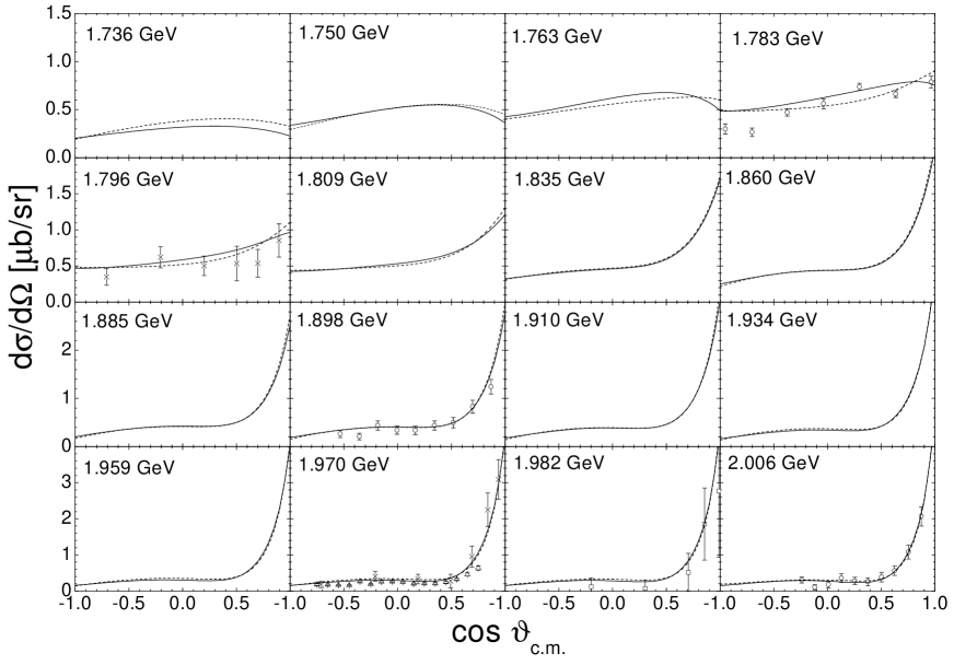
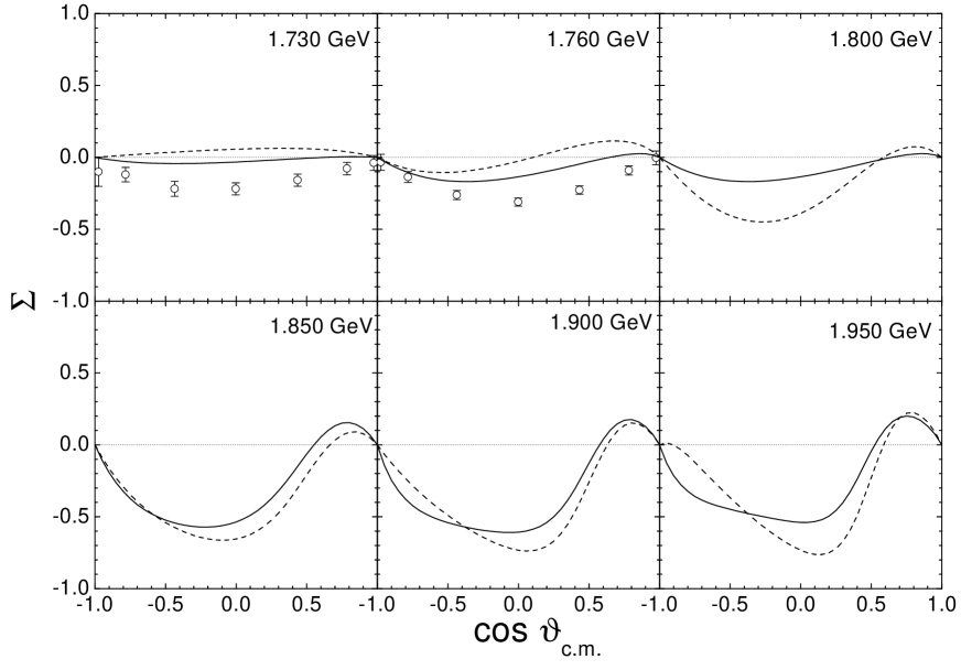
Figure 16: $\gamma p\rightarrow\omega p$. Line code as in Fig. 1. Upper panel: differential cross section. Data are as in Fig. 15. The preliminary CLAS data manak ($\triangle$) have not been used in the fitting procedure. Lower panel: Beam asymmetry $\Sigma$. Preliminary data are from Ref. ajakago .

However, in particular in the middle- and backward-angle region the resonance contributions destructively interfering with the pion exchange are mandatory to describe the precise preliminary SAPHIR data barthom , which cover the complete angular range. When these resonance contributions are neglected, the total cross section behavior is strongly altered and the calculation largely overestimates the total cross section; see Fig. 17.

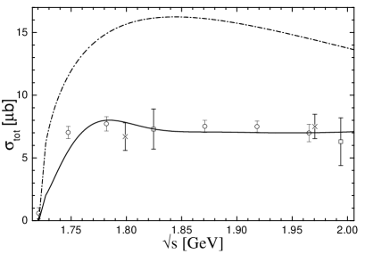
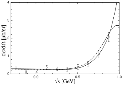
Figure 17: $\gamma p\rightarrow\omega p$. Data as in Fig. 15. Left: total cross section. Solid line: full calculation C-p-$\gamma+$. Dash-dotted line: C-p-$\gamma+$ with resonance contributions switched off. Right: Solid line: full calculation C-p-$\gamma+$. Dash-dotted line: C-p-$\gamma+$ with $J_{max}=\frac{11}{2}$; see the text.

The upper limit of the partial-wave decomposition $J_{max}$ turns out to be essential for the $\omega$ photoproduction channel because of the importance of the pseudoscalar $\pi^{0}$ exchange. Performing the decomposition only up to $J_{max}=\frac{11}{2}$ as in Refs. feusti98 ; feusti99 , the full upward bending behavior at forward angles is not reproduced. This is displayed in Fig. 17. We have checked for $J_{max}$ providing good convergence in the angular structure and found a satisfying behavior for $J_{max}\approx\frac{27}{2}$, which is consequently used in the partial-wave decomposition for the present calculation. The necessity of the consideration of higher partial waves when pseudoscalar exchange mechanisms are included was also pointed out recently by Davidson and Workman davidson01b . These authors demonstrated striking differences in the forward peaking behavior for a pion-photoproduction calculation at 1.66 GeV using the VPI multipoles only up to $\ell_{\pi}=5$ ($\Leftrightarrow J_{max}=\frac{11}{2}$) or additionally taking into account the full angular structure of the Born terms, in particular the pion-Bremsstrahlung contribution.

Although the inclusion of the precise SAPHIR photoproduction data barthom allows for a better disentangling of the importance of different resonances, the various resonance (helicity) couplings to $\omega N$ cannot be fixed with certainty; see PMI pm1 . To clarify the situation, there is an urgent need for data on polarization observables of $\omega N$ photoproduction, as, e.g., currently extracted at GRAAL. For comparison, we give our results on the beam asymmetry $\Sigma$ in Fig. 16. Note that the preliminary GRAAL data ajakago have not yet been included in the fit.

IV.7 Photoabsorption on the nucleon

In the present model, we have included all important inelastic $\pi N$ channels below $\sqrt{s}=2$ GeV, and, hence, we can also compare the resulting total photoabsorption cross section $\sigma_{abs}^{T}=\frac{1}{2}(\sigma^{\frac{1}{2}}_{abs}+\sigma^{\frac{3}{2}}_{abs})$ on the proton with experimental data armstrong ; maccormick . As can be seen from Fig. 18

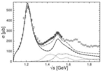
Figure 18: Total photoabsorption cross section on the proton $\gamma p\rightarrow X$. Calculation C-p-$\gamma+$: solid line; C-p-$\gamma-$: dashed line; cross section $\Delta\sigma$ of Ref. lvov (see the text): dotted line; sum of calculation C-p-$\gamma+$ and $\Delta\sigma$: dash-dotted line; $\gamma p\rightarrow 2\pi N$ of C-p-$\gamma+$: dash-double-dotted line (see the text). Data are from $\times$ maccormick and $\circ$ armstrong .

our model is in line with experiment all through the $\Delta(1232)$ region, but we cannot describe the total photoabsorption cross section $\sigma_{abs}^{T}$ above the $2\pi N$ threshold. This is not unexpected: the photoproduction of $2\pi N$ cannot be described within our model as well as the pion-induced $2\pi N$ production, since in the photon-induced reaction, e.g., $\rho N$ or $\pi\Delta$ contact (Kroll-Rudermann like) interactions are also known to be important hirata ; murphy ; oset .

In the dispersion theoretical analysis of Compton scattering by L’vov et al. lvov , exactly this part of the total photoabsorption cross section has been determined. By subtracting from the experimental total photoabsorption cross section $\sigma_{abs}^{T}=\frac{1}{2}(\sigma^{\frac{1}{2}}_{abs}+\sigma^{\frac{3}{2}}_{abs})$ on the proton armstrong ; maccormick the single-pion photoproduction cross section, determined via the VPI multipoles, and their $2\pi N$ cross section simulated via nucleon resonances, they extracted a remaining cross section $\Delta\sigma$ supposed to be due to the aforementionned background interactions. Ignoring interference effects (see Ref. lvov ), one can just add $\Delta\sigma$ to our total photoabsorption cross section. The resulting sum is remarkably close to the experimental photoabsorption cross section armstrong ; maccormick up to about 1.6 GeV (see Fig. 18), above which important contributions of spin-$\frac{5}{2}$ resonances can be expected, which are so far missing in our analysis. Thus it seems that the resonance contributions to the $2\pi N$ photoproduction, displayed in Fig. 18 by the dash-double-dotted line, are rather well described within the present model. This provides an additional cross check that at least up to 1.6 GeV all important channels are correctly described in our model. Above 1.6 GeV the data of the ABBHHM Collaboration on $3\pi N$ photoproduction erbeom indicate that this channel contributes $\approx 30-40$ $\mu$b to $\sigma^{T}_{abs}$, less than 10 $\mu$b of which are due to $\omega N$.

Realizing the limitations of the present model, we can nevertheless give estimates on the contributions of the various final states to the Gerasimov-Drell-Hearn (GDH) sum rule gdh (see also Ref. drechsel and references therein), which allows one to relate the static property of the anomalous magnetic moment of the nucleon to the photoabsorption cross section difference $\sigma^{\frac{1}{2}}_{abs}-\sigma^{\frac{3}{2}}_{abs}$ via dispersion relations. The contributions of the individual reactions on the proton target up to $\sqrt{s}=2$ GeV are given in Table 4.

$\;\;\pi N$	$2\pi N$	$\;\eta N$	$\;K\Lambda$	$\;K\Sigma$	$\;\omega N$
$-157.5$	$-21.2$	$\;\>+9.2$	$+1.1$	$+1.6$	$+0.8$
$-162.7$	$-20.7$	$\;\>+8.6$	$+0.9$	$+1.8$	$+0.1$
$-171^{a}$	$-45^{a}$	$+15^{a}$	$+1.7^{b}$	$+2.4^{b}$	$-2.0^{c}$

Table 4: Contributions (in $\mu$b) of the individual final states to the GDH sum rule up to $\sqrt{s}=2$ GeV on the proton target. First line: Calculation C-p-$\gamma+$; second line: C-p-$\gamma-$; third line: Values are from Refs. ^a: tiatorgdh , ^b: sumowidagdo , and ^c: zhao02 .

As is clear from the above discussion, our estimates for $\pi N$ and $2\pi N$ deviate from the rather well known values for reasons well understood. For all other final states ($\eta N$, $K\Lambda$, $K\Sigma$, and $\omega N$) our model is compared to all available experimental observables and thus allows for reasonable estimates of the contributions to the GDH sum rule. It is interesting to note (see Table 4) that our values for the contributions from $\eta N$, $K\Lambda$, $K\Sigma$, and in particular $\omega N$ deviate from the values of Refs. tiatorgdh ; sumowidagdo ; zhao02 , all of which have been extracted in single-channel analyses.

IV.8 Born and background couplings

The values of all Born and background couplings of our two global fits and the extracted cutoff values $\Lambda$ are summarized in Tables 5 and 6.

$g$	Value	$g$	Value	$g$	Value	$g$	Value
$g_{NN\pi}$	12.85	$g_{NN\sigma}\cdot g_{\sigma\pi\pi}$	$11.46$	$g_{NN\rho}$	4.53	$\kappa_{NN\rho}$	1.47
	12.75		$12.57$		4.40		1.41
$g_{NN\eta}$	0.10	$g_{NNa_{0}}$	$-35.30$	$g_{NN\omega}$	3.94	$\kappa_{NN\omega}$	$-0.94$
	0.12		$-22.91$		3.87		0.17
$g_{N\Lambda K}$	$-12.20$	$g_{N\Lambda K_{0}^{*}}$	26.27	$g_{N\Lambda K^{*}}$	$-27.61$	$\kappa_{N\Lambda K^{*}}$	$-0.50$
	$-12.88$		$1.16$		$-28.29$		$-0.55$
$g_{N\Sigma K}$	2.48	$g_{N\Sigma K_{0}^{*}}$	$-26.15$	$g_{N\Sigma K^{*}}$	4.33	$\kappa_{N\Sigma K^{*}}$	$-0.86$
	1.56		$-27.22$		3.88		$-0.98$
$g_{N\Lambda K_{1}}$	$-19.20$	$\kappa_{N\Lambda K_{1}}$	$-1.83$	$g_{N\Sigma K_{1}}$	$22.80$	$\kappa_{N\Sigma K_{1}}$	$2.40$
	$-24.35$		$-1.99$		23.29		2.06

Table 5: Nucleon and $t$-channel couplings. First line: C-p-$\gamma+$; second line: C-p-$\gamma-$.

$\Lambda_{N}$ [GeV]	$\Lambda^{h}_{\frac{1}{2}}$ [GeV]	$\Lambda^{\gamma}_{\frac{1}{2}}$ [GeV]	$\Lambda^{h}_{\frac{3}{2}}$ [GeV]	$\Lambda^{\gamma}_{\frac{3}{2}}$ [GeV]	$\Lambda^{h}_{t}$ [GeV]
0.96	4.00	1.69	0.97	4.30	0.70
0.96	4.30	1.59	0.96	4.30	0.70

Table 6: Cutoff values for the form factors. First line: C-p-$\gamma+$; second line: C-p-$\gamma-$. The upper index $h$ or $\gamma$ denotes whether the value is applied to a hadronic or electromagnetic vertex, while the lower one denotes the particle going off-shell, i.e., $N$: nucleon; $\frac{1}{2}$: spin-$\frac{1}{2}$ resonance; $\frac{3}{2}$: spin-$\frac{3}{2}$ resonance; $t$: $t$-channel meson.

Since these values were already discussed in PMI pm1 , we only outline the main properties.

When realizing that the values of $g_{\pi NN}$ are lower than the values extracted by other groups, for example the value of $g_{\pi NN}=13.13$ from the VPI group SM00 , one has to keep in mind that the present calculation considers a large energy region using only one $\pi NN$ coupling constant, and that the $\pi NN$coupling is especially influenced by the $t$-channel pion exchange mechanism of $\omega N$ photoproduction. Remember that only one cutoff value $\Lambda_{t}=0.7$ GeV (see Table 6) is used for all $t$-channel diagrams. As a result of gauge invariance, the importance of the Born diagrams is enhanced in the photoproduction reactions and consequently, the other Born couplings can also be more reliably extracted in the global calculations than when just the pion-induced data is considered. As found in previous analyses sauermann ; feusti98 ; feusti99 the $\eta NN$ coupling turns out to be very small and the precise value thus hardly influences the $\chi^{2}$ of the $\eta N$ production. The $K\Lambda$ and $K\Sigma$ couplings turn out to be larger than extracted in other calculations. Thus the resulting relations between the Born couplings for the pseudoscalar mesons of our best global fit are actually close to SU(3) relations with $\alpha_{FD}=F/(F+D)\in[0.25;0.41]$ (see, e.g., Ref. dumbrajs ), which is around the value o $\alpha_{FD}\approx 0.35$ predicted by the Cabibbo-theory of weak interactions and the Goldberger-Treiman relation dumbrajs . Furthermore, the $\omega NN$ coupling constants are also larger than extracted in other calculations, which is only possible since rescattering effects are properly taken into account in the present model. Note, that our value for the nucleon cutoff $\Lambda_{N}=0.96$ GeV (see Table 6) is the same for all final states.

The only $t$-channel meson which exclusively contributes to photoproduction reactions in the present model, is the $K_{1}$ meson. Although the couplings are almost identical in both calculations, we find that it only plays a minor role in $K\Lambda$ and $K\Sigma$ photoproduction; far more important are the contributions from $K^{*}$ exchange (see also Secs. IV.4 and IV.5).

IV.9 Resonance electromagnetic helicity amplitudes

In Tables 7, 8, and 9 the extracted electromagnetic properties of the resonances are summarized in comparison with the values of the PDG pdg , Feuster and Mosel feusti99 , and the pion photoproduction analysis of Arndt et al. arndt02 .

$L_{2I,2S}$	$A_{\frac{1}{2}}^{p}$	$A_{\frac{1}{2}}^{n}$	$A_{\frac{3}{2}}^{p}$	$A_{\frac{3}{2}}^{n}$
$S_{11}(1535)$	$\;\>90/93$	$-24/-34$	—
	$\;\>90(30)$	$-46(29)$	—
	106	$-63$	—
	NG		—
$S_{11}(1650)$	49/47	$-11/-13$	—
	53(16)	$-15(21)$	—
	45	$-26$	—
	74(1)	$-28(4)$	—
$P_{11}(1440)$	$-87/-81$	121/112	—
	$-64(4)$	$\;\>40(10)$	—
	$-84$	$\;\>47$	—
	$-67(2)$	$\;\>47(5)$	—
$P_{11}(1710)$	44/28	$-24/41$	—
	$\;\>9(22)$	$\;\>-2(14)$	—
	19	$-19$	—
	NG		—
$P_{13}(1720)$	$-53/-65$	$-4/3$	$\;\;\>27/34$	$\;\;\;\;\>3/2$
	$\;\;\>18(30)$	$\;\;\>1(15)$	$-19(20)$	$-29(61)$
	$\;\;\>23$	$\;\;\>2$	$\;\;\>75$	$-17$
	NG
$P_{13}(1900)$	$-17/-18$	$-16/-21$	31/8	$-2/-28$
	NC
$D_{13}(1520)$	$\;\>-3/1$	$-84/-74$	151/153	$-159/-161$
	$-24(9)$	$-59(9)$	166(5)	$-139(11)$
	$\;\;\;\;\>3$	$-47$	136	$\;\>-98$
	$-24(2)$	$-67(4)$	135(2)	$-112(3)$
$D_{13}(1950)$	$12/-1$	$23/-15$	$-10/-22$	$\;\>-9/22$
	$\;\>5$	47	$\;\;\>41$	$-55$

Table 7: Electromagnetic helicity amplitudes (in $10^{-3}$ GeV${}^{-\frac{1}{2}}$) of $I=\frac{1}{2}$ resonances considered in the calculation. First line: C-p-$\gamma+$/C-p-$\gamma-$; second line PDG pdg ; third line Feuster and Mosel feusti99 ; fourth line: Arndt et al. arndt02 . In brackets, the estimated errors are given. “NF”: not found. “NG”: not given. “NC”: not considered (energy range ended at 1.9 GeV).

$L_{2I,2S}$	$A_{\frac{1}{2}}$	$A_{\frac{3}{2}}$	$L_{2I,2S}$	$A_{\frac{1}{2}}$	$A_{\frac{3}{2}}$
$S_{31}(1620)$	$-50/-53$	—	$P_{33}(1232)$	$-128/-129$	$-247/-248$
	$\;\;\>27(11)$	—		$-135(6)$	$-255(8)$
	$\;\>-4$	—		$-126$	$-233$
	$-13(3)$	—		$-129(1)$	$-243(1)$
$P_{31}(1750)$	53/30	—	$P_{33}(1600)$	$\;\;\;\;\>0/0$	$-24/-24$
				$-23(20)$	$\;\>-9(21)$
	NC	—		$-26$	$-52$
$D_{33}(1700)$	$\;\>96/96$	$154/153$	$P_{33}(1920)$	$-7/-9$	$-1/-2$
	104(15)	$\;\>85(22)$		$\>40(14)$	$\>23(17)$
	$\;\>75$	$\;\>98$		NC
	$\;\>89(10)$	$\;\>92(7)$

Table 8: Electromagnetic helicity amplitudes of $I=\frac{3}{2}$ resonances. Notation as in Table 7.

One has to note that in the present model the helicity amplitudes of the resonances are not only determined by one specific reaction alone, but by a simultaneous consideration of all included photoproduction reaction channels, largely reducing the freedom of the choice of these values. This in particular holds true for the proton helicity amplitudes. For the neutron, these values can be determined only from pion photoproduction data on the deuteron; such data for other final states are very scarce. Moreover, in some neutron pion photoproduction multipoles ($M_{2-}^{n}$) the data situation is not very good, and above 1.8 GeV only the energy-dependent VPI SP01 solution (see Secs. III and IV.2) is available, hindering a reliable extraction of the neutron helicity amplitudes of the corresponding resonances (see also below). This problem can only be overcome, once data for more final states are available on the deuteron target.

In the following, the helicity amplitudes of the resonances are discussed in detail. A guideline for their uncertainty within the present model is given by the variation between the two calculations; cf. Tables 7 and 8.

IV.9.1 Isospin-$\frac{1}{2}$ resonances

$\mathbf{S_{11}:}$
In contrast to Arndt et al. arndt02 the properties and in particular the helicity amplitudes of the $S_{11}(1535)$ can be well fixed in the present calculation, which is a result of the inclusion of the $\eta$-photoproduction data. The extracted lower value for $A_{\frac{1}{2}}^{p}$ as compared to Feuster and Mosel feusti99 is caused by the different gauging procedure and the fact, that a lower mass is extracted in the present calculation. The differences in the neutron value, however, can be explained by the improved data base underlying the pion-photoproduction neutron multipoles; see Fig. 4.
The helicity coupling of the $S_{11}(1650)$ is also influenced by $K\Lambda$ photoproduction in our analysis, but the extracted value agrees well with the PDG pdg value. However, the most recent VPI photoproduction single-energy analysis presented in Ref. arndt02 indicates, that the structure of this resonance is enlarged as compared to the analysis SP01 used in the present calculation, which leads to the larger values found by Arndt et al..

$\mathbf{P_{11}:}$
The $P_{11}(1440)$ values are extremely sensitive to the damping of the nucleon contributions and consequently the gauging procedure. This leads to large differences in the neutron amplitude as compared to Feuster and Mosel, the PDG, and Arndt et al.. However, the error bars in the neutron multipole allow for a large range of resonance contributions (see Fig. 4). As a consequence of the large $P_{11}(1440)$ mass and width (see Sec. IV.2 and PMI pm1 ) the resonant behavior of the $M_{1-}^{p}$ pion photoproduction multipole between 1.25 and 1.4 GeV cannot be completely described; see Fig. 3. The $P_{11}(1440)$ proton helicity amplitude is mostly constrained by the small error bars in the real part of $M_{1-}^{p}$ between 1.4 and 1.5 GeV. A different helicity amplitude would largely deteriorate the overall description of this multipole. Summarizing, as a consequence of the large $P_{11}(1440)$ width necessary in the present model, the $P_{11}(1440)$ helicity amplitudes cannot be reliably fixed. Possible reasons for this problem are the lack of analyticity in the present model leading to shortcomings close to the $2\pi N$ threshold, and the missing background contributions in the $2\pi N$ photoproduction (see Secs. III, IV.1, and IV.7).
Similarly to Arndt et al., the electromagnetic properties of the second $P_{11}$ cannot be completely fixed in the present calculation. While in the proton case, the $P_{11}(1710)$ photon coupling is roughly identical for both global calculations, the lack of precise neutron target pion-photoproduction data especially above 1.8 GeV (see Fig. 4) does not allow one to pin down the $P_{11}(1710)$ neutron coupling.

$\mathbf{P_{13}:}$
Since both $P_{13}$ resonances considered in the present calculation not only give important contributions to pion photoproduction, but also to $K\Lambda$ and $\omega$ photoproduction, the resulting proton couplings are rather well determined, although the structure in the $E_{1+}^{p}$ pion photoproduction multipole cannot be completely described (see Sec. IV.2). This is in contrast to Arndt et al. arndt02 , where the values of the $P_{13}(1720)$ are not given. Note that our coupling signs for the $P_{13}(1720)$ are opposite to the PDG values, but in line with the ones of Arndt, Strakovsky, and Workman arndt96 : $A_{\frac{1}{2}}^{p}=-15(15)$ and $A_{\frac{3}{2}}^{p}=7(10)$ (in brackets, the estimated errors are given). The newly included $P_{13}(1900)$ also influences the $P_{13}(1720)$ properties, thus explaining the differences in the couplings of the latter to Feuster and Mosel feusti99 . As pointed out in Sec. IV.2, the lack of neutron data for the pion-photoproduction multipoles above 1.8 GeV leaves the $P_{13}(1900)$ neutron photon couplings essentially undetermined.

$\mathbf{D_{13}:}$
As shown in Ref. feusti99 , the $D_{13}(1520)$ photon couplings are extremely sensitive to Compton scattering. Therefore and due to the enlarged Compton data base, the differences to the values of Arndt et al. arndt02 and Feuster and Mosel feusti99 can be understood. Furthermore, as pointed out in Sec. IV.2, the $D_{13}(1520)$ neutron photon couplings are also influenced by the lack of precise $M_{2-}^{n}$ multipole data, thus fixing the $D_{13}(1520)$ neutron photon couplings partially by its influences on the $J=\frac{1}{2}$ multipoles. The $D_{13}(1950)$ photon couplings always result in small values, since neither in pion photoproduction nor in the other photoproduction channels such a resonant structure is found. However, more polarization measurements on the nonpion photoproduction data would allow for a more closer determination of the electromagnetic properties of this resonance.

IV.9.2 Isospin-$\frac{3}{2}$ resonances

$\mathbf{S_{31}:}$
Similarly to the $IJ=\frac{1}{2}\frac{1}{2}$ channels, the $E_{0+}^{\frac{3}{2}}$ multipole is also very sensitive to background contributions. Thus, although in our calculation and in the analysis of Arndt et al. arndt02 the resonance peak of the $S_{31}(1620)$ is nicely described, the extracted helicity amplitude differs by a factor of 4. Feuster and Mosel feusti99 also found a smaller helicity value, which, however, can be explained by the fact that, in the older multipole analysis used in Ref. feusti99 , this resonance’s peak was less pronounced.

$\mathbf{P_{31}:}$
As a consequence of the large error bars in the $M_{1-}^{\frac{3}{2}}$ multipole, the photon coupling of the $P_{31}(1750)$ differs in the two global calculations. However, the extracted values describe the tendency in the data correctly and are also in line with the influence of the $P_{31}(1750)$ on $K\Sigma$ photoproduction.

$\mathbf{P_{33}:}$
Although Compton scattering is simultaneously analysed in the present model, our helicity coupling nicely agrees with the recent analysis of Arndt et al., corroborating the compatibility of the Compton and pion-photoproduction experimental data. The ratio of electric and magnetic transition strength for the $\Delta$ [$P_{33}(1232)$] resonance is of special interest, because it vanishes for a zero quadrupol deformation of this excited nucleon state. Combining Eqs. (50) and (37) and using the normalization entering Eq. (51), we find

$$R^{\Delta}_{E/M}=\frac{A^{\Delta}_{\frac{1}{2}}-A^{\Delta}_{\frac{3}{2}}/\sqrt{3}}{A^{\Delta}_{\frac{1}{2}}+\sqrt{3}A^{\Delta}_{\frac{3}{2}}}=-\frac{g^{\Delta}_{1}-g^{\Delta}_{2}\frac{m_{\Delta}}{2m_{N}}}{g^{\Delta}_{1}\frac{3m_{\Delta}+m_{N}}{m_{\Delta}-m_{N}}-g^{\Delta}_{2}\frac{m_{\Delta}}{2m_{N}}}\;.$$ (17)

Our value of $-2.6$% ($-2.5$%) of calculation C-p-$\gamma+$ (C-p-$\gamma-$) is also identical with the PDG pdg value of $-2.5\pm 0.5$% and the one of Tiator et al. tiator01 $-2.5\pm 0.1$, even though the $E_{1+}^{\frac{3}{2}}$ multipole is very sensitive to rescattering feusti99 .
For the two higher lying $P_{33}$ resonances, we find small electromagnetic contributions resulting in hardly any visible structure in the $M_{1+}^{\frac{3}{2}}$ and $E_{1+}^{\frac{3}{2}}$ pion multipoles. However, since these resonances also influence $K\Sigma$ photoproduction, both global calculations result in basically identical values.

$\mathbf{D_{33}:}$
As pointed out in Sec. IV.2, we observe problems in the description of the $M_{2-}^{\frac{3}{2}}$ multipole due to the lack of a background contribution in this multipole and the helicity amplitudes are difficult to extract. Moreover, since $K\Sigma$ photoproduction also proves to be sensitive to the $D_{33}(1700)$ helicity amplitudes, our $A_{\frac{3}{2}}$ values differ from those of the other references. Note that in Ref. feusti99 similar observations were also made and the extracted $A_{\frac{3}{2}}$ strength ranged from $98$ to $172$.

IV.9.3 Electromagnetic off-shell parameters

$L_{2I,2S}$	$a_{\gamma_{1}}$	$a_{\gamma_{2}}$	$L_{2I,2S}$	$a_{\gamma_{1}}$	$a_{\gamma_{2}}$
$P_{13}(1720)$	$-1.324$	0.266	$P_{33}(1232)$	0.471	0.932
	$0.148$	0.429		0.538	0.809
	$-0.352$	1.586		$0.233$	$-0.158$
$P_{13}(1900)$	$-3.599$	0.488	$P_{33}(1600)$	$-2.006$	2.650
	$2.893$	0.149		$-3.281$	3.000
	NC			3.282	$-3.979$
$D_{13}(1520)$	0.075	$-0.571$	$P_{33}(1920)$	4.000	$-0.579$
	0.002	$-0.873$		4.000	$-2.123$
	$0.235$	$0.025$		NC
$D_{13}(1950)$	$0.035$	$1.101$	$D_{33}(1700)$	$-3.999$	$-1.580$
	$-2.114$	$-3.944$		$-3.993$	$-1.666$
	$-0.671$	$-1.822$		$0.962$	$-0.362$

Table 9: Electromagnetic off-shell parameters $a_{\gamma}$ of spin-$\frac{3}{2}$ resonances. First line: C-p-$\gamma+$; second line: C-p-$\gamma-$; third line: SM95-pt-3 of Ref. feusti99 . “NC”: not considered (energy range ended at 1.9 GeV).

The electromagnetic off-shell parameters $a_{\gamma}$ (see Sec. II.1) turn out to be mostly well fixed in the two global calculations; see Table 9. Exceptions are the $a_{\gamma_{1}}$ values of the $P_{13}$ resonances, which can, however, be explained by the fact that the corresponding couplings $g_{\gamma_{1}}$ are very small and thus the off-shell parameters are very sensitive to any changes. In the $D_{13}(1950)$ case, the differences between the two calculations are related to the fact that the helicity amplitudes can also not be well fixed; see Table 7. Since the off-shell parameters determine the background contributions in the $J=\frac{1}{2}$ waves, it is also quite clear that these parameters are very sensitive to the gauging procedure, which has already been found by Feuster and Mosel feusti99 . This explains, why even in the case of the $P_{33}(1232)$ resonance, our values differ from those extracted in Ref. feusti99 , where the Haberzettl gauging procedure [Eq. (16)] was used instead of the Davidson-Workman procedure [Eq. (15)] (note that the values of Ref. feusti99 for the hadronic off-shell parameters are mostly similar to ours; see PMI pm1 ).

V Summary and Outlook

The presented model provides a tool for nucleon resonance analysis below energies of $\sqrt{s}=2$ GeV. Unitarity effects are correctly taken into account, since all important final states, i.e., $\pi N$, $2\pi N$, $\eta N$, $K\Lambda$, $K\Sigma$, and $\omega N$, are included. Since the driving potential is built up by the use of effective Lagrangians for Born-, $t$-channel, spin-$\frac{1}{2}$, and spin-$\frac{3}{2}$ resonance contributions, the background contributions are also generated consistently and the number of parameters is greatly reduced. The dependence on different descriptions for the spin-$\frac{3}{2}$ resonance vertices has been investigated for the pion-induced reactions and similar results have been found.

The simultaneous consideration of the $\gamma N$ final state guarantess access to a much larger and more precise data base allowing for strong tests on all resonance contributions. It has turned out that the inclusion of photoproduction data is inevitable to extract the resonance masses and widths reliably. A side effect is that within such a model the consistency of the experimental data for the various reactions can be checked, and no discrepancies are found.

A simultaneous description of all pion and photon-induced reactions on these final states is possible with one parameter set. Although we have largely extended our data base on pion photoproduction and Compton scattering, both channels (and $\eta N$ photoproduction) are still well described in the energy region below $\sqrt{s}=1.6$ GeV. The extracted electromagnetic properties of the $P_{33}(1232)$ resonance perfectly agree with other analyses. In general, the agreement with the previous analysis of Feuster and Mosel feusti99 is quite good. The main differences are found for resonances in those partial waves, where additional higher lying states have been added, and in the electromagnetic off-shell parameters $a$ of the spin-$\frac{3}{2}$ resonances, which is a consequence of the different applied gauging procedures.

No global fit has been possible when the form factor $F_{t}$ (14) is used for the $t$-channel exchange diagrams. Even when using $F_{p}$ a readjustment of the parameters obtained from purely hadronic reactions is necessary, since, especially in the $\eta N$ and $\omega N$ channels, the resonance contributions cannot be well fixed using the pion-induced data alone. In addition, in the associated strangeness channels the Born couplings have to be readjusted, since the corresponding contributions are largely enhanced as a consequence of the gauging procedure. The resulting Born couplings of the global parameter set are close to SU(3) predictions. The background in pion photoproduction is very sensitive on nucleon contribution, and in particular on the gauging procedure. Although this background is fixed by only a few parameters, it is well described in most multipoles, thus giving confidence in the applied Davidson-Workman gauging procedure [Eq. (15)].

In the $K\Lambda$, $K^{0}\Sigma^{+}$, and $\omega N$ channels we find a strong need for contributions of a $P_{13}(1900)$ resonance between 1.9 and 2 GeV, similar to the pion-induced reactions. The inclusion of this resonane also leads to changes in the properties of the $P_{13}(1720)$ as compared to previous analyses. In particular, we find that the role of the $P_{13}(1720)$ is largely enhanced in $K\Lambda$ photoproduction. However, for a clear disentanglement of the resonant contributions in the energy region above 1.7 GeV more polarization measurements in particular on $\omega N$ and $\eta N$ are needed to completely determine the $P_{13}(1900)$ and also the $D_{13}(1950)$ resonance properties.

The associated strangeness photoproduction channels prove to be very sensitive to the $\omega N$ threshold and interference effects. This leads to the explanation of a resonancelike structure in the $K\Lambda$ total cross section by an interference of $K^{*}$ and nucleon contributions, instead of a resonance. The $\omega N$ production is mostly dominated by the $\pi^{0}$ exchange mechanism, but large interference effects due to the implemented resonances are necessary to find a satisfactory description of the preliminary SAPHIR data barthom . The pseudoscalar nature of the $\pi^{0}$ exchange mechanism requires the inclusion of partial waves up to $J_{max}=\frac{27}{2}$ in the PWD. The threshold behavior of this reaction is mostly explained by a large $P_{11}(1710)$ contribution, in contrast to all other models on $\omega N$ photoproduction.

The good description of all photoproduction channels enables us to evaluate the GDH sum rule contributions of the various final states. We find small values for the contributions of $\eta N$, $K\Lambda$, $K\Sigma$, and $\omega N$, which are remarkably different from those extracted in single-channel analyses.

Deficiencies of the present model concerning the $2\pi N$ production are visible in Compton scattering, where a background contribution in the energy region between the $P_{33}(1232)$ and $D_{13}(1520)$ resonance is missing. We have nevertheless shown that the resonance contributions to $2\pi N$ photoproduction are well under control in the present model. Moreover, similar to $\pi N$ elastic scattering, there are also evidences of the influence of a $3\pi N$ final state in the $J^{P}=\frac{3}{2}^{+}$ multipole $E_{1+}^{p}$. As a consequence of the lack of spin-$\frac{5}{2}$ resonances, the analysis of Compton scattering is restricted to energies below $\sqrt{s}=1.6$ GeV. Since all data on $\eta N$, $K\Lambda$, $K\Sigma$, and $\omega N$ are well described without such resonances, they seem to be of minor importance in these reactions. This point is being investigated further at present vitali .

Using the generalization of the partial-wave decomposition presented here for the inclusion of the $\omega N$ final state a more realistic description of the $2\pi N$ final state in terms of $\rho N$ and $\pi\Delta$ is now possible. The inclusion of these final states allows one to mimic the three particle phase space while still dealing with two-body unitarity. Accounting for the spectral function of the $\rho$ meson and the $\Delta$ baryon would then allow for the complete description of $2\pi N$ production within the present model

While for larger energies threshold effects due to unitarity are of main importance, at lower energies considerable effects are known to be caused by analyticity. This has been demonstrated by the comparison of the present analysis with models also taking analyticity into account. Therefore, also work along analytic extensions of the $K$-matrix ansatz, e.g., in the direction proposed by Kondratyuk and Scholten kondratyuk , should be pursued.

Appendix A Lagrangians, Couplings, and Helicity Amplitudes

A.1 Background

The Born contributions are generated by

$${\mathcal{L}} = -e\bar{u}_{B^{\prime}}(p^{\prime})\left[\left(\hat{e}\gamma_{\mu}A^{\mu}+\frac{\kappa}{2m_{N}}\sigma_{\mu\nu}F^{\mu\nu}\right)+\frac{g_{\varphi}}{m_{B}+m_{B^{\prime}}}\gamma_{5}\gamma_{\mu}A^{\mu}\right]u_{B}(p)$$ (18)

$$-\mbox{i}\hat{e}e\varphi^{*}\left(\partial_{\mu}^{\varphi}-\partial_{\mu}^{(\varphi^{*})}\right)\varphi A^{\mu}-e\frac{g_{\varphi}}{m_{B}+m_{B^{\prime}}}\bar{u}_{B^{\prime}}(p^{\prime})\gamma_{5}\gamma_{\mu}u_{B}(p)A^{\mu}\;,$$

with the asymptotic baryons $B,B^{\prime}=(N,\Lambda,\Sigma)$, the pseudoscalar mesons $(\varphi,\varphi^{\prime})=(\pi,K)$, and $F^{\mu\nu}=\partial^{\mu}A^{\nu}-\partial^{\nu}A^{\mu}$. Accounting correctly for the masses entering the hyperon anomalous magnetic moments, the $\kappa$ values that enter the Lagrangian above can be extracted from the PDG pdg values for the magnetic moments:

$$\begin{array}[]{lcrclcr}\kappa_{\Lambda}&=&-0.613\;,&&\kappa_{\Sigma^{0}\rightarrow\Lambda\gamma}&=&1.610\;,\\ \kappa_{\Sigma^{+}}&=&1.671\;,&&\kappa_{\Sigma^{-}}&=&-0.374\;.\\ \end{array}$$ (21)

For the intermediate ($t$-channel) mesons the additional Lagrangian

$${\mathcal{L}}=-\mbox{i}g_{K_{1}}\left(\gamma_{\mu}K_{1}^{\mu}+\frac{\kappa_{K_{1}}}{2m_{N}}\sigma_{\mu\nu}K_{1}^{\mu\nu}\right)\gamma_{5}u_{B}(p)-\frac{g}{4m_{\varphi}}\varepsilon_{\mu\nu\rho\sigma}V^{\mu\nu}{V^{\prime}}^{\rho\sigma}\varphi+e\frac{g_{K_{1}K\gamma}}{2m_{K}}KF_{\mu\nu}K_{1}^{\mu\nu}$$ (22)

is taken. $V^{\mu\nu}$ and $K_{1}^{\mu\nu}$ are defined in analogy to $F^{\mu\nu}$. Using the values for the decay widths from Refs. pdg and alavi [$\Gamma(K^{0}_{1}(1270)\rightarrow K^{0}\gamma)=73$ keV], the following couplings are extracted:

$$\begin{array}[]{lcrclcr}g_{\rho\pi\gamma}&=&0.105\;,&&g_{\rho\eta\gamma}&=&-0.805\;,\\ g_{\omega\pi\gamma}&=&0.313\;,&&g_{\omega\eta\gamma}&=&-0.291\;,\\ g_{{K^{*}}^{+}K^{+}\gamma}&=&-0.414\;,&&g_{{K^{*}}^{0}K^{0}\gamma}&=&0.631\;,\\ g_{K_{1}^{+}K^{+}\gamma}&=&0.217\;,&&g_{K_{1}^{0}K^{0}\gamma}&=&0.217\;.\\ g_{\pi\gamma\gamma}&=&0.037\;,&&g_{\eta\gamma\gamma}&=&0.142\;,\\ \end{array}$$ (28)

Note that an isospin averaged value for the $g_{\rho\pi\gamma}$ coupling is used; see Ref. gregiphd . The ratio between the radiative decay of the charged and the neutral $K_{1}(1270)$ meson has not yet been measured; for simplicity, we use $g_{K_{1}^{+}K^{+}\gamma}=g_{K_{1}^{0}K^{0}\gamma}$. For the relative sign between the charged and the neutral $K^{*}$ coupling, we follow the quark model prediction of Singer and Miller singer .

A remark on the $\rho$ and $\omega$ radiative decays into $\eta\gamma$ is in order. Unfortunately, the decay widths are known only with large uncertainties; the values above represent the estimated mean given in Ref. pdg . Taking into account the given errors, the ranges for these couplings are:

$$\left|g_{\rho\eta\gamma}\right|\in\left[0.636,0.930\right]\;,\hskip 14.22636pt\left|g_{\omega\eta\gamma}\right|\in\left[0.268,0.313\right]\;.$$ (29)

Due to the uncertainties, these couplings are also allowed to vary within the given ranges during the fitting procedure. However, in all calculations, larger values for both couplings are preferred and consequently, these couplings are set to $g_{\rho\eta\gamma}=-0.930$ and $g_{\omega\eta\gamma}=-0.313$. Note that all other meson decay constants are also kept fixed to the values given in Eq. (28).

A.2 Resonances

The radiative decay of the spin-$\frac{1}{2}$ resonances is described by

$${\mathcal{L}}_{\frac{1}{2}N\gamma}=-e\frac{g_{1}}{4m_{N}}\bar{u}_{R}\left(\begin{array}[]{c}1\\ -\mbox{i}\gamma_{5}\end{array}\right)\sigma_{\mu\nu}u_{N}F^{\mu\nu}\;,$$ (32)

and for the spin-$\frac{3}{2}$ resonances by

$${\mathcal{L}}_{\frac{3}{2}N\gamma}=\bar{u}_{R}^{\mu}e\left(\begin{array}[]{c}\mbox{i}\gamma_{5}\\ 1\end{array}\right)\left(\frac{g_{1}}{2m_{N}}\gamma^{\nu}+\mbox{i}\frac{g_{2}}{4m_{N}^{2}}\partial^{\nu}_{N}\right)u_{N}F_{\mu\nu}\;.$$ (35)

In both cases, the upper (lower) factor corresponds to positive- (negative-) parity resonances. Note that, in the spin-$\frac{3}{2}$ case, both couplings are also contracted by an off-shell projector $\Theta_{\mu\nu}(a)=g_{\mu\nu}-a\gamma_{\mu}\gamma_{\nu}$, where $a$ is related to the commonly used off-shell parameter $z$ by $a=(z+\mbox{$\frac{1}{2}$})$ (see PMI pm1 for more details).

In analogy to the the $\omega N$ helicity amplitudes (see PMI pm1 ) the electromagnetic helicity amplitudes, which are normalized by an additional factor $(2E_{\gamma})^{-\frac{1}{2}}$ warns , are extracted:

$$A^{\gamma N}_{\frac{1}{2}} = \frac{\xi_{R}}{\sqrt{2E_{\gamma}}}\langle u_{R},\lambda_{R}=\mbox{$\frac{1}{2}$}|\Gamma_{\mu}|u,\lambda=\mbox{$\frac{1}{2}$}\rangle A^{\mu}$$ (36)

$$= -eg\frac{\xi_{R}}{2m_{N}}\frac{\sqrt{m_{R}^{2}-m_{N}^{2}}}{\sqrt{2m_{N}}}$$

for spin-$\frac{1}{2}$ resonances, and

$$A^{\gamma N}_{\frac{1}{2}} = +\frac{e\xi_{R}}{4m_{N}}\frac{\sqrt{m_{R}^{2}-m_{N}^{2}}}{\sqrt{3m_{N}}}\left(\pm g_{1}\frac{m_{N}}{m_{R}}-g_{2}\frac{m_{N}\mp m_{R}}{4m_{N}}\right)\;,$$

$$A^{\gamma N}_{\frac{3}{2}} = \pm\frac{e\xi_{R}}{4m_{N}}\frac{\sqrt{m_{R}^{2}-m_{N}^{2}}}{\sqrt{m_{N}}}\left(g_{1}+g_{2}\frac{m_{N}\mp m_{R}}{4m_{N}}\right)$$ (37)

for spin-$\frac{3}{2}$ resonances. Here, $\xi_{R}$ denotes the phase at the $RN\pi$ vertex. The lower indices correspond to the $\gamma N$ helicities and are determined by the $\gamma$ and nucleon helicities: $\frac{1}{2}$: $\lambda_{\gamma}-\lambda_{N}=1-\frac{1}{2}=\frac{1}{2}$ and $\frac{3}{2}$: $1+\frac{1}{2}=\frac{3}{2}$. Note the differences of Eq. (37) to the formulas given in Ref. feusti99 , which are due to the different sign choice for the $g_{1}$ coupling in Eq. (35) for negative parity resonances.

Appendix B Calculation of Amplitudes

The scattering amplitude ${\mathcal{T}}^{fi}_{\lambda^{\prime}\lambda}(\vartheta)$ and the $K$ matrix amplitude ${\mathcal{K}}^{fi}_{\lambda^{\prime}\lambda}(\vartheta)$, which enter the partial-wave decomposed Bethe-Salpeter equation (1), are defined by

$${\mathcal{T}}^{fi}_{\lambda^{\prime}\lambda} \equiv -\frac{\sqrt{\>\>\!\!{\mathrm{p}}\>\>\!\!{\mathrm{p}}^{\prime}m_{B^{\prime}}m_{B}}}{(4\pi)^{2}\sqrt{s}}\langle f|M|i\rangle\;,$$ (38)

$${\mathcal{K}}^{fi}_{\lambda^{\prime}\lambda} \equiv -\frac{\sqrt{\>\>\!\!{\mathrm{p}}\>\>\!\!{\mathrm{p}}^{\prime}m_{B^{\prime}}m_{B}}}{(4\pi)^{2}\sqrt{s}}\langle f|K|i\rangle\;,$$ (39)

where $K=V$ in the $K$-matrix Born approximation and $\langle f|$ and $|i\rangle$ denote the final and initial two-particle momentum states, respectively; see PMI pm1 .

The calculation of the amplitudes ${\mathcal{V}}^{fi}\equiv\langle f|V|i\rangle$ which enter Eq. (39) are extracted from the Feynman diagrams via

$${\mathcal{V}}_{\lambda^{\prime}\lambda}^{fi} = \bar{u}(p^{\prime},\lambda_{B^{\prime}})\Gamma(s,u)u(p,\lambda_{B})$$ (40)

$$= \frac{4\pi\sqrt{s}}{\sqrt{m_{B}m_{B^{\prime}}}}\chi^{\dagger}_{\lambda_{B^{\prime}}}{\mathcal{F}}(s,u)\chi_{\lambda_{B}}\;.$$

B.1 Photoproduction of (pseudo-) scalar mesons

The calculation of the spin-dependent amplitudes ${\mathcal{V}}_{\lambda^{\prime}\lambda}^{fi}$ is identical in this case to the reactions $\pi/\zeta N\rightarrow VN$ (see also PMI pm1 ): Replacing the Dirac operator $\Gamma\rightarrow\Gamma_{\mu}\varepsilon^{\mu}_{\lambda_{V}}$ the general form of $\Gamma_{\mu}$ is

$$\Gamma_{\mu}(s,u)=\Theta \cdot \left(A_{p}p_{\mu}+A_{p^{\prime}}p^{\prime}_{\mu}+(B_{p}p_{\mu}+B_{p^{\prime}}p^{\prime}_{\mu})/\!\!\!\!\,k+C\gamma_{\mu}+D/\!\!\!\!\,k\gamma_{\mu}\right)\;,$$ (41)

with $\Theta=\mbox{i}\gamma_{5}$ for pseudoscalar and $\Theta=1\!\!1_{4}$ for scalar outgoing mesons. Applying gauge invariance considerations ($\Gamma_{\mu}k^{\mu}=0$), $\Gamma_{\mu}$ can be recasted into the usual form of pseudoscalar meson electroproduction gregiphd . For example for real photons ($k^{2}=/\!\!\!\!\,k^{2}=0$), the relation to the standard set of four gauge invariant amplitudes (see, e.g., Ref. feusti99 )

$${\mathcal{V}}_{fi} = \bar{u}(p^{\prime},s^{\prime})\sum_{j=1}^{4}A_{j}M_{j}u(p,s)\;,\hskip 14.22636pt\mbox{with}$$

$$M_{1} = -\mbox{i}\gamma_{5}/\!\!\!\!\,\varepsilon/\!\!\!\!\,k\;,$$

$$M_{2} = 2\mbox{i}\gamma_{5}(\,\varepsilon\!\cdot\!p\,k\cdot p^{\prime}-\,\varepsilon\!\cdot\!p^{\prime}\,k\cdot p)\;,$$

$$M_{3} = \mbox{i}\gamma_{5}(/\!\!\!\!\,\varepsilon k\cdot p-/\!\!\!\!\,k\,\varepsilon\!\cdot\!p\,)\;,$$

$$M_{4} = \mbox{i}\gamma_{5}(/\!\!\!\!\,\varepsilon k\cdot p^{\prime}-/\!\!\!\!\,k\,\varepsilon\!\cdot\!p\,^{\prime})\;,$$ (42)

is given by

$$A_{1} = D\;,\hskip 56.9055ptA_{2}=-\frac{A_{p^{\prime}}}{2p\cdot k}=\frac{A_{p}}{2p^{\prime}\cdot k}\;,$$

$$A_{3} = -B_{p}\;,\hskip 45.5244ptA_{4}=-B_{p^{\prime}}\;.$$ (43)

${\mathcal{F}}$ of Eq. (40) is constructed in analogy to the virtual photon case ben95 ,

$${\mathcal{F}} = \mbox{i}\mbox{\boldmath$\sigma\!\!$ \unboldmath}\cdot\mbox{\boldmath$\varepsilon\!\!$ \unboldmath}{\mathcal{F}}_{1}+\mbox{\boldmath$\sigma\!\!$ \unboldmath}\cdot\mbox{\boldmath$\hat{k^{\prime}}\!\!$ \unboldmath}\mbox{\boldmath$\sigma\!\!$ \unboldmath}\cdot(\mbox{\boldmath$\hat{k}\!\!$ \unboldmath}\times\mbox{\boldmath$\varepsilon\!\!$ \unboldmath}){\mathcal{F}}_{2}+\mbox{i}\mbox{\boldmath$\sigma\!\!$ \unboldmath}\cdot\mbox{\boldmath$\hat{k}\!\!$ \unboldmath}\mbox{\boldmath$\varepsilon\!\!$ \unboldmath}\cdot\mbox{\boldmath$\hat{k^{\prime}}\!\!$ \unboldmath}{\mathcal{F}}_{3}+\mbox{i}\mbox{\boldmath$\sigma\!\!$ \unboldmath}\cdot\mbox{\boldmath$\hat{k^{\prime}}\!\!$ \unboldmath}\mbox{\boldmath$\varepsilon\!\!$ \unboldmath}\cdot\mbox{\boldmath$\hat{k^{\prime}}\!\!$ \unboldmath}{\mathcal{F}}_{4}-\mbox{i}\varepsilon^{0}(\mbox{\boldmath$\sigma\!\!$ \unboldmath}\cdot\mbox{\boldmath$\hat{k^{\prime}}\!\!$ \unboldmath}{\mathcal{F}}_{5}+\mbox{\boldmath$\sigma\!\!$ \unboldmath}\cdot\mbox{\boldmath$\hat{k}\!\!$ \unboldmath}{\mathcal{F}}_{6})\;,$$ (44)

with $\varepsilon_{\lambda_{V}}^{\mu}=(\varepsilon^{0},\mbox{\boldmath$\varepsilon\!\!$ \unboldmath})$. Obviously, ${\mathcal{F}}_{5}$ and ${\mathcal{F}}_{6}$ only contribute for longitudinal polarizations. This ${\mathcal{F}}$ has to be replaced for scalar meson production by ${\mathcal{F}}\rightarrow-\mbox{i}\mbox{\boldmath$\sigma\!\!$ \unboldmath}\cdot\mbox{\boldmath$\hat{k^{\prime}}\!\!$ \unboldmath}{\mathcal{F}}$. The decompositions in Eqs. (41) and (44) are related via

$${\mathcal{F}}_{1} = \frac{1}{8\pi\sqrt{s}}\sqrt{R^{\prime}_{\pm}R_{+}}\left(C-S_{-}D\right)\;,$$

$${\mathcal{F}}_{2} = \frac{1}{8\pi\sqrt{s}}\sqrt{R^{\prime}_{\mp}R_{-}}\left(C+S_{+}D\right)\;,$$

$${\mathcal{F}}_{3} = \frac{\>\>\!\!{\mathrm{k}}^{\prime}}{8\pi\sqrt{s}}\sqrt{R^{\prime}_{\pm}R_{-}}\left(-A_{p^{\prime}}+S_{+}B_{p^{\prime}}\right)\;,$$ (45)

$${\mathcal{F}}_{4} = \frac{\>\>\!\!{\mathrm{k}}^{\prime}}{8\pi\sqrt{s}}\sqrt{R^{\prime}_{\mp}R_{+}}\left(A_{p^{\prime}}+S_{-}B_{p^{\prime}}\right)\;,$$

$${\mathcal{F}}_{5} = -\frac{1}{\>\>\!\!{\mathrm{k}}^{\prime}}\widetilde{\mathcal{F}}_{4}-\frac{1}{8\pi m_{M}\sqrt{s}}\sqrt{R^{\prime}_{\mp}R_{-}}\left(S_{+}C+m_{M}^{2}D\right)\;,$$

$${\mathcal{F}}_{6} = -\frac{1}{\>\>\!\!{\mathrm{k}}^{\prime}}\widetilde{\mathcal{F}}_{3}-\frac{1}{8\pi m_{M}\sqrt{s}}\sqrt{R^{\prime}_{\pm}R_{+}}\left(S_{-}C-m_{M}^{2}D\right)\;,$$

with

$$\widetilde{\mathcal{F}}_{i} = \,\varepsilon\!\cdot\!p^{\prime}\,{\mathcal{F}}_{i}+\,\varepsilon\!\cdot\!p\,{\mathcal{F}}_{i}(A_{p^{\prime}}\rightarrow A_{p},B_{p^{\prime}}\rightarrow B_{p})\;,$$

$$\,\varepsilon\!\cdot\!p\, \equiv \varepsilon_{0}^{\mu}p_{\mu}=\frac{{\>\>\!\!{\mathrm{k}}}\sqrt{s}}{m_{M}}\;,$$

$$\,\varepsilon\!\cdot\!p^{\prime}\, \equiv \varepsilon_{0}^{\mu}p^{\prime}_{\mu}=\frac{1}{m_{M}}\left(E_{B^{\prime}}{\>\>\!\!{\mathrm{k}}}+{\>\>\!\!{\mathrm{k}}^{\prime}}E_{M}\cos\vartheta\right)\;.$$

Using Eq. (43), the ${\mathcal{F}}_{1}$ to ${\mathcal{F}}_{4}$ of Eq. (45) reduce to the well known photoproduction case (cf. Eq. (B9) in Ref. feusti99 ).

In the c.m. system the ${\mathcal{F}}_{i}$ are related to the helicity dependent amplitudes via

$${\mathcal{V}}_{+\frac{1}{2}+\frac{3}{2}} =\pm{\mathcal{V}}_{-\frac{1}{2}-\frac{3}{2}}= f\frac{4\pi\sqrt{s}}{\sqrt{m_{B}m_{B^{\prime}}}}\frac{1}{\sqrt{2}}\sin\vartheta\cos\frac{\vartheta}{2}(-{\mathcal{F}}_{3}-{\mathcal{F}}_{4})\;,$$

$${\mathcal{V}}_{+\frac{1}{2}-\frac{3}{2}} =\mp{\mathcal{V}}_{-\frac{1}{2}+\frac{3}{2}}= f\frac{4\pi\sqrt{s}}{\sqrt{m_{B}m_{B^{\prime}}}}\frac{1}{\sqrt{2}}\sin\vartheta\sin\frac{\vartheta}{2}(-{\mathcal{F}}_{3}+{\mathcal{F}}_{4})\;,$$

$${\mathcal{V}}_{+\frac{1}{2}+\frac{1}{2}} =\mp{\mathcal{V}}_{-\frac{1}{2}-\frac{1}{2}}= f\frac{4\pi\sqrt{s}}{\sqrt{m_{B}m_{B^{\prime}}}}\sqrt{2}\cos\frac{\vartheta}{2}\left[-{\mathcal{F}}_{1}+{\mathcal{F}}_{2}+\sin^{2}\frac{\vartheta}{2}({\mathcal{F}}_{3}-{\mathcal{F}}_{4})\right]\;,$$

$${\mathcal{V}}_{+\frac{1}{2}-\frac{1}{2}} =\pm{\mathcal{V}}_{-\frac{1}{2}+\frac{1}{2}}= f\frac{4\pi\sqrt{s}}{\sqrt{m_{B}m_{B^{\prime}}}}\sqrt{2}\sin\frac{\vartheta}{2}\left[{\mathcal{F}}_{1}+{\mathcal{F}}_{2}+\cos^{2}\frac{\vartheta}{2}({\mathcal{F}}_{3}+{\mathcal{F}}_{4})\right]\;,$$

$${\mathcal{V}}_{+\frac{1}{2}+0} =\mp{\mathcal{V}}_{-\frac{1}{2}-0}= f\frac{4\pi\sqrt{s}}{\sqrt{m_{B}m_{B^{\prime}}}}\varepsilon^{0}\cos\frac{\vartheta}{2}(-{\mathcal{F}}_{5}-{\mathcal{F}}_{6})\;,$$

$${\mathcal{V}}_{+\frac{1}{2}-0} =\mp{\mathcal{V}}_{-\frac{1}{2}+0}= f\frac{4\pi\sqrt{s}}{\sqrt{m_{B}m_{B^{\prime}}}}\varepsilon^{0}\cos\frac{\vartheta}{2}(-{\mathcal{F}}_{5}+{\mathcal{F}}_{6})\;,$$ (46)

where the upper (lower) sign and $f=\mbox{i}$ ($f=1$) hold for pseudoscalar (scalar) meson production. Here we have used the helicity notation introduced in Appendix A, and in addition (for electroproduction) $0$: $\lambda_{\gamma}-\lambda_{N}=0+\frac{1}{2}=\frac{1}{2}$.

B.2 Compon scattering and photoproduction of vector mesons

Replacing the Dirac operator $\Gamma(s,u)$ by $\Gamma_{\mu\nu}(s,u)\varepsilon^{\mu}_{\lambda_{V}}\varepsilon_{\lambda_{V^{\prime}}}^{\nu^{\dagger}}$, $\Gamma_{\mu\nu}$ can be rewritten by

$$\Gamma_{\mu\nu}(s,u) = A_{\mu\nu}+B_{\mu\nu}/\!\!\!\!\,k+C_{\nu}\gamma_{\mu}+D_{\nu}/\!\!\!\!\,k\gamma_{\mu}+E_{\mu}\gamma_{\nu}+F_{\mu}/\!\!\!\!\,k\gamma_{\nu}+G\gamma_{\mu}\gamma_{\nu}+H/\!\!\!\!\,k\gamma_{\mu}\gamma_{\nu}\hskip 14.22636pt$$ (47)

with

$$A_{\mu\nu} = A_{pp}p_{\mu}p_{\nu}+A_{pp^{\prime}}p_{\mu}p^{\prime}_{\nu}+A_{p^{\prime}p}p^{\prime}_{\mu}p_{\nu}+A_{p^{\prime}p^{\prime}}p^{\prime}_{\mu}p^{\prime}_{\nu}+A_{g}g_{\mu\nu},\;\mbox{ similarly for }B_{\mu\nu}\;,$$

$$C_{\nu} = C_{p}p_{\nu}+C_{p^{\prime}}p^{\prime}_{\nu},\;\mbox{ similarly for }D_{\nu}\;,$$

$$E_{\mu} = E_{p}p_{\mu}+E_{p^{\prime}}p^{\prime}_{\mu},\;\mbox{ similarly for }F_{\mu}\;,$$ (48)

which underlies six gauge constraints in photoproduction of vector mesons ($\Gamma_{\mu\nu}k^{\mu}=0$) and another six in Compton scattering ($\Gamma_{\mu\nu}{k^{\prime}}^{\nu}=0$), reducing the number of independent operators correctly (see also Ref. gregiphd ). The formulas for the calculation of the spin dependent amplitudes ${\mathcal{V}}_{fi}$ are identical to the calculation for $VN\rightarrow VN$ (see PMI pm1 ).

Appendix C Partial Waves and Electromagnetic Multipoles

The partial-wave decomposition of the photoproduction reactions works completely analogously to the hadronic reactions, which is discussed in detail in PMI pm1 . In this appendix the relations between our helicity partial waves and the standard photoproduction multipoles are given.

Our helicity states are given by

$$|J,\lambda;\pm\rangle \equiv \frac{1}{\sqrt{2}}\left(|J,+\lambda\rangle\pm\eta|J,-\lambda\rangle\right)\;,$$ (49)

with parity $P=(-1)^{J\pm\frac{1}{2}}$, $\eta\equiv\eta_{k}\eta_{p}(-1)^{s_{k}+s_{p}+\frac{1}{2}}$, and the intrinsic parities ($\eta_{k}$, $\eta_{p}$) and spins ($s_{k}$, $s_{p}$) of the two particles. After some Clebsch-Gordan manipulation, one can extract the relations between the helicity states of Eq. (49) and the usual magnetic ($M$), electric ($E$), and scalar ($S$) photon nucleon multipole states gehlen ; gregiphd :

$$|J=j_{\gamma}+\mbox{$\frac{1}{2}$},M/E\rangle = \mp\frac{1}{\sqrt{2(j_{\gamma}+1)}}\left(\sqrt{j_{\gamma}}|J,\mbox{$\frac{1}{2}$};\pm\rangle+\sqrt{j_{\gamma}+2}|J,\mbox{$\frac{3}{2}$};\pm\rangle\right)\;,$$

$$|J=j_{\gamma}-\mbox{$\frac{1}{2}$},M/E\rangle = \mp\frac{1}{\sqrt{2j_{\gamma}}}\left(\sqrt{j_{\gamma}+1}|J,\mbox{$\frac{1}{2}$};\mp\rangle-\sqrt{j_{\gamma}-1}|J,\mbox{$\frac{3}{2}$};\mp\rangle\right)\;,$$

$$|J=j_{\gamma}\pm\mbox{$\frac{1}{2}$},S\rangle = \pm|J,0;\mp\rangle\;.$$ (50)

Here the photon angular momentum $\ell_{\gamma}$ and the total photon spin $j_{\gamma}$ are given by $j_{\gamma}=\ell_{\gamma}$ for the magnetic and $j_{\gamma}=1\oplus\ell_{\gamma}$ for the electric and scalar states. Since the two-particle helicity states $|J,\lambda;\pm\rangle$ are of parity $P=(-1)^{J\pm\frac{1}{2}}$, this also holds true for the corresponding nucleon photon multipole states. With this relation, establishing the connection between the photoproduction multipoles of any final state and the two-particle helicity amplitudes is straightforward, and can also be easily achieved for more complicated reactions such as $\gamma N\rightarrow\pi\Delta$.

C.0.1 Photoproduction of pions

Sandwiching the interaction matrix $T$ between the multipole states [Eq. (50)] and the $\pi N$ parity helicity states of Eq. (49): $\langle J,\lambda;\pm|_{\pi N}=(\langle J,+\lambda|\pm\langle J,-\lambda|)/\sqrt{2}$, one finds the electromagnetic partial-wave multipoles:

$${\mathcal{T}}^{M/E}_{j_{\gamma}+} = {}_{\pi N}\langle J,\lambda;\pm|\;T\;|j_{\gamma}+,M/E\rangle=\mp\frac{1}{\sqrt{2(j_{\gamma}+1)}}\left(\sqrt{j_{\gamma}}\;{\mathcal{T}}_{\frac{1}{2}\frac{1}{2}}^{J\pm}+\sqrt{j_{\gamma}+2}\;{\mathcal{T}}_{\frac{1}{2}\frac{3}{2}}^{J\pm}\right)\;,$$

$${\mathcal{T}}^{M/E}_{j_{\gamma}-} = {}_{\pi N}\langle J,\lambda;\mp|\;T\;|j_{\gamma}-,M/E\rangle=\mp\frac{1}{\sqrt{2j_{\gamma}}}\left(\sqrt{j_{\gamma}+1}\;{\mathcal{T}}_{\frac{1}{2}\frac{1}{2}}^{J\mp}-\sqrt{j_{\gamma}-1}\;{\mathcal{T}}_{\frac{1}{2}\frac{3}{2}}^{J\mp}\right)\;,$$

$${\mathcal{T}}^{S}_{j_{\gamma}\pm} = {}_{\pi N}\langle J,\lambda;\mp|\;T\;|j_{\gamma}\pm,S\rangle=\pm{\mathcal{T}}_{\frac{1}{2}0}^{J\mp}\;,$$

with the notation $j_{\gamma}\pm$: $J=j_{\gamma}\pm\frac{1}{2}$. Using the relations between the above partial-wave multipoles and the standard CGLN multipoles cgln ; ben95 (cf. Table 10)

PW	CGLN mult.	$J\;\;\;$	$P\;\;\;\;\;$	$\;\;\;\ell_{\pi}$
${\mathcal{T}}^{M}_{j_{\gamma}+}$	$+\alpha M_{j_{\gamma}+}$	$j_{\gamma}+\frac{1}{2}$	$-(-1)^{j_{\gamma}}$	$j_{\gamma}$
${\mathcal{T}}^{M}_{j_{\gamma}-}$	$-\alpha M_{j_{\gamma}-}$	$j_{\gamma}-\frac{1}{2}$	$-(-1)^{j_{\gamma}}$	$j_{\gamma}$
${\mathcal{T}}^{E}_{j_{\gamma}+}$	$-\alpha E_{j_{\gamma}+}$	$j_{\gamma}+\frac{1}{2}$	$(-1)^{j_{\gamma}}$	$j_{\gamma}+1$
${\mathcal{T}}^{E}_{j_{\gamma}-}$	$-\alpha E_{j_{\gamma}-}$	$j_{\gamma}-\frac{1}{2}$	$(-1)^{j_{\gamma}}$	$j_{\gamma}-1$
${\mathcal{T}}^{S}_{j_{\gamma}+}$	$-\beta E_{j_{\gamma}+}$	$j_{\gamma}+\frac{1}{2}$	$(-1)^{j_{\gamma}}$	$j_{\gamma}+1$
${\mathcal{T}}^{S}_{j_{\gamma}-}$	$+\beta^{\prime}E_{j_{\gamma}+}$	$j_{\gamma}-\frac{1}{2}$	$(-1)^{j_{\gamma}}$	$j_{\gamma}-1$

Table 10: Relation between the partial-wave multipoles ${\mathcal{T}}_{j_{\gamma}+}$ and the CGLN multipoles in pion electroproduction. $\ell_{\pi}$ denotes the pion angular momentum, $j_{\gamma}$ the total photon spin, $J$ and $P$ the total spin and parity of the amplitudes; $\alpha=\sqrt{\>\>\!\!{\mathrm{k}}{\>\>\!\!{\mathrm{k}}}^{\prime}j_{\gamma}(j_{\gamma}+1)}$, $\beta=\sqrt{\>\>\!\!{\mathrm{k}}{\>\>\!\!{\mathrm{k}}}^{\prime}}(j_{\gamma}+1)$ and $\beta^{\prime}=\sqrt{\>\>\!\!{\mathrm{k}}{\>\>\!\!{\mathrm{k}}}^{\prime}}j_{\gamma}$.

one finds, setting $J=\ell_{\pi}+\frac{1}{2}$:

$$M_{\ell_{\pi}+} = -\frac{1}{\sqrt{2\>\>\!\!{\mathrm{k}}{\>\>\!\!{\mathrm{k}}}^{\prime}}(\ell_{\pi}+1)}\left({\mathcal{T}}_{\frac{1}{2}\frac{1}{2}}^{J+}+\sqrt{\frac{\ell_{\pi}+2}{\ell_{\pi}}}\;{\mathcal{T}}_{\frac{1}{2}\frac{3}{2}}^{J+}\right)\;,$$

$$M_{(\ell_{\pi}+1)-} = +\frac{1}{\sqrt{2\>\>\!\!{\mathrm{k}}{\>\>\!\!{\mathrm{k}}}^{\prime}}(\ell_{\pi}+1)}\left({\mathcal{T}}_{\frac{1}{2}\frac{1}{2}}^{J-}-\sqrt{\frac{\ell_{\pi}}{\ell_{\pi}+2}}\;{\mathcal{T}}_{\frac{1}{2}\frac{3}{2}}^{J-}\right)\;,$$

$$E_{(\ell_{\pi}+1)-} = -\frac{1}{\sqrt{2\>\>\!\!{\mathrm{k}}{\>\>\!\!{\mathrm{k}}}^{\prime}}(\ell_{\pi}+1)}\left({\mathcal{T}}_{\frac{1}{2}\frac{1}{2}}^{J-}+\sqrt{\frac{\ell_{\pi}+2}{\ell_{\pi}}}\;{\mathcal{T}}_{\frac{1}{2}\frac{3}{2}}^{J-}\right)\;,$$

$$E_{\ell_{\pi}+} = -\frac{1}{\sqrt{2\>\>\!\!{\mathrm{k}}{\>\>\!\!{\mathrm{k}}}^{\prime}}(\ell_{\pi}+1)}\left({\mathcal{T}}_{\frac{1}{2}\frac{1}{2}}^{J+}-\sqrt{\frac{\ell_{\pi}}{\ell_{\pi}+2}}\;{\mathcal{T}}_{\frac{1}{2}\frac{3}{2}}^{J+}\right)\;,$$

$$S_{(\ell_{\pi}+1)-} = -\frac{1}{\sqrt{\>\>\!\!{\mathrm{k}}{\>\>\!\!{\mathrm{k}}}^{\prime}}(\ell_{\pi}+1)}{\mathcal{T}}_{\frac{1}{2}0}^{J-}\;,$$

$$S_{\ell_{\pi}+} = -\frac{1}{\sqrt{\>\>\!\!{\mathrm{k}}{\>\>\!\!{\mathrm{k}}}^{\prime}}(\ell_{\pi}+1)}{\mathcal{T}}_{\frac{1}{2}0}^{J+}\;,\;.$$ (51)

C.0.2 Compton scattering

Proceeding in the same way as in pion photoproduction, the interaction matrix $T$ is sandwiched between incoming and outgoing multipole states of Eq. (50) to project out the desired multipole amplitudes:

$${\mathcal{T}}^{\stackrel{{\scriptstyle MM}}{{EE}}}_{j_{\gamma}+} = +\frac{1}{2(j_{\gamma}+1)}\left[j_{\gamma}\;{\mathcal{T}}_{\frac{1}{2}\frac{1}{2}}^{J\pm}+\sqrt{j_{\gamma}(j_{\gamma}+2)}\left({\mathcal{T}}_{\frac{3}{2}\frac{1}{2}}^{J\pm}+{\mathcal{T}}_{\frac{1}{2}\frac{3}{2}}^{J\pm}\right)+(j_{\gamma}+2)\;{\mathcal{T}}_{\frac{3}{2}\frac{3}{2}}^{J\pm}\right]\;,$$

$${\mathcal{T}}^{\stackrel{{\scriptstyle MM}}{{EE}}}_{(j_{\gamma}+1)-} = +\frac{1}{2(j_{\gamma}+1)}\left[(j_{\gamma}+2)\;{\mathcal{T}}_{\frac{1}{2}\frac{1}{2}}^{J\mp}-\sqrt{j_{\gamma}(j_{\gamma}+2)}\left({\mathcal{T}}_{\frac{3}{2}\frac{1}{2}}^{J\mp}+{\mathcal{T}}_{\frac{1}{2}\frac{3}{2}}^{J\mp}\right)+j_{\gamma}\;{\mathcal{T}}_{\frac{3}{2}\frac{3}{2}}^{J\mp}\right]\;,$$

$${\mathcal{T}}^{\stackrel{{\scriptstyle ME}}{{EM}}}_{j_{\gamma}+} = -\frac{1}{2(j_{\gamma}+1)}\left[\sqrt{j_{\gamma}(j_{\gamma}+2)}\left({\mathcal{T}}_{\frac{1}{2}\frac{1}{2}}^{J\mp}-{\mathcal{T}}_{\frac{3}{2}\frac{3}{2}}^{J\mp}\right)-j_{\gamma}\;{\mathcal{T}}_{\frac{3}{2}\frac{1}{2}}^{J\mp}+(j_{\gamma}+2)\;{\mathcal{T}}_{\frac{1}{2}\frac{3}{2}}^{J\mp}\right]\;,$$

$${\mathcal{T}}^{\stackrel{{\scriptstyle ME}}{{EM}}}_{(j_{\gamma}+1)-} = -\frac{1}{2(j_{\gamma}+1)}\left[\sqrt{j_{\gamma}(j_{\gamma}+2)}\left({\mathcal{T}}_{\frac{1}{2}\frac{1}{2}}^{J\pm}-{\mathcal{T}}_{\frac{3}{2}\frac{3}{2}}^{J\pm}\right)+(j_{\gamma}+2)\;{\mathcal{T}}_{\frac{3}{2}\frac{1}{2}}^{J\pm}-j_{\gamma}\;{\mathcal{T}}_{\frac{1}{2}\frac{3}{2}}^{J\pm}\right]\;,$$ (52)

where the lower index of ${\mathcal{T}}$ characterizes the incoming photon state and the total spin thus is always chosen to be $J=j_{\gamma}+\frac{1}{2}$. With the multipole normalization factor $[\>\>\!\!{\mathrm{k}}\sqrt{j_{\gamma}(j_{\gamma}+1)}]^{-1}$ and time reversal symmetry (${\mathcal{T}}_{\lambda^{\prime}\lambda}^{J}={\mathcal{T}}_{\lambda\lambda^{\prime}}^{J}$) the Compton multipole amplitudes given in Eq. (A.6) of Pfeil et al. pfeil and Eq. (B16) of Ref. feusti99 are recovered.

Appendix D Isospin Decomposition

The isospin decomposition of photon-induced reactions can be realized by splitting up the photon into an isoscalar $|I,I_{z}\rangle=|0,0\rangle$ and the third component of an isovector $|I,I_{z}\rangle=|1,0\rangle$ particle. Taking into account this isospin ambivalence of the photon, all photon couplings can also be split up and the isospin operators in the Lagrangians of Appendix D are identical to the hadronic reactions given in PMI pm1 ; see also Ref. gregiphd .

D.1 Photoproduction of $(I=1\oplus\frac{1}{2})$ final states

The isospin ambivalence of the photon is introduced into the isospin decomposition of the amplitude for photoproduction of $I=1\oplus\frac{1}{2}$ hadronic final states ($\pi N$, $\zeta N$, $K\Sigma$) by combining the equations for the isospin decomposition of $\pi N\rightarrow\pi N$ and $\pi N\rightarrow\eta N$ (see PMI pm1 ),

$$\langle\varphi_{k};\;I=\mbox{$\frac{1}{2}$}|\;T_{f\gamma}\;|\gamma;\;I=\mbox{$\frac{1}{2}$}\rangle=\langle I=\mbox{$\frac{1}{2}$}|\;\mbox{$\frac{1}{3}$}\tau_{k}\tau_{3}T^{\frac{1}{2}}_{f\gamma}+(\delta_{k3}-\mbox{$\frac{1}{3}$}\tau_{k}\tau_{3})T^{\frac{3}{2}}_{f\gamma}-\mbox{$\frac{1}{\sqrt{3}}$}\tau_{k}T^{0}_{f\gamma}\;|I=\mbox{$\frac{1}{2}$}\rangle\;,$$

where $\langle\varphi_{k}|$ refers to the outgoing asymptotic isospin-$1$ particle. The meaning of the upper indices is similar to the helicity notation:

• $0$: isoscalar photon coupling with the nucleon (total isospin $I=\frac{1}{2}$).

• $\frac{1}{2}$: isovector photon coupling with the nucleon to total $I=\frac{1}{2}$.

• $\frac{3}{2}$: isovector photon coupling with the nucleon to total $I=\frac{3}{2}$.

This leads explicitly to the following amplitudes:

$$\langle 1,\;\;\,0;\;\mbox{$\frac{1}{2}$},+\mbox{$\frac{1}{2}$}|\;T_{f\gamma}\;|\gamma;\;\mbox{$\frac{1}{2}$},+\mbox{$\frac{1}{2}$}\rangle = \frac{1}{3}(2T^{\frac{3}{2}}_{f\gamma}+T^{\frac{1}{2}}_{f\gamma})-\frac{1}{\sqrt{3}}T^{0}_{f\gamma}\;,$$

$$\langle 1,\;\;\,0;\;\mbox{$\frac{1}{2}$},-\mbox{$\frac{1}{2}$}|\;T_{f\gamma}\;|\gamma;\;\mbox{$\frac{1}{2}$},-\mbox{$\frac{1}{2}$}\rangle = \frac{1}{3}(2T^{\frac{3}{2}}_{f\gamma}+T^{\frac{1}{2}}_{f\gamma})+\frac{1}{\sqrt{3}}T^{0}_{f\gamma}\;,$$

$$\langle 1,+1;\;\mbox{$\frac{1}{2}$},-\mbox{$\frac{1}{2}$}|\;T_{f\gamma}\;|\gamma;\;\mbox{$\frac{1}{2}$},+\mbox{$\frac{1}{2}$}\rangle = \frac{\sqrt{2}}{3}(T^{\frac{3}{2}}_{f\gamma}-T^{\frac{1}{2}}_{f\gamma})+\frac{\sqrt{2}}{\sqrt{3}}T^{0}_{f\gamma}\;,$$

$$\langle 1,-1;\;\mbox{$\frac{1}{2}$},+\mbox{$\frac{1}{2}$}|\;T_{f\gamma}\;|\gamma;\;\mbox{$\frac{1}{2}$},-\mbox{$\frac{1}{2}$}\rangle = \frac{\sqrt{2}}{3}(T^{\frac{3}{2}}_{f\gamma}-T^{\frac{1}{2}}_{f\gamma})-\frac{\sqrt{2}}{\sqrt{3}}T^{0}_{f\gamma}\;.$$ (54)

The so-called proton ($T^{p}_{\pi\gamma}$) and neutron ($T^{n}_{\pi\gamma}$) isospin amplitudes introduced in Ref. moorhouse are commonly used amplitude combinations with total isospin $I=\frac{1}{2}$ and related to the above ones in the following ways:

$$T^{p}_{\pi\gamma} \equiv \mbox{$\frac{1}{3}$}(-\sqrt{2}\langle\pi^{+}n|T|\gamma p\rangle+\langle\pi^{0}p|T|\gamma p\rangle)\,=+\mbox{$\frac{1}{3}$}T^{\frac{1}{2}}_{\pi\gamma}-\mbox{$\frac{1}{\sqrt{3}}$}T^{0}_{\pi\gamma}\;,$$

$$T^{n}_{\pi\gamma} \equiv \mbox{$\frac{1}{3}$}(+\sqrt{2}\langle\pi^{-}p|T|\gamma n\rangle-\langle\pi^{0}n|T|\gamma n\rangle)=-\mbox{$\frac{1}{3}$}T^{\frac{1}{2}}_{\pi\gamma}-\mbox{$\frac{1}{\sqrt{3}}$}T^{0}_{\pi\gamma}\;.$$

D.2 Photoproduction of $(I=0\oplus\frac{1}{2}=\frac{1}{2})$ final states

For photoproduction of $I=0\oplus\frac{1}{2}=\frac{1}{2}$ hadronic final states ($\eta N$, $K\Lambda$, $\omega N$) only a total isospin of $I=\frac{1}{2}$ is allowed, and the result is a slight extension of the isospin decomposition of $\pi N\rightarrow\eta N$ (cf. PMI pm1 ):

$$\langle I=0;\;I=\mbox{$\frac{1}{2}$}|\;T_{f\gamma}\;|\gamma;\;I=\mbox{$\frac{1}{2}$}\rangle=\langle I=\mbox{$\frac{1}{2}$}|\;T^{0}_{f\gamma}-\mbox{$\frac{1}{\sqrt{3}}$}\tau_{3}T^{\frac{1}{2}}_{f\gamma}\;|I=\mbox{$\frac{1}{2}$}\rangle\;.$$

The resulting proton ($T^{p}_{f\gamma}$) and neutron ($T^{n}_{f\gamma}$) isospin amplitudes are

$$T^{p}_{f\gamma} \equiv \langle 0,0;\;\mbox{$\frac{1}{2}$},+\mbox{$\frac{1}{2}$}|\;T_{f\gamma}\;|\gamma;\;\mbox{$\frac{1}{2}$},+\mbox{$\frac{1}{2}$}\rangle=-\mbox{$\frac{1}{\sqrt{3}}$}T^{\frac{1}{2}}_{f\gamma}+T^{0}_{f\gamma}\;,$$

$$T^{n}_{f\gamma} \equiv \langle 0,0;\;\mbox{$\frac{1}{2}$},-\mbox{$\frac{1}{2}$}|\;T_{f\gamma}\;|\gamma;\;\mbox{$\frac{1}{2}$},-\mbox{$\frac{1}{2}$}\rangle=+\mbox{$\frac{1}{\sqrt{3}}$}T^{\frac{1}{2}}_{f\gamma}+T^{0}_{f\gamma}\;.$$ (55)

D.3 Compton scattering

For Compton scattering, the incoming and outgoing photons are decomposed into their isoscalar and isovector contributions. Thus the isospin decomposition now reads

$$\langle\gamma;I=\mbox{$\frac{1}{2}$}|\;T_{\gamma\gamma}\;|\gamma;I=\mbox{$\frac{1}{2}$}\rangle=\langle I=\mbox{$\frac{1}{2}$}|\;T^{00}_{\gamma\gamma}-\mbox{$\frac{1}{\sqrt{3}}$}\tau_{3}(T^{01}_{\gamma\gamma}+T^{10}_{\gamma\gamma})+\mbox{$\frac{1}{3}$}T^{11,\frac{1}{2}}_{\gamma\gamma}+\mbox{$\frac{2}{3}$}T^{11,\frac{3}{2}}_{\gamma\gamma}|I=\mbox{$\frac{1}{2}$}\rangle\hskip 14.22636pt$$ (56)

because of $\tau_{3}^{2}=1\>\!\!\!1_{2}$. The upper indices denote the isospin of the outgoing and incoming photons. For the case when both photons are isovectors (¹¹), the total isospin of the $\gamma N$ system is also given.

Experimentally, only two amplitudes ($\gamma p\rightarrow\gamma p$ and $\gamma n\rightarrow\gamma n$) are accessible. For these cases Eq. (56) results in

$$\langle\gamma;p|\;T_{\gamma\gamma}\;|\gamma;p\rangle = T^{00}_{\gamma\gamma}-\mbox{$\frac{1}{\sqrt{3}}$}(T^{01}_{\gamma\gamma}+T^{10}_{\gamma\gamma})+\mbox{$\frac{1}{3}$}T^{11,\frac{1}{2}}_{\gamma\gamma}+\mbox{$\frac{2}{3}$}T^{11,\frac{3}{2}}_{\gamma\gamma}\;,$$

$$\langle\gamma;n|\;T_{\gamma\gamma}\;|\gamma;n\rangle = T^{00}_{\gamma\gamma}+\mbox{$\frac{1}{\sqrt{3}}$}(T^{01}_{\gamma\gamma}+T^{10}_{\gamma\gamma})+\mbox{$\frac{1}{3}$}T^{11,\frac{1}{2}}_{\gamma\gamma}+\mbox{$\frac{2}{3}$}T^{11,\frac{3}{2}}_{\gamma\gamma}\;.$$ (57)

Appendix E Observables

E.1 Cross sections

The differential cross section

$$\frac{d\sigma}{d\Omega} = \frac{(4\pi)^{2}}{\>\>\!\!{\mathrm{k}}^{2}}\frac{1}{s_{i}}\sum\limits_{\lambda,\lambda^{\prime}}\left|{\mathcal{T}}_{\lambda^{\prime}\lambda}(\vartheta)\right|^{2}$$ (58)

with (e.g., for $\lambda,\lambda^{\prime}>0$)

$${\mathcal{T}}_{\lambda^{\prime}\lambda}(\vartheta) = \frac{1}{4\pi}\sum\limits_{J}(J+\mbox{$\frac{1}{2}$})d^{J}_{\lambda\lambda^{\prime}}(\vartheta)\left({\mathcal{T}}_{\lambda^{\prime}\lambda}^{J+}+{\mathcal{T}}_{\lambda^{\prime}\lambda}^{J-}\right)$$ (59)

and total cross section formulae

$$\sigma=\frac{4\pi}{\>\>\!\!{\mathrm{k}}^{2}}\frac{1}{s_{i}}\sum_{J,P}\sum_{\lambda,\lambda^{\prime}}(J+\mbox{$\frac{1}{2}$})\left|{\mathcal{T}}_{\lambda^{\prime}\lambda}^{JP}\right|^{2}$$ (60)

are completely identical to the hadronic reactions given in PMI pm1 . $s_{i}$ in Eq. (60) is the usual spin averaging factor for the initial state. Note that while in Eq. (58) the sum runs over all values for $\lambda$ and $\lambda^{\prime}$, in Eq. (60) the second sum extends only over positive $\lambda$ and $\lambda^{\prime}$.

The reduced cross section in $\eta$ photoproduction is:

$$\sigma_{red}=\sqrt{\frac{\sigma}{4\pi}\frac{\>\>\!\!{\mathrm{k}}}{\>\>\!\!{\mathrm{k}}^{\prime}}}=\sqrt{\frac{1}{\>\>\!\!{\mathrm{k}}\>\>\!\!{\mathrm{k}}^{\prime}}\frac{1}{s_{i}}\sum_{J,P}\sum_{\lambda,\lambda^{\prime}}(J+\mbox{$\frac{1}{2}$})\left|{\mathcal{T}}_{\lambda^{\prime}\lambda}^{JP}\right|^{2}}\;.$$

E.2 Polarization observables

With the cross section intensity

$${\mathcal{I}}(\vartheta)\equiv\frac{1}{2}\sum\limits_{\lambda,\lambda^{\prime}}\left|{\mathcal{T}}_{\lambda^{\prime}\lambda}(\vartheta)\right|^{2}\;,$$ (61)

where the sum extends over all possible values for $\lambda$ and $\lambda^{\prime}$, the polarization observables are given in the following way:

E.2.1 Photoproduction of (pseudo-) scalar mesons

The single polarization observables are given by

$${\mathcal{I}}(\vartheta)\Sigma = 2\mbox{Re}\left({\mathcal{T}}_{\frac{1}{2}\frac{3}{2}}{\mathcal{T}}_{\frac{1}{2}-\frac{1}{2}}^{*}+{\mathcal{T}}_{\frac{1}{2}\frac{1}{2}}{\mathcal{T}}_{\frac{1}{2}-\frac{3}{2}}^{*}\right)\hskip 8.53581pt\mbox{photon asym.}\;,$$

$${\mathcal{I}}(\vartheta){\mathcal{P}} = 2\mbox{Im}\left({\mathcal{T}}_{\frac{1}{2}\frac{3}{2}}{\mathcal{T}}_{\frac{1}{2}-\frac{3}{2}}^{*}-{\mathcal{T}}_{\frac{1}{2}\frac{1}{2}}{\mathcal{T}}_{\frac{1}{2}-\frac{1}{2}}^{*}\right)\hskip 8.53581pt\mbox{recoil asym.}\;,$$ (62)

$${\mathcal{I}}(\vartheta){\mathcal{T}} = 2\mbox{Im}\left({\mathcal{T}}_{\frac{1}{2}\frac{3}{2}}{\mathcal{T}}_{\frac{1}{2}\frac{1}{2}}^{*}-{\mathcal{T}}_{\frac{1}{2}-\frac{3}{2}}{\mathcal{T}}_{\frac{1}{2}-\frac{1}{2}}^{*}\right)\hskip 8.53581pt\mbox{target asym.}\;.$$

E.2.2 Compton scattering

The single polarization observables are given by

$${\mathcal{I}}(\vartheta)\Sigma = 2\mbox{Re}\left(\left({\mathcal{T}}_{\frac{3}{2}\frac{3}{2}}+{\mathcal{T}}_{\frac{1}{2}\frac{1}{2}}\right)^{*}{\mathcal{T}}_{\frac{1}{2}-\frac{3}{2}}+\left({\mathcal{T}}_{\frac{3}{2}-\frac{3}{2}}-{\mathcal{T}}_{\frac{1}{2}-\frac{1}{2}}\right)^{*}{\mathcal{T}}_{\frac{3}{2}\frac{1}{2}}\right)\;,$$

$${\mathcal{I}}(\vartheta){\mathcal{T}} = 2\mbox{Im}\left(\left({\mathcal{T}}_{\frac{3}{2}\frac{3}{2}}+{\mathcal{T}}_{\frac{1}{2}\frac{1}{2}}\right)^{*}{\mathcal{T}}_{\frac{3}{2}\frac{1}{2}}-\left({\mathcal{T}}_{\frac{3}{2}-\frac{3}{2}}-{\mathcal{T}}_{\frac{1}{2}-\frac{1}{2}}\right)^{*}{\mathcal{T}}_{\frac{1}{2}-\frac{3}{2}}\right)={\mathcal{I}}(\vartheta){\mathcal{P}}$$ (63)

for the photon and target/recoil asymmetry, respectively.

E.2.3 Photoproduction of vector mesons

The single polarization observables are given by

$${\mathcal{I}}(\vartheta)\Sigma = 2\mbox{Re}\left(+{\mathcal{T}}_{\frac{3}{2}\frac{3}{2}}^{*}{\mathcal{T}}_{\frac{3}{2}-\frac{1}{2}}+{\mathcal{T}}_{\frac{1}{2}\frac{1}{2}}^{*}{\mathcal{T}}_{\frac{1}{2}-\frac{3}{2}}+{\mathcal{T}}_{\frac{3}{2}-\frac{3}{2}}^{*}{\mathcal{T}}_{\frac{3}{2}\frac{1}{2}}+{\mathcal{T}}_{\frac{1}{2}-\frac{1}{2}}^{*}{\mathcal{T}}_{\frac{1}{2}\frac{3}{2}}+{\mathcal{T}}_{0\frac{3}{2}}^{*}{\mathcal{T}}_{0-\frac{1}{2}}+{\mathcal{T}}_{0-\frac{3}{2}}^{*}{\mathcal{T}}_{0\frac{1}{2}}\right)\;,$$

$${\mathcal{I}}(\vartheta){\mathcal{T}} = 2\mbox{Im}\left(+{\mathcal{T}}_{\frac{3}{2}\frac{3}{2}}^{*}{\mathcal{T}}_{\frac{3}{2}\frac{1}{2}}-{\mathcal{T}}_{\frac{1}{2}\frac{1}{2}}^{*}{\mathcal{T}}_{\frac{1}{2}\frac{3}{2}}-{\mathcal{T}}_{\frac{3}{2}-\frac{3}{2}}^{*}{\mathcal{T}}_{\frac{3}{2}-\frac{1}{2}}+{\mathcal{T}}_{\frac{1}{2}-\frac{1}{2}}^{*}{\mathcal{T}}_{\frac{1}{2}-\frac{3}{2}}+{\mathcal{T}}_{0\frac{3}{2}}^{*}{\mathcal{T}}_{0\frac{1}{2}}-{\mathcal{T}}_{0-\frac{3}{2}}^{*}{\mathcal{T}}_{0-\frac{1}{2}}\right)\;,$$ (64)

$${\mathcal{I}}(\vartheta){\mathcal{P}} = 2\mbox{Im}\left(-{\mathcal{T}}_{\frac{3}{2}\frac{3}{2}}^{*}{\mathcal{T}}_{\frac{1}{2}\frac{3}{2}}+{\mathcal{T}}_{\frac{1}{2}\frac{1}{2}}^{*}{\mathcal{T}}_{\frac{3}{2}\frac{1}{2}}-{\mathcal{T}}_{\frac{3}{2}-\frac{3}{2}}^{*}{\mathcal{T}}_{\frac{1}{2}-\frac{3}{2}}+{\mathcal{T}}_{\frac{1}{2}-\frac{1}{2}}^{*}{\mathcal{T}}_{\frac{3}{2}-\frac{1}{2}}-{\mathcal{T}}_{0\frac{3}{2}}^{*}{\mathcal{T}}_{0-\frac{3}{2}}+{\mathcal{T}}_{0\frac{1}{2}}^{*}{\mathcal{T}}_{0-\frac{1}{2}}\right)$$

for the photon and target/recoil asymmetry, respectively. The vector meson and some double polarization observables can be found in Appendix B of Ref. titov98 .

References

- (1) F.X. Lee and D.B. Leinweber, Nucl. Phys. B, Proc. Suppl. 73, 258 (1999); Phys. Rev. D 59, 074504 (1999).
- (2) S. Capstick and W. Roberts, Phys. Rev. D 49, 4570 (1994); 47, 1994 (1993); S. Capstick, ibid. 46, 2864 (1992); S. Capstick and N. Isgur, ibid. 34, 2809 (1986).
- (3) D.O. Riska and G.E. Brown, Nucl. Phys. A679, 577 (2001).
- (4) T. Feuster and U. Mosel, Phys. Rev. C 58, 457 (1998).
- (5) T. Feuster and U. Mosel, Phys. Rev. C 59, 460 (1999).
- (6) G. Penner and U. Mosel, preprint nucl-th/0207066, to appear in Phys. Rev. C.
- (7) B. Friman and M. Soyeur, Nucl. Phys. A600, 477 (1996).
- (8) Y. Oh and T.-S.H. Lee, Phys. Rev. C 66, 045201 (2002); Y. Oh and T.-S.H. Lee, talk given at the International Symposium on Electromagnetic Interactions in Nuclear and Hadron Physics (EMI 2001), Osaka, Ibaraki, Japan, 4-7 Dec 2001, preprint nucl-th/0201016; Y. Oh, A.I. Titov, and T.-S.H. Lee, in Proceedings of the Workshop on The Physics of Excited Nucleons, NStar 2001, edited by D. Drechsel and L. Tiator (World Scientific, Singapore, 2001), preprint nucl-th/0104046; Y. Oh, A.I. Titov, and T.-S.H. Lee, talk given at 14th International Spin Physics Symposium (SPIN 2000), Osaka, Japan, 16-21 Oct 2000, published in AIP Phys. Conf. Proc., No. 570, 546 (AIP Melville NY, 2001), preprint nucl-th/0012012; Y. Oh, A.I. Titov, and T.-S.H. Lee, talk given at NStar 2000: The Physics of Excited Nucleons, Newport News, Virginia, 16-19 Feb 2000, preprint nucl-th/0004055.
- (9) Y. Oh, A.I. Titov, and T.-S.H. Lee, Phys. Rev. C 63, 025201 (2001).
- (10) H. Babacan, T. Babacan, A. Gokalp, and O. Yilmaz, Eur. Phys. J. A 13, 355 (2002).
- (11) Q. Zhao, talk given at International Symposium on Electromagnetic Interactions in Nuclear and Hadron Physics (EMI 2001), Osaka, Ibaraki, Japan, 4-7 Dec 2001, preprint nucl-th/0202023; Q. Zhao, in Proceedings of the Workshop on The Physics of Excited Nucleons, NStar 2001, edited by D. Drechsel and L. Tiator (World Scientific, Singapore, 2001), preprint nucl-th/0106030; Q. Zhao, Nucl. Phys. A675, 217c (2000); Q. Zhao, Z. Li, and C. Bennhold, -Newsletter 14, 185 (1998); Q. Zhao, Z. Li, and C. Bennhold, Phys. Rev. C 58, 2393 (1998); preprint nucl-th/9803021; Phys. Lett. B436, 42 (1998); preprint nucl-th/9711061;
- (12) Q. Zhao, Phys. Rev. C 63, 025203 (2001).
- (13) Q. Zhao, J.S. Al-Khalili, and C. Bennhold, Phys. Rev. C 65, 2002 (032201).
- (14) R.A. Adelseck and B. Saghai, Phys. Rev. C 42, 108 (1990).
- (15) T. Mart and C. Bennhold, Phys. Rev. C 61, 012201(R) (1999).
- (16) T. Mart, Phys. Rev. C 62, 038201 (2000).
- (17) F.X. Lee, T. Mart, C. Bennhold, H. Haberzettl, and L.E. Wright, Nucl. Phys. A695, 237 (2001).
- (18) M.K. Cheoun, B.S. Han, B.G. Yu, and I.-T. Cheon, Phys. Rev. C 54, 1811 (1996); B.S. Han, M.K. Cheoun, K.S. Kim, and I.-T. Cheon, Nucl. Phys. A691, 713 (2001).
- (19) G. Penner, Ph.D. dissertation (in English), Universität Gießen, September 2002, available via http://theorie.physik.uni-giessen.de.
- (20) M. Benmerrouche and N.C. Mukhopadhyay, Phys. Rev. D 46, 101 (1992).
- (21) H. Haberzettl, Phys. Rev. C 56, 2041 (1997); H. Haberzettl, C. Bennhold, T. Mart, and T. Feuster, ibid. 58, R40 (1998).
- (22) R.M. Davidson and R. Workman, Phys. Rev. C 63, 025210 (2001).
- (23) R.A. Arndt, R.L. Workman, Z. Li, and L.D. Roper, Phys. Rev. C 42, 1853 (1990); Z. Li, R.A. Arndt, L.D. Roper, and R.L. Workman, ibid. 47, 2759 (1993); R.A. Arndt, I.I. Strakovsky, and R.L. Workman, ibid. 53, 430 (1996); updates available on the web: http://gwdac.phys.gwu.edu/.
- (24) D.M. Manley, R.A. Arndt, Y. Goradia, and V.L. Teplitz, Phys. Rev. D 30, 904 (1984).
- (25) M. Hirata, K. Ochi, and T. Takaki, Prog. Theor. Phys. 100, 681 (1998); M. Hirata, K. Ochi, and T. Takaki, preprint nucl-th/9711031; K. Ochi, M. Hirata, and T. Takaki, Phys. Rev. C 56, 1472 (1997).
- (26) L.Y. Murphy and J.-M. Laget, DAPNIA-SPhN 96-10 (1996); L.Y. Murphy and J.-M. Laget, DAPNIA-SPhN 95-42 (1995).
- (27) J.C. Nacher and E. Oset, Nucl. Phys. A697, 372 (2002); J.C. Nacher, E. Oset, M.J. Vicente, and L. Roca, ibid. 695, 295 (2001);J.A. Gómez Tejedor, F. Cano, and E. Oset, Phys. Lett. B379, 39 (1996); J.A. Gómez Tejedor, and E. Oset, Nucl. Phys. A600, 413 (1996); J.A. Gómez Tejedor and E. Oset, ibid. A571, 667 (1994).
- (28) F. Adamian et al., J. Phys. G19, L139 (1993); A. Hünger et al., Nucl. Phys. A620, 385 (1997); G. Blanpied et al., Phys. Rev. C 64, 025203 (2001); G. Galler et al., Phys. Lett. B503, 245 (2001); S. Wolf et al., Eur. Phys. J. A 12, 231 (2001).
- (29) D.E. Groom et al., Eur. Phys. J. C 15, 1 (2000).
- (30) GRAAL Collaboration, J. Ajaka et al., Phys. Rev. Lett. 81, 1797 (1998); A. Bock et al., ibid. 81, 534 (1998); GRAAL Collaboration, F. Renard et al., Phys. Lett. B528, 215 (2002).
- (31) M. Dugger, Ph.D. dissertation, Arizona State University, 2001 (unpublished); CLAS Collaboration, M. Dugger et al., submitted to Phys. Rev. Lett.; V.D. Burkert, JLab Report No. JLAB-PHY-02-15, preprint hep-ph/0207149.
- (32) SAPHIR Collaboration, M.Q. Tran et al., Phys. Lett. B445, 20 (1998).
- (33) B.D. McDaniel, A. Silverman, R.R. Wilson, and G. Cortellessa, Phys. Rev. 115, 1039 (1959); H.M. Brody, A.M. Wetherell, and R.L. Walker, Phys. Rev. 119, 1710 (1960); R.L. Anderson, F. Turkot, and W.M. Woodward, ibid. 123, 1003 (1961); R.L. Anderson, E. Gabathuler, D. Jones, B.D. McDaniel, and A.J. Sadoff, Phys. Rev. Lett. 9, 131 (1962); ABBHHM Collaboration, R. Erbe et al., Phys. Rev. 188, 2060 (1969); T. Fujii et al., Phys. Rev. D 2, 439 (1970); H. Göing, W. Schorsch, J. Tietge, and W. Weilnböck, Nucl. Phys. B26, 121 (1971); P. Feller, D. Menze, U. Opara, W. Schulz, and W.J. Schwille, ibid. B39, 413 (1972); SAPHIR Collaboration, M.Q. Tran et al., Ref. datagl ; SAPHIR Collaboration, S. Goers et al., Phys. Lett. B464, 331 (1999).
- (34) ABBHHM Collaboration, R. Erbe et al., Phys. Rev. 175, 1669 (1968).
- (35) H.R. Crouch et al., Phys. Rev. 155, 1476 (1967).
- (36) J. Barth, Ph.D. dissertation, Photoproduction of the Vector Mesons and on the Proton from Threshold up to a Photon Energy of 2.6 GeV (in German), SAPHIR Collaboration, BONN-IR-02-06 May 2002, to be published.
- (37) A.I. L’vov, V.A. Petrun’kin, and M. Schumacher, Phys. Rev. C 55, 359 (1997).
- (38) B.C. Pearce and B.K. Jennings, Nucl. Phys. A528, 655 (1991).
- (39) S. Kondratyuk and O. Scholten, Phys. Rev. C 64, 024005 (2001).
- (40) D. Drechsel, O. Hanstein, S.S. Kamalov, and L. Tiator, Nucl. Phys. A645, 145 (1999); S.S. Kamalov, D. Drechsel, O. Hanstein, L. Tiator, and S.N. Yang, ibid. A684, 321c (2001).
- (41) M.M. Pavan, R.A. Arndt, I.I. Strakovsky, and R.L. Workman, Phys. Scr. T87, 62 (2000); -Newsletter 15, 171 (1999), nucl-th/9807087, R.A. Arndt, I.I. Strakovsky, R.L. Workman, and M.M. Pavan, Phys. Rev. C 52, 2120 (1995), updates available via: http://gwdac.phys.gwu.edu/.
- (42) M. Benmerrouche, N.C. Mukhopadhyay, and J.F. Zhang, Phys. Rev. D 51, 3237 (1995).
- (43) C. Sauermann, B.L. Friman, and W. Nörenberg, Phys. Lett. B341, 261 (1995); C. Deutsch-Sauermann, B. Friman, and W. Nörenberg, ibid. B409, 51 (1997).
- (44) M. Batinić, I. Šlaus, A. Švarc, and B.M.K. Nefkens, Phys. Rev. C 51, 2310 (1995); 57, 1004(E) (1998); preprint nucl-th/9703023; M. Clajus and B.M.K. Nefkens, -Newsletter 7, 76 (1992).
- (45) L. Tiator, D. Drechsel, G. Knöchlein, and C. Bennhold, Phys. Rev. C 60, 035210 (1999).
- (46) M.F.M. Lutz, G. Wolf, and B. Friman, Nucl. Phys. A706, 431 (2002); in Proceedings of the International Workshop XXVIII on Gross Properties of Nuclei and Nuclear Excitations, Hirschegg, Austria, 2000, edited by M. Buballa, B.-J. Schaefer, W. Nörenberg, and J. Wambach (Gesellschaft für Schwerionenphysik (GSI), Darmstadt, 2000), preprint nucl-th/0003012; M. Lutz, G. Wolf, and B. Friman, Nucl. Phys. A661, 526c (1999); B. Friman, Acta Phys. Pol. B29, 3195 (1998); B. Friman, talk given at the APCTP Workshop on Astro-Hadron Physics, Seoul, Korea, 25-31 October 1997, preprint nucl-th/9801053.
- (47) S. Janssen, J. Ryckebusch, D. Debruyne, and T. Van Cauteren, Phys. Rev. C 65, 015201 (2002).
- (48) S. Janssen, J. Ryckebusch, D. Debruyne, and T. Van Cauteren, Phys. Rev. C 66, 035202 (2002).
- (49) A.I. Titov and T.-S.H. Lee, Phys. Rev. C 66, 015204 (2002).
- (50) J. Wißkirchen, Ph.D. dissertation, Universität Bonn 1999, BONN-IR-99-21.
- (51) SAPHIR Collaboration, F.J. Klein et al., -Newsletter 14, 141 (1998).
- (52) CLAS Collaboration, J.J. Manak et al., Nucl. Phys. A663, 671c (2000).
- (53) GRAAL Collaboration, J. Ajaka et al., Proceedings of the 14th International Spin Physics Symposium (SPIN 2000), AIP Conf. Proc., No. 570, 198 (AIP Melville NY, 2001).
- (54) R.M. Davidson and R. Workman, Phys. Rev. C 63, 058201 (2001).
- (55) T.A. Armstrong et al., Phys. Rev. D 5, 1640 (1972).
- (56) M. MacCormick et al., Phys. Rev. C 53, 41 (1996).
- (57) S.B. Gerasimov, Yad. Fiz. 2, 598 (1965) [Sov. J. Nucl. Phys. 2, 430 (1966)]; S.D. Drell and A.C. Hearn, Phys. Rev. Lett. 16, 908 (1966).
- (58) D. Drechsel, S.S. Kamalov, and L. Tiator, Phys. Rev. D 63, 2001 (114010); D. Drechsel, Prog. Part. Nucl. Phys. 34, 181 (1995).
- (59) L. Tiator, Helicity amplitudes and sum rules for real and virtual photons, talk given at Symposium on the Gerasimov-Drell-Hearn Sum Rule and the Nucleon Spin Structure in the Resonance Region (GDH 2000), Mainz, Germany, 14-17 Jun 2000, preprint nucl-th/0012045.
- (60) S. Sumowidagdo and T. Mart, Phys. Rev. C 60, 028201 (1999).
- (61) O. Dumbrajs, R. Koch, H. Pilkuhn, G.C. Oades, H. Behrens, J.J. de Swart, and P. Kroll, Nucl. Phys. B216, 277 (1983).
- (62) R.A. Arndt, W.J. Briscoe, I.I. Strakovsky, and R.L. Workman, preprint nucl-th/0205067, submitted to Phys. Rev. C; see also Ref. SP01 .
- (63) R.A. Arndt, I.I. Strakovsky, and R.L. Workman, Phys. Rev. C 53, 430 (1996).
- (64) L. Tiator, D. Drechsel, O. Hanstein, S.S. Kamalov, and S.N. Yang, Nucl. Phys. A689, 2001 (205).
- (65) V. Shklyar, G. Penner, and U. Mosel, to be published.
- (66) A. Alavi-Harati et al., Phys. Rev. Lett. 89, 072001 (2002).
- (67) P. Singer and G.A. Miller, Phys. Rev. D 33, 141 (1986).
- (68) M. Warns, H. Schröder, W. Pfeil, and H. Rollnik, Z. Phys. C45, 627 (1990).
- (69) G. v.Gehlen, Nucl. Phys. B9, 17 (1969).
- (70) G.F. Chew, M.L. Goldberger, F.E. Low, and Y. Nambu, Phys. Rev. 106, 1345 (1957).
- (71) W. Pfeil, H. Rollnik, and S. Stankowski, Nucl. Phys. B73, 166 (1974).
- (72) R.G. Moorhouse, H. Oberlack, and A.H. Rosenfeld, Phys. Rev. D 9, 1 (1974).
- (73) A.I. Titov, Y. Oh, S.N. Yang, and T. Morii, Phys. Rev. C 58, 2429 (1998).