Influence of microscopic transport coefficients on the formation probabilities for super-heavy elements

Abstract

The formation probability is shown to increase by a few orders of magnitude if microscopic transport coefficients are used rather than those of the common macroscopic pictures. Quantum effects in collective dynamics are taken into account through the fluctuating force, as exhibited in diffusion coefficients for a Gaussian process. In the range of temperatures considered here, they turn out to be of lesser importance.

PACS: 25.70.Jj, 24.60.-k, 05.60.Gg, 24.10.Pa

1 Introduction

The description of fusion of heavy ions is commonly performed by studying separately the entrance phase and the formation of the compound nucleus [1]-[6]. Typically, for the latter process the system has to overcome a barrier and in this sense resembles nuclear fission. Both processes may be described by transport models involving Fokker-Planck or Langevin equations. One essential difference of both cases is found in different initial and boundary conditions. Whereas fission can be pictured as the decay of a meta-stable state the formation process starts out from some intermediate distribution in collective phase space. Often the latter is simply assumed to be one which moves towards the inner barrier, a picture which we will adopt in this paper. Our main aim will be to examine the importance of using microscopic transport coefficients which in one way or other are governed by quantum effects. To this end we are going to compare such calculations with results obtained within the commonly assumed macroscopic picture. For thermal fission the influence of microscopic transport coefficient has been shown to modify the decay rate considerably [7, 8].

2 The formation probability

We assume the formation of the compound nucleus to be described as a Gaussian Markov process over an inner barrier, see Fig. 1.

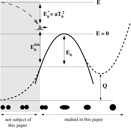
Figure 1: Sketch of the scenario of this paper.

In order to allow for a largely analytic approach the barrier will be supposed to be given by an inverted oscillator. Restricting ourselves to Gaussian distributions in phase space the probability to overcome this barrier is simply given by [9]

$$\Pi(t)=\frac{1}{2}\left[1+\textrm{erf}\left(\frac{q(t)}{\sqrt{2\Sigma_{qq}(t)}}\right)\right]=\frac{1}{2}\,\textrm{erf}\left(-\frac{q(t)}{\sqrt{2\Sigma_{qq}(t)}}\right)$$ (1)

The $q(t)=\langle q\rangle_{t}$ specifies the center of the Gaussian, which moves from left to right and which within this approximation represents the average trajectory. The $\Sigma_{qq}(t)=\langle(q-\langle q\rangle_{t})^{2}\rangle_{t}$ defines the fluctuation of the coordinate. Analogous definitions are used for the kinetic momentum $P$, both for the average trajectory $P(t)$ as well as for the fluctuations $\Sigma_{pp}(t)$ and $\Sigma_{qp}(t)$. Analytical expressions for $q(t)$ and $\Sigma_{qq}(t)$, which may be derived from a Fokker-Planck equation [10], are given in appendix A. Fortunately, when time progresses past a certain ”relaxation time” ($t\gg 1/|z^{-}|$) the probability (1) approaches a finite stationary value:

$$\Pi_{\infty}=\lim_{t\to\infty}\Pi(t)=\frac{1}{2}\,\textrm{erf}\left(-\frac{q_{\infty}}{\sqrt{2\Sigma_{qq}^{\infty}}}\right)\,.$$ (2)

The time dependence of both the coordinate as well as of the fluctuation is determined by the frequencies (see appendix A)

$$z^{\pm}=\frac{1}{2\tau_{\textrm{kin}}}\left(\pm\sqrt{1+\frac{1}{\eta_{b}^{2}}}-1\right)\,.$$ (3)

The $\tau_{\textrm{kin}}$ measures the relaxation of the momentum to the thermal Maxwell distribution and the (dimensionless) parameter $\eta_{b}$ indicates whether the process is under-damped ($\eta_{b}<1$) or over-damped ($\eta_{b}>1$). In terms of the transport coefficients for average motion, inertia $M$, friction $\gamma$ and stiffness $C$, which here is negative $C=-|C|$, these quantities are given by

$$\tau_{\textrm{kin}}=\frac{M}{\gamma}\qquad\text{and}\qquad\eta_{b}=\frac{\gamma}{2\sqrt{|C|M}}=\frac{1}{2}\sqrt{\frac{\tau_{\textrm{coll}}}{\tau_{\textrm{kin}}}}\,.$$ (4)

For strong damping $\eta_{b}\gg 1$, viz $\tau_{\textrm{coll}}\gg\tau_{\textrm{kin}}$, we have

$$z^{+}\longrightarrow\frac{1}{\tau_{\textrm{coll}}}\equiv\frac{|C|}{\gamma}\qquad\text{and}\qquad z^{-}\longrightarrow-\frac{1}{\tau_{\textrm{kin}}}\,.$$ (5)

In this limit only processes are relevant (see (21) and (23)) which take place on the time scale $\tau_{\textrm{coll}}$. Later on we will also need the frequency $\varpi_{b}$ at the barrier,

$$\varpi_{b}=\sqrt{\frac{|C|}{M}}=\frac{1}{\sqrt{\tau_{\textrm{coll}}\tau_{\textrm{kin}}}}\,.$$ (6)

The dynamics of fluctuations is not only controlled by the transport coefficients of average motion but by diffusion coefficients as well. In the classical limit (for collective motion) there is only the one given by the famous Einstein relation $D_{pp}=\gamma T$. In the quantum case and for larger damping there may be another one, $D_{qp}$. Both are to be calculated from the quantal fluctuation-dissipation theorem, if the latter only is generalized to the barrier problem by a suitable analytic continuation [11, 10]. We will address this question in more detail later in sect. 3.2.

Finally, we like to note that, different to the original papers, we want to use dimensionless coordinates and the conjugate momenta of dimension $\hbar$. This means to apply the following canonical replacement

$$q\rightarrow\sqrt{\frac{|C|}{\hbar\varpi_{b}}}\,q\ ,\qquad P\rightarrow\sqrt{\frac{\hbar}{M\varpi_{b}}}\,P\,,$$ (7)

which for the second moments implies

$$\Sigma_{qq}\rightarrow\frac{|C|}{\hbar\varpi_{b}}\,\Sigma_{qq}\ ,\quad\Sigma_{pp}\rightarrow\frac{\hbar}{M\varpi_{b}}\,\Sigma_{pp}\ ,\quad\Sigma_{qp}\rightarrow\Sigma_{qp}\,.$$ (8)

3 Transport coefficients of average motion and diffusion

To distinguish between the coefficients of average motion, $M$, $\gamma$ and $C$, and the diffusion coefficients $D_{\mu\nu}$, the notion transport coefficients will henceforth be reserved for the former. Later on we are going to compare results obtained for microscopic and macroscopic pictures of the dynamics of nucleons inside the nucleus. In the first case this refers to quantal motion of nucleons in a mean field. Within the Gaussian approach quantum effects in collective motion only show up in the diffusion coefficients and, hence, only in the dynamics of the fluctuations. With respect to this property the notion macroscopic limit stands synonymous for the high temperature limit for which the Einstein relation applies.

3.1 Transport coefficients of average motion

Microscopic model:

Concerning the microscopic transport coefficients we use the suggestion made in [8]

$$\tau_{\textrm{kin}} = \frac{1+T^{2}/40}{0.6T^{2}}\ \frac{\hbar}{~{}\textrm{MeV}}$$ (9)

$$\tau_{\textrm{coll}} = \frac{0.6T^{2}}{1+\pi^{2}T^{2}/c_{\textrm{macro}}^{2}}\ \frac{\hbar}{~{}\textrm{MeV}}$$ (10)

(with temperature being measured in MeV). These simple expressions have been developed to resemble the $T$-dependence of the truly microscopic values of $\tau_{\textrm{kin}}(Q,T)$ and $\tau_{\textrm{coll}}(Q,T)$ obtained by application of linear response theory. Using (9) and (10) we calculate the effective damping strength $\eta_{b}(T)$ from (4) and the frequency $\varpi_{b}(T)$ from (6). As may be seen from Fig. 2 the latter may fairly well be approximated by $\varpi_{b}(T)\approx 1~{}\textrm{MeV}/\hbar$. In (10) the $c_{\textrm{macro}}$ is introduced as a parameter to fix the high temperature limit of friction. In more recent times this is claimed to be given not by the wall formula $\gamma_{\textrm{wall}}$ but by about one half of this value, see e.g. [8] and further references given there; we adopt this suggestion. It may be mentioned in passing that the estimates given in (9) and (10) could be extended to include the influence of pairing [8]. The latter diminishes friction at lower temperatures $T\lesssim 0.5~{}\textrm{MeV}$ but its influence is negligible in the range of temperatures used in the present application.

Figure 2: Temperature dependence of relevant ratios of transport coefficients. Critical damping $\eta_{b}=1$ is marked by a dotted line in the bottom right panel. Crosses refer to the microscopic computations of [8] (with pairing included). The solid line represents the fits (9) and (10) to these data. Macroscopic transport coefficients are given by the dashed line [12].

Macroscopic model:

In [4] the friction coefficient is taken from the wall-and-window formula. Like in [8] we will use $\gamma=\gamma_{\textrm{wall}}/2$ here. The macroscopic value of the frequency $\varpi_{b}(T)$ can be calculated from the liquid drop values of stiffness $C_{\textrm{LDM}}(T)$ and inertia $M_{\textrm{LDM}}$; we followed the procedure described in [12]. The ratios $\tau_{\textrm{kin}}(T)$ and $\eta_{b}(T)$ are then fixed by (4).

In Fig. 2 we show a comparison of the temperature dependence of the microscopic and macroscopic transport coefficients used in this paper. It is most important to realize that in the microscopic case collective motion changes from under-damped to over-damped at a temperature $T\approx 2~{}\textrm{MeV}$, whereas in the macroscopic limit collective motion is over-damped ($\eta_{b}>1$) even at very small temperatures. Please have in mind that with increasing $\eta_{b}$ the inertia $M$ becomes less and less important, to drop out entirely for the truly over-damped case. For this reason the estimates given above should be understood to represent those quantities which involve $M$ only for smaller temperatures, up to $T\approx 2\ldots 3~{}\textrm{MeV}$ at best.

3.2 Diffusion coefficients

As mentioned already before, the diffusion coefficients are to be calculated from the fluctuation dissipation theorem. The latter specifies equilibrium fluctuations $\Sigma_{\mu\nu}^{eq}$ to which the dynamical ones turn to at large times (see appendix B or [10]). To evaluate the $\Sigma_{\mu\nu}^{eq,b}$ for a barrier, as represented by an inverted oscillator, requires a suitable analytic continuation involving the change of the stiffness from $|C|$ to $C=-|C|$; details of the procedure may be found in [11, 10]. Accounting for our presently used transformation (8) the relations to the diffusion coefficients become

$$D_{qq}=\Sigma_{qp}^{eq,b}=0\ ,\quad D_{qp}=\hbar\varpi_{b}\,(|\Sigma_{qq}^{eq,b}|-\Sigma_{pp}^{eq,b}/\hbar^{2})\ ,\quad D_{pp}=\tau_{\textrm{kin}}^{-1}\,\Sigma_{pp}^{eq,b}$$ (11)

Please note that the $\Sigma_{qq}^{eq,b}$ of the inverted oscillator is negative.

The application of (11) becomes particularly simple in the high temperature limit. The classic equipartition theorem of Statistical Mechanics implies that one has

$$|\Sigma_{qq}^{eq,b}|=\Sigma_{pp}^{eq,b}/\hbar^{2}=\frac{T}{\hbar\varpi_{b}}\,,\qquad\Sigma_{qp}^{eq,b}=0\qquad\text{for}\qquad T\gg\hbar\varpi_{b}\,.$$ (12)

This is easily recognized considering (8) again. As a consequence, the diffusion coefficients turn to the Einstein relations, which in our case read

$$D_{pp}^{h.T.}=\frac{1}{\tau_{\textrm{kin}}}\,\frac{\hbar T}{\varpi_{b}}=2\hbar\eta_{b}T\,,\qquad D_{qq}^{h.T.}=D_{qp}^{h.T.}=0\,.$$ (13)

For very small damping formulas (12) and (13) keep their form even in the quantum case if only $T$ is replaced by the effective temperature

$$T_{b}^{*}=\frac{\hbar\varpi_{b}}{2}\,\cot\left(\frac{\hbar\varpi_{b}}{2T}\right)\,,$$ (14)

see [13] or [10]. As this requires $\eta_{b}\ll 1$ this limit sometimes is called the zero damping limit. It is seen that friction neither appears in the classical or high temperature limit (12) nor, by definition, in the limit (14) of zero damping.

At lower temperature this is no longer true for the general situation where the size of damping plays an essential role on the temperature dependence of the $\Sigma_{\mu\nu}^{eq,b}$, and hence on the diffusion coefficients. This has already been demonstrated in [11, 10]. In these calculations the transport coefficients of average motion simply appeared as given, constant parameters. As discussed above, they themselves may vary sensitively with $T$. For this reason the calculations of [11] have been repeated using now the specific transport coefficients for average motion described above. The results for $|\Sigma_{qq}^{eq,b}|$ and $\Sigma_{pp}^{eq,b}$ are shown in Fig. 3. It must be said that the calculation of the momentum fluctuations requires regularization of a frequency integral, which comes in through the fluctuation dissipation theorem (29). Also with respect to this problem the same procedure has been applied as in [11] using a Drude regularization with $\omega_{\textrm{D}}\approx 10\varpi$ as the relevant cut-off parameter. As we have $\varpi_{b}(T)\approx 1~{}\textrm{MeV}/\hbar$ (see bottom left panel of Fig. 2) we took the cut-off parameter $\omega_{\textrm{D}}=10~{}\textrm{MeV}/\hbar$ after convincing ourselves that the results are not extremely sensitive to this choice. The variation with $\omega_{\textrm{D}}$ is more pronounced in the case of macroscopic transport coefficients where for $\omega_{\textrm{D}}=5\ldots 20~{}\textrm{MeV}/\hbar$ the momentum fluctuations $\Sigma_{pp}^{eq,b}$ differ from our choice by an additional factor of $0.8\ldots 1.3$ at $T=1~{}\textrm{MeV}$. In the microscopic case the corresponding factor is only $0.8\ldots 1.1$. Paying attention to the fact that the effective damping is quite different in both cases, this is in good agreement with the findings of [11].

In Fig. 3 the $T$-dependence of $\Sigma_{\mu\nu}^{eq,b}$ is exhibited both for the microscopic transport coefficients (left panel) as well as for those in the macroscopic limit (right panel), as described in Sect. 3.1. In each case the fully quantum result is compared with the limits of high temperature (classical) and zero damping.

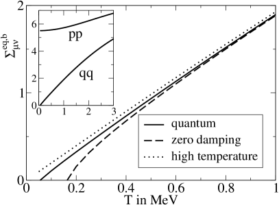
Figure 3: $T$-Dependence of the equilibrium fluctuations of coordinate and momentum calculated in various limits for microscopic (left) and macroscopic transport coefficients (right). The inserts show the behavior at higher temperatures.

It is seen that at very small temperatures the microscopic results are very well represented by the limit of weak damping. For $\Sigma_{pp}^{eq,b}$ the deviations grow faster, a feature which might by related to the fact that the regularization procedure was taken over from [11] without modification. This problem has not been studied any further, simply because the effect of the $\Sigma_{pp}^{eq,b}$ on the transmission probability is weakened by other effects, in particular at larger damping, as will be explained shortly. In any case, the effect seen at small $T$ simply results from the fact that the microscopic damping strength $\eta_{b}$ becomes very small (see lower right part of Fig. 2). Let us note that at large temperatures the microscopic and macroscopic diffusion coefficients approach each other, if normalized to $\hbar\varpi_{b}(T)$, simply because this is so for the transport coefficients of average motion discussed in Sect. 3.1.

4 Numerical results

In the last two subsections it was shown that a proper microscopic treatment of the quantum heat bath has two major effects: (i) the effective damping strength $\eta_{b}$ becomes much smaller than that of macroscopic models and (ii) different to the Einstein relation a second diffusion coefficient $D_{qp}$ shows up. After specifying the initial conditions for our numerical calculations we will examine these effects separately. The effect of quantum diffusion on the formation probabilities (1) and (2) is contrasted with the limits of high temperature (vanishing $D_{qp}$) and zero damping. This will be done both for microscopic as well as macroscopic transport coefficients of average motion.

4.1 Initial conditions

In terms of the barrier height and the initial kinetic energy, expressed by

$$E_{b}=-V_{0}=\frac{\hbar\varpi_{b}}{2}\,q_{0}^{2}\qquad\textrm{and}\qquad E_{0}^{\textrm{kin}}=\frac{\varpi_{b}}{2\hbar}\,P_{0}^{2}$$ (15)

through the initial values of the average coordinate $q_{0}$ and the momentum $P_{0}$, the argument of the error function in (2) turns into

$$\frac{q_{\infty}}{\sqrt{2\Sigma_{qq}^{\infty}}}=\frac{\sqrt{E_{0}^{\textrm{kin}}/\hbar\varpi_{b}}+\sqrt{E_{b}/\hbar\varpi_{b}}\,(z^{-}/\varpi_{b})}{\sqrt{(\Sigma_{pp}(t_{0})-\Sigma_{pp}^{eq,b})/\hbar^{2}+(z^{-}/\varpi_{b})^{2}\,(\Sigma_{qq}(t_{0})-\Sigma_{qq}^{eq,b})-2(z^{-}/\varpi_{b})\,\Sigma_{qp}(t_{0})/\hbar}}\,$$ (16)

see appendix A. A very similar result has been obtained by application of Langevin dynamics to the inverted oscillator [14].

For the barrier height specified in (15) we choose $E_{b}=10~{}\textrm{MeV}$. This is in fair agreement with the typical heights of the inner barriers used in [2]. The initial kinetic energy $E_{0}^{\textrm{kin}}$ and the temperature $T_{0}$ depend on the strength of friction in the approach phase. As in the present paper this problem is not addressed in detail we will simply assume the incident energy $E$ over the barrier top to be strongly dissipated such that a scenario holds as outlined in Fig. 1. As can be seen there, the sum of the initial energy $E$ and the barrier height $E_{b}$ are split into kinetic energy and thermal excitation according to

$$E_{0}^{\textrm{kin}}=R(E+E_{b})\qquad\textrm{and}\qquad E_{0}^{*}=aT_{0}^{2}=(1-R)(E+E_{b}),$$ (17)

with the ratio $0\leq R\leq 1$ to be fixed later. As an estimate for the level density parameter we use the value $a\approx A/10~{}\textrm{MeV}$ where $A$ is the nucleon number of the compound nucleus. In order to keep the computation simple, we assume that temperature stays constant at its initial value $T=T_{0}$ throughout the whole formation process. In Fig. 4 we show the dependence of $T_{0}$ on the energy $E$ for a system of nucleon number $A=224$ and two different assumptions for $R$. In [15] temperatures in the range $T_{0}=0.68\ldots 1.24~{}\textrm{MeV}$ have been studied for a heavier system with $A=298$ nucleons.

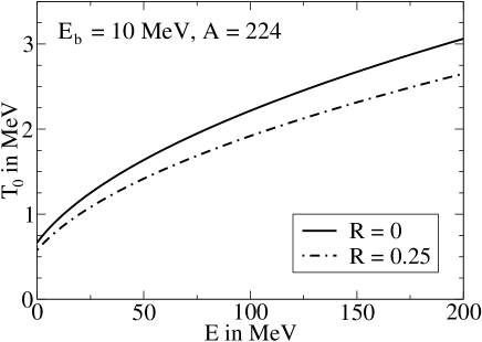
Figure 4: Dependence of the initial temperature on the incident energy.

On the basis of the surface friction model it has been argued that almost no kinetic energy is left after the approach phase, viz at the starting point $q_{0}$ (see for instance Fig. 3 of [3] and Fig. 1b of [4]). In contrast the authors of [5, 6] have suggested damping in the approach phase to be weaker than that of surface friction. In this work we do not want to elaborate on the approach phase but simply incorporate this uncertainty by comparing the case of vanishing initial kinetic energy $E_{0}^{\textrm{kin}}=0$, for which the parameter of (17) becomes $R=0$, with the one of a weaker friction force at large elongations, chosen such that $R=0.25$.

To specify the Gaussian of the initial phase space distribution we need the widths in $q$ and $P$. They shall be parameterized in terms of the $\Sigma_{pp}^{eq,b}$ by introducing two positive numbers $w$ and $W$,

$$\Sigma_{pp}(t_{0})=w\,\Sigma_{pp}^{eq,b}\,,\quad\Sigma_{qq}(t_{0})=W\,\frac{\hbar^{2}}{4w\Sigma_{pp}^{eq,b}}\,,\quad\Sigma_{qp}(t_{0})=0\,.$$ (18)

The $w$ fully determines the momentum fluctuation and the $W$ the one in the coordinate provided the former is given. In case of a strong friction force in the approach phase the $w$ will be close to unity, as then the momentum distribution will be close to Maxwell distribution [10]. The $W$ can be said to define a kind of measure for the overall width of the phase space distribution. Indeed, requiring $W\geq 1$ warrants the uncertainty principle

$$\langle(q-\langle q\rangle_{t_{0}})^{2}\rangle_{t_{0}}\langle(P-\langle P\rangle_{t_{0}})^{2}\rangle_{t_{0}}=\Sigma_{qq}(t_{0})\,\Sigma_{pp}(t_{0})\geq\hbar^{2}/4$$ (19)

to be fulfilled initially. In the limiting case $W=1$ the system starts out of the most narrow distribution still compatible with quantum mechanics. As we want to examine the importance of genuine quantum effects vanishing initial fluctuations $\Sigma_{\mu\nu}(t_{0})\equiv 0$ are prohibited for our studies. One must have in mind, however, that in reality finite fluctuations will have been built up in the approach phase, which may not always be represented by simple Gaussians. In our numerical calculations, the $\Sigma_{pp}^{eq,b}$ which enters the initial conditions (18) is always taken to be the quantum value (see Sect. 3.2), even for studies of the time evolution within high temperature limit.

From the results displayed in Fig. 3 it can be seen that the $\Sigma_{\mu\nu}^{eq,b}$ of the zero damping and high temperature limits may differ considerable from those of the full, quantum results. This difference is particularly large for $\Sigma_{pp}^{eq,b}$ when macroscopic transport coefficients of average motion are used. One might be inclined to believe that at small temperatures this might have a large impact on the formation probabilities $\Pi(t)$ and $\Pi_{\infty}$. However, one must be aware that not only the $\Sigma_{\mu\nu}^{eq,b}$ contribute to the $\Sigma_{qq}^{\infty}$ of the denominator of (16) but the initial fluctuations $\Sigma_{\mu\nu}(t_{0})$ as well. To reveal these effects

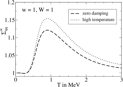
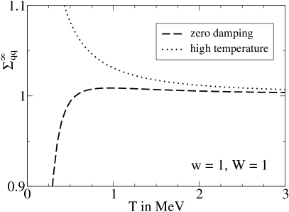
Figure 5: Temperature dependence of the $\Sigma_{qq}^{\infty}$ for the zero damping and high temperature limit, both divided by the general result: left panel for microscopic input, right panel for macroscopic input.

we address in Fig. 5 the $T$-dependence of the $\Sigma_{qq}^{\infty}$. Shown there is the ratio of its values in either the high temperature limit or the zero damping limit to that for the full calculation, for the choice $w=1$ and $W=1$ — for other cases this effect is even smaller. It is seen that the values $\Sigma_{qq}^{\infty}$ obtained in these calculations are quite close to each other. Note, please, that in our studies only temperatures $T\gtrsim 0.6~{}\textrm{MeV}$ are accessible (see Fig. 4). As only the square root of the $\Sigma_{qq}^{\infty}$ appears in (2) one may already deduce here that the three calculations will lead to results which do not differ too much.

4.2 Formation probabilities for microscopic input

We plot the time evolution of the formation probability using the microscopic set of transport coefficients and the fully quantum calculation of the diffusion coefficients in Fig. 6. Results are shown for an incident energy above the barrier of $E=10~{}\textrm{MeV}$ and for vanishing ($R=0$, $E_{0}^{\textrm{kin}}=0$) and finite initial kinetic energy ($R=0.25$, $E_{0}^{\textrm{kin}}=5~{}\textrm{MeV}$). For the parameter $w$, which according to (18) specifies the initial width in the momentum, three different values are used: $w=1/2$ (more narrow than thermal equilibrium), $w=1$ (thermal equilibrium) and $w=2$ (wider than thermal equilibrium). The initial distribution in the coordinate is specified by the two values $W=1$ and $W=3$. In most cases the initial space distribution is almost totally located on the left of the barrier. For the choice $w=1/2$ and $W=3$ a small part of the distribution is on its right already at the beginning. In this case the formation probability $\Pi(t)$ does not start from exactly zero.

In Fig. 6 we show examples corresponding to small effective damping strengths: $\eta_{b}=0.26$ and $\eta_{b}=0.18$ at $T=0.94~{}\textrm{MeV}$ ($R=0$) and $T=0.82~{}\textrm{MeV}$ ($R=0.25$), respectively. As this corresponds to under-damped motion the initial kinetic energy plays an important role on the formation probability. Its stationary value $\Pi_{\infty}$ increases by two orders of magnitude in going from $R=0$ to $R=0.25$. Repeating the same calculations at larger energy $E=50~{}\textrm{MeV}$ reveals additional effects. Enlarging $R$ from $0$ to $0.25$, which is to say for increasing initial kinetic energy and slightly decreasing temperature ($E_{0}^{\textrm{kin}}=0$, $T_{0}=1.6~{}\textrm{MeV}$ in the case $R=0$ and $E_{0}^{\textrm{kin}}=15~{}\textrm{MeV}$, $T_{0}=1.4~{}\textrm{MeV}$ in the case $R=0.25$), the asymptotic value $\Pi_{\infty}$ of $\Pi(t)$ is reached quicker, independently of $w$ and $W$. The influence of the parameters $W$ and $w$ on the value of $\Pi_{\infty}$ is less important than the one of $R$: Varying either $w$ or $W$ mostly implies a change by less than one order of magnitude.

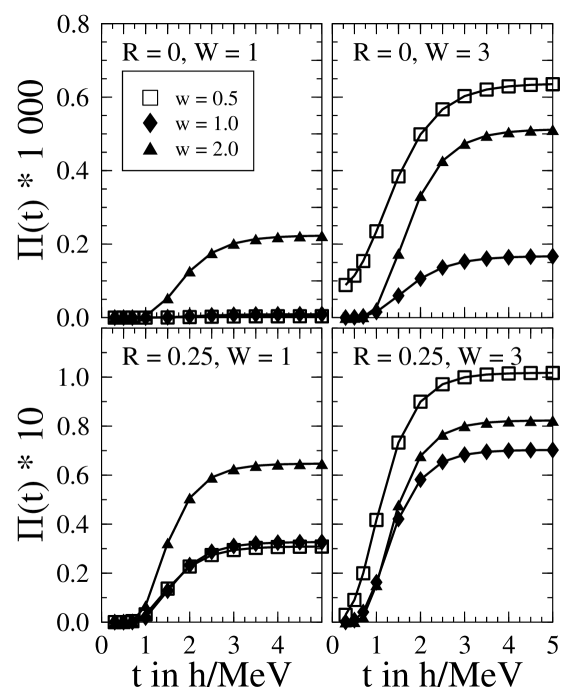
Figure 6: Time evolution of the formation probability $\Pi(t)$ for microscopic transport coefficients and quantum diffusion coefficients, for different choices of the parameters specified in the inserts; the incident energy is $E=10~{}\textrm{MeV}$. Note that the scaling in the upper and lower panels differs by two orders of magnitude. For more details see text.

Next we discuss the energy dependence of the asymptotic value $\Pi_{\infty}$. This is done best by introducing an “effective barrier height” by the following argument: Within the Gaussian approximation the transmission across the barrier is largely governed by the average trajectory. As can be seen from (2) $\Pi_{\infty}$ becomes equal to $1/2$ when the trajectory just hits the top of the barrier at $q_{\infty}=0$. By inspecting the numerator of (16), and recalling from eq.(3) the value of $z^{-}$, one easily recognizes that the trajectories may be classified by their initial kinetic energy $E_{0}^{\textrm{kin}}$ in comparison with the ”effective barrier height” (see also [9, 14, 3])

$$B_{\textrm{eff}}=\left(\sqrt{1+\eta_{b}^{2}}+\eta_{b}\right)^{2}\,E_{b}\geq E_{b}\,.$$ (20)

Trajectories with $E_{0}^{\textrm{kin}}<B_{\textrm{eff}}$ are simply reflected implying the $\Pi_{\infty}$ to be smaller than $1/2$; only those trajectories with $E_{0}^{\textrm{kin}}>B_{\textrm{eff}}$ are able to cross the barrier and the $\Pi_{\infty}$ exceeds $1/2$. Fig. 7 shows the functional dependence of $\Pi_{\infty}$ on the initial kinetic energy scaled to the effective barrier height, for $R=0.25$, $w=1$ and $W=1$ (left) and $W=3$ (right). For several reasons the incident energy is restricted to the interval $E=0\ldots 200~{}\textrm{MeV}$, with a corresponding temperature of $T_{0}=0.6\ldots 2.6~{}\textrm{MeV}$. First of all, at larger temperatures the survival probability becomes too small. Secondly, as mentioned already before, there the motion becomes strongly over-damped, such that formulas which involve the inertia become less and less trustworthy.

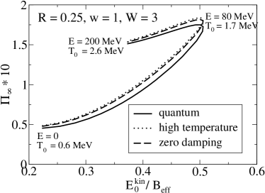
Figure 7: Formation probability $\Pi_{\infty}$ using microscopic transport coefficients as a function of the ratio of the initial kinetic energy (17) to the effective barrier height (20). For $\Sigma_{\mu\nu}^{eq,b}$ we compare the results applying a quantum calculation (comp. [11]) and the limits of high temperature (12) and zero damping (12) with (14). Note that the incident energy changes along the curve: $E=0\ldots 200~{}\textrm{MeV}$. The value $E=10~{}\textrm{MeV}$ corresponds to $E_{0}^{\textrm{kin}}/B_{\textrm{eff}}=0.35$; for details see text.

At small incident energies $E$ (small $T_{0}$), for $\Pi_{\infty}$ a choice of $W=3$ implies a factor of the order $5$ over the case of the most narrow initial distribution which still is compatible with quantum mechanics ($W=1$). This increase of $\Pi_{\infty}$ with $W$ rapidly diminishes with growing $E$. In addition to the full quantum calculation of the diffusion coefficients we show in Fig. 7 the results of the limits of zero damping and high temperature. Both approximations are of about the same quality. For the chosen example quantum effects are seen to be small and become largest at intermediate temperatures $T=0.7\ldots 2~{}\textrm{MeV}$ ($E=5\ldots 120~{}\textrm{MeV}$). Both observations confirm the conjecture made already in connection with Fig. 5.

As a remarkable feature we observe in Fig. 7 a back-bending of the curves representing $\Pi_{\infty}$ at $E_{0}^{\textrm{kin}}/B_{\textrm{eff}}\approx 0.5$. It can be explained as follows: The initial kinetic energy depends on $E$ linearly (see (17)), while the $E$-dependence of the effective barrier height (20) is more complicated and comes in via $\eta_{b}(T_{0}(E))$. As a function of $E$ for $R=0.25$ the ratio $E_{0}^{\textrm{kin}}/B_{\textrm{eff}}$ develops a maximum and a minimum (the latter corresponding to $T_{0}\approx 4~{}\textrm{MeV}$; which is beyond the region considered here). At energies far beyond this range $\Pi_{\infty}$ would approach $1$. The final formation probability also exhibits a shallow maximum near the turning point. This behavior might have some influence on the reasonable choice of incident energies in an experimental setup for heavy ion collisions, because the survival probability decreases with increasing excitation energy $E^{*}$ and therefore smaller $E$ is more favorable for survival.

4.3 Formation probabilities for macroscopic coefficients of average motion

In Fig. 8 we show $\Pi_{\infty}$ as a function of the ratio $E_{0}^{\textrm{kin}}/B_{\textrm{eff}}$ on a logarithmic scale for $E=0\ldots 200~{}\textrm{MeV}$ and $R=0.25$, $w=1$ and $W=3$ using macroscopic transport coefficients now.

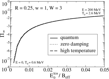
Figure 8: Same quantities as in the right panel of Fig. 7 for macroscopic transport coefficients. The value $E=10~{}\textrm{MeV}$ corresponds to $E_{0}^{\textrm{kin}}/B_{\textrm{eff}}=0.0036$. Note the logarithmic scale.

The back-bending found in Fig. 7 is absent here. Quantum effects of the collective motion qualitatively behave as discussed in Sect. 4.2. Quantitatively at $T=0.8\ldots 1.0~{}\textrm{MeV}$ they are even smaller than in the case of microscopic transport coefficients, comp. Fig. 5. The small differences between the full quantum calculation (of the diffusion coefficients) and the limits of zero damping and high temperature are hardly visible on logarithmic scale.

Due to the fact that for macroscopic transport coefficients collective motion is strongly over-damped ($\eta_{b}=5.9\ldots 4.9$ for $T=0.6\ldots 3~{}\textrm{MeV}$) the effective barrier height (20) is very large now: $B_{\textrm{eff}}=1.4~{}\textrm{GeV}\ldots 980~{}\textrm{MeV}$. Mind that for microscopic transport coefficients the same quantity is in the range $B_{\textrm{eff}}=15\ldots 180~{}\textrm{MeV}$ only (comp. $E_{b}=10~{}\textrm{MeV}$). This leads to ratios $E_{0}^{\textrm{kin}}/B_{\textrm{eff}}$ of about one order of magnitude smaller than for microscopic transport coefficients. This ratio crucially influences the size of the formation probability $\Pi_{\infty}$. Consequently in the case of macroscopic transport coefficients $\Pi_{\infty}$ is several orders of magnitudes smaller than for microscopic ones. This effect increases with decreasing $E$. Compared to this loss of orders of magnitude in $\Pi_{\infty}$ due to the replacement of microscopic by macroscopic transport coefficients, quantum effects in the collective motion due to the type of approximation applied in the calculation of the $\Sigma_{\mu\nu}^{eq,b}$ are of minor importance only.

Figure 9: Same quantities as in Fig. 6 for $E=10~{}\textrm{MeV}$ and macroscopic transport coefficients.

The time dependent behavior of the formation probability $\Pi(t)$ is shown in Fig. 9 for the same initial conditions as for Fig. 6. As mentioned previously, now the effective damping of the collective motion is clearly in the over-damped regime: $\eta_{b}\approx 5.8$ both at $T=0.94~{}\textrm{MeV}$ ($R=0$) and $T=0.82~{}\textrm{MeV}$ ($R=0.25$). The time scale for the rise of $\Pi(t)$ is larger by a factor of the order of $10$, as compared to the microscopic case and completely independent of the initial kinetic energy $E_{0}^{\textrm{kin}}$, viz the initial momentum $P_{0}$. We have checked that different to the case of microscopic transport coefficients this is still true at $E=50~{}\textrm{MeV}$. This is in accord with the fact that for $\eta_{b}\gg 1$ one is in the Smoluchowski limit, for the momentum drops out entirely. For the same reason also the stationary value $\Pi_{\infty}$ is much less sensitive to the initial kinetic energy than in the case of microscopic transport coefficients. Whereas in the microscopic case at $E=10~{}\textrm{MeV}$ we gained two orders of magnitude going from $R=0$ to $R=0.25$ the increase of $\Pi_{\infty}$ now is invisibly small. Using the large energy $E=50~{}\textrm{MeV}$ the corresponding increase is at most by a factor of $2$ whereas in the microscopic case we gain two orders of magnitude, too.

5 Summary and conclusion

Concentrating on the formation probability we have been able to demonstrate the importance of microscopic transport coefficients of average motion. As compared to those of macroscopic pictures like that of the liquid drop model and wall friction, they may increase the formation probabilities by a few orders of magnitude. This is especially important at smaller temperatures where the dynamics of nucleons in a mean field is dominated by quantum effects and where ”collisional damping” is suppressed [10]. For collective motion this implies a moderate to weak damping.

In contrast to this, quantum effects in collective motion would become relevant only at even smaller temperatures. In a sense, this is in accord with the findings in [7] for nuclear fission. Since at small $T$ friction is suppressed quantal diffusion coefficients may be estimated within the so called ”zero friction limit”. This feature applies only for the microscopic picture of nucleonic dynamics. In fact, in this paper it was the first time that microscopic transport coefficients have been used when calculating the diffusion coefficients for collective dynamics through the quantal fluctuation dissipation theorem. Because of the delicate temperature dependence of the transport coefficients this procedure is vital to get decent answers.

Another issue of our studies was to examine the relevance of the initial conditions for the phase space distribution. Whenever the whole process of fusion is split into parts where the entrance phase is treated differently from the formation of the compound nucleus uncertainties for the initial conditions of the formation process are more or less inherent. Evidently, such a situation would only be given if the intermediate step would correspond to a kind of quasi-equilibrium; in remote sence in analogy to N. Bohr’s hypothesis of a two step process. Indeed, as we have seen, for a more quantitative calculation of the reaction cross section it will be inevitable to follow the whole process, entrance phase plus formation. It is only then that the ”initial conditions” for the latter can be known better. Unfortunately, however, it is only fair to say that a decent microscopic picture for the first stage is still lacking.

Acknowledgments:

The authors would like to thank F.A. Ivanyuk for critical and fruitful discussions and D. Boilley for helpful comments.

Appendix A Average coordinate and fluctuations

Using dimensionless coordinates and the conjugate momenta (7) the solution of the equations of motion for the average trajectory reads in the case of the inverted oscillator [10]:

$$q(t) = \frac{1}{2{\cal E}_{b}}\,(\varpi_{b}P_{0}/\hbar-q_{0}z^{-})\,\exp(z^{+}(t-t_{0}))$$ (21)

$$+ \frac{1}{2{\cal E}_{b}}\,(-\varpi_{b}P_{0}/\hbar+q_{0}z^{+})\,\exp(z^{-}(t-t_{0}))$$

Here $q_{0}=q(t_{0})$ and $P_{0}=P(t_{0})$ are the initial coordinate and momentum respectively and the frequencies $z^{\pm}$ are defined in (3); ${\cal E}_{b}=(2\tau_{\textrm{kin}})^{-1}\sqrt{1+\eta_{b}^{-2}}$. For long times $t\gg 1/|z^{-}|$ (21) reduces to

$$q(t)\sim\frac{1}{2{\cal E}_{b}}\,(\varpi_{b}P_{0}/\hbar-q_{0}z^{-})\,\exp(z^{+}(t-t_{0}))\,.$$ (22)

In dimensionless coordinates the fluctuations of the coordinate of the inverted oscillator read (comp. [10]):

$$\Sigma_{qq}(t) = A_{1}\,\frac{\varpi_{b}^{2}}{\hbar z^{-}}\,\exp(2z^{-}(t-t_{0}))+A_{2}\,\frac{\varpi_{b}^{2}}{\hbar z^{+}}\,\exp(2z^{+}(t-t_{0}))$$ (23)

$$+A_{3}\,\frac{\varpi_{b}}{\hbar\eta_{b}}\,\exp((z^{-}+z^{+})(t-t_{0}))+\Sigma_{qq}^{eq,b}$$

Here the abbreviations

$$A_{1} = \frac{z^{-}}{(z^{+}-z^{-})^{2}}\,\left[-2\,\frac{z^{+}}{\varpi_{b}}\,c+\left(\frac{z^{+}}{\varpi_{b}}\right)^{2}\,b+a\right]$$ (24)

$$A_{2} = \frac{z^{+}}{(z^{+}-z^{-})^{2}}\,\left[-2\,\frac{z^{-}}{\varpi_{b}}\,c+\left(\frac{z^{-}}{\varpi_{b}}\right)^{2}\,b+a\right]$$ (25)

$$A_{3} = \frac{z^{+}+z^{-}}{(z^{+}-z^{-})^{2}}\,\left[-\frac{z^{-}+z^{+}}{\varpi_{b}}\,c+\frac{z^{-}z^{+}}{\varpi_{b}^{2}}\,b+a\right]$$ (26)

and

$$\left(\begin{array}[]{c}a\\ b\\ c\end{array}\right)=\left(\begin{array}[]{c}(\Sigma_{pp}(t_{0})-\Sigma_{pp}^{eq,b})/\hbar\\ (\Sigma_{qq}(t_{0})-\Sigma_{qq}^{eq,b})\hbar\\ \Sigma_{qp}(t_{0})\end{array}\right)$$ (27)

have been applied (note the small differences in the definitions compared to [10] that make the expressions more symmetric). The long time limit of (23) reads:

$$\Sigma_{qq}(t)\sim A_{2}\,\frac{\varpi_{b}^{2}}{\hbar z^{+}}\,\exp(2z^{+}(t-t_{0}))$$ (28)

Appendix B Implications of the fluctuation dissipation theorem

For a stable system the equilibrium fluctuations of some quantity $A_{\mu}$ can be calculated from the quantal fluctuation dissipation theorem in its normal form:

$$\Sigma_{\mu\nu}=\hbar\int\frac{d\omega}{2\pi}\,\coth\frac{\hbar\omega}{2T}\,\chi_{\mu\nu}^{\prime\prime}(\omega)$$ (29)

Here, $\chi_{\mu\nu}^{\prime\prime}$ is the dissipative part of the response function that describes the variation of the average of $A_{\mu}$ to a small change of the “external field” $a_{\nu}$ which couples to the system through an interaction $\delta H=\sum_{\nu}A_{\nu}a_{\nu}(t)$. For the present case, the average $\langle A_{\mu}\rangle$ either refers to the coordinate $q$ or the momentum $p$.

Unstable modes, which appear in the barrier region, may be treated by analytic continuation [11], changing a positive stiffness into a negative one. In this way the stationary fluctuations of the damped inverted oscillator (of frequency $\varpi_{b}$ and effective damping $\eta_{b}$) become:

$$\Sigma_{qq}^{eq,b} = -\frac{T}{\hbar\varpi_{b}}\left(1-\frac{\hbar\varpi_{b}^{2}}{\pi T}\times\right.$$ (30)

$$\left.\sum_{j=1}^{3}\frac{\varpi_{D}-\textrm{i}\omega^{(j)}}{(\omega^{(j)}-\omega^{(j+1)})(\omega^{(j)}-\omega^{(j+2)})}\Psi\left(1+\textrm{i}\,\frac{\hbar\omega^{(j)}}{2\pi T}\right)\right)$$

$$\Sigma_{pp}^{eq,b} = \hbar^{2}\left(|\Sigma_{qq}^{eq,b}|+\frac{\varpi_{D}}{\pi\tau_{\textrm{kin}}\varpi_{b}}\times\right.$$ (31)

$$\left.\sum_{j=1}^{3}\frac{-\textrm{i}\omega^{(j)}}{(\omega^{(j)}-\omega^{(j+1)})(\omega^{(j)}-\omega^{(j+2)})}\Psi\left(1+\textrm{i}\,\frac{\hbar\omega^{(j)}}{2\pi T}\right)\right)$$

$$\Sigma_{qp}^{eq,b} = 0$$ (32)

Here $\varpi_{D}\gg\varpi_{b}$ is the so called Drude cut-off frequency necessary to regularize the $\omega$-integral in (29) in the case of $\Sigma_{pp}^{eq,b}$. We have put $\varpi_{D}=10~{}\textrm{MeV}/\hbar$ in this paper and the frequencies $\omega^{(j)}$ are the solutions of the equation

$$-\varpi_{b}^{2}-\textrm{i}\omega\left(-\frac{\varpi_{b}^{2}}{\varpi_{D}}+\frac{1}{\tau_{\textrm{kin}}}\right)-\omega^{2}+\textrm{i}\,\frac{\omega^{3}}{\varpi_{D}}=0$$ (33)

(periodicity is assumed: $\omega^{(j+3)}\equiv\omega^{(j)}$).

References

- [1] N. Antonenko, E. Cherepanov, A. Nasirov, V. Permjakov, and V. Volkov, Phys. Rev. C 51, 2635 (1995); G. Adamian, N. Antonenko, W. Scheid, and V. Volkov, Nucl. Phys. A 633, 409 (1998).
- [2] V. Y. Denisov and S. Hofmann, Phys. Rev. C 61, 034606 (2000).
- [3] Y. Abe, Eur. Phys. J. A 13, 143 (2002).
- [4] C. Shen, G. Kosenko, and Y. Abe, Phys. Rev. C 66, 061602 (2002).
- [5] G. Kosenko, C. Shen and Y. Abe, J. Nucl. Radiochem. Sci. 3, 19 (2002).
- [6] Y. Aritomo and M. Ohta, Phys. Atom. Nucl. 6, 1 (2003).
- [7] H. Hofmann and F. A. Ivanyuk, Phys. Rev. Lett. 82, 4603 (1999).
- [8] H. Hofmann, F. A. Ivanyuk, C. Rummel, and S. Yamaji, Phys. Rev. C 64, 054316 (2001).
- [9] H. Hofmann and P. Siemens, Phys. Lett. B 58, 417 (1975).
- [10] H. Hofmann, Phys. Rep. 284 (4&5), 137 (1997).
- [11] H. Hofmann and D. Kiderlen, Int. J. Mod. Phys. E 7, 243 (1998).
- [12] F. A. Ivanyuk, H. Hofmann, V. Pashkevich, and S. Yamaji, Phys. Rev. C 55, 1730 (1997).
- [13] K. Pomorski and H. Hofmann, J. Physique 42, 381 (1981).
- [14] Y. Abe, D. Boilley, B. G. Giraud, and T. Wada, Phys. Rev. E 61, 1125 (2000).
- [15] Y. Aritomo, T. Wada, M. Ohta, and Y. Abe, Phys. Rev. C 59, 796 (1999).