Rescattering and finite formation time effects in inclusive and exclusive electro-disintegration of nuclei within a relativistic approach: 1. The deuteron

Abstract

The rescattering contribution to the inclusive and exclusive deuteron electro-disintegration at the values of the Bjorken scaling variable $x=1$, as well as in the so called cumulative region ($x>1$) is calculated within a relativistic approach based on the Feynman diagram formalism taking also into account colour transparency effects by the inclusion of the finite formation time (FFT) of the ejected nucleon via the introduction of the dependence of the scattering amplitude of the ejectile upon its virtuality. In the cumulative region the FFT effects which result from the real part of the ejectile propagator are taken into account. It is found that the relative weight of the rescattering steadily grows with $x$ becoming of the order of unity at $x>1.4\div 1.5$. At such values of $x$ the finite formation time effects become fairly visible, which may serve for their study at relatively small value of the four-momentum transfer $Q^{2}$. The relativistic rescattering contribution is compared with the Glauber rescattering, which is shown to be not valid in the cumulative region starting from $x>1.4$.

I Introduction

Quasi-elastic inclusive and exclusive high energy electron scattering off nuclei of the type $A(e,e^{\prime})X$, $A(e,e^{\prime}h)X$, etc, where $h$ denotes a hadron, represent powerful tools to investigate both the properties of hadronic matter, as well as basic QCD predictions, provided one is able to evaluate the effects of the Final State Interaction (FSI) of the lepto-produced hadrons. As a matter of fact, the possibilities to get information on basic properties of bound hadrons, such as, for example their momentum and energy distributions, crucially depend upon the ability to estimate to which extent FSI effects destroy the direct link between the measured cross section and the hadronic properties before interaction with the probe, so the main aim is to minimize the effects of FSI. At the same time, the necessity for an accurate treatment of FSI, stems from the QCD prediction that at large $Q^{2}$ FSI should vanish because of Color Transparency (CT) zamo - brodsky (for recent reviews on the subject, see e.g. color ,niko ), according to which the rescattering amplitudes of the hit nucleon (the ejectile) corresponding to various excited states interfere destructively. This is equivalent to the Gribov inelastic corrections gribov to the Glauber multiple scattering approximation. Thus the experimental investigation of CT is thought to be the detection of possible differences between experimental data and predictions of standard Glauber multiple scattering calculations of FSI. While there is a vast consensus on the qualitative features of the effect, the quantitative aspects are still under debate and many details in the theoretical formulation of the problem are not unique. Most problems arise for the following reason: whereas the Glauber approach is a workable and reliable approximation to the scattering of hadrons off nuclei, problems may arise when one is treating the rescattering of a hadron produced in the medium. Therefore one faces both the problem of calculating the usual rescattering of the produced hadron and the introduction of CT effects. The standard approach to CT is formulated in terms of a multi-channel problem, the vanishing of FSI taking place via the cancellation between contributions from channels with various excitations of the nucleon. This cancellation is expected to become fully operative in a high energy regime, when, at least, several nucleon states are excited. Where precisely such a regime is located is not yet quite clear. Present evidence from experimental exp and theoretical comparison investigations of quasi-elastic $A(e,e^{\prime}p)X$ reactions seems to indicate that CT effects are not visible up to $Q^{2}$ of the order 20 (GeV/c)². The treatment of CT within the multi-channel Glauber approach inevitably involves many poorly known quantities, related both to the structure of the tower of excited nucleon states and to diagonal and non-diagonal amplitudes for their rescattering. It also usually leads to rather heavy expressions for numerical evaluation. This makes the predictions of various approaches not unique and sometimes even conflicting. A formally different, though physically equivalent approach for the treatment of FSI in lepto-production processes has been recently developed BCT , based upon a direct evaluation of Feynman diagrams and assuming an explicit dependence of the nucleon-nucleon scattering amplitude on the virtuality of the ejectile; by this way one introduces a finite formation time (FFT) for the produced hadronic state to become a physical hadron. In this approach, which, for a single rescattering is equivalent to the CT in a two-channel approach, FSI vanish because with increasing $Q^{2}$ the virtuality also increases and the amplitudes diminish. The approach has been applied to the inclusive process $A(e,e^{\prime})X$ at the value of the Bjorken scaling variable $x=Q^{2}/(2M\nu)\simeq 1$. In this paper we generalize the approach to $x>1$ and to exclusive processes $A(e,e^{\prime}p)B$ for which a large wealth of papers, aimed at investigating CT effects, already exists at $x=1$, where the energy in the final state is sufficiently high to produce physical nucleon resonant states. The aim of this paper is to investigate CT (FFT) effects also at $x>1$, i.e. in the so called cumulative region. We will present here the results for the deuteron, leaving a discussion for complex nuclei for subsequent paper. The cumulative region has not been much investigated in the past on the basis of the conjecture that the influence of CT should be much smaller than at $x\simeq 1$, since the available final state energy may be insufficient to produce those excited states of the hit nucleon, whose contribution is to cancel the one coming from the lowest scattering states. Nonetheless the importance of the investigation of CT effects in the cumulative region has been stressed Ref. kope , where it has been shown that, due to the different role played by the Fermi motion, CT effects should strongly depend upon the value of $x$, so that such a dependence should represent a possible signature of CT. Such a conclusion, which is certainly well-grounded, was however based on the Glauber picture for the rescattering, in which the hit nucleon which rescatters with the other $A-1$ particles (the ejectile) is taken on its mass shell during rescattering. In reality the ejectile may also rescatter in a virtual state, below the energy necessary for it physical excitation. Thus only a part of the rescattering contribution vanishes at low energies, namely that coming from the imaginary part of the ejectile propagator, whereas the one coming from the real part does not vanish and may feel the influence of excited ejectile states created virtually. Obviously this effect can be felt only if one goes beyond the Glauber approximation for the rescattering.

We have investigated this problem by a direct calculation of rescattering contribution in the cumulative region starting from the relevant Feynman diagrams. It should be stressed here that a rigorous relativistic description in the cumulative region encounters difficulties of principle already at the level of the impulse approximation; these difficulties are mainly related to the treatment of the unknown electromagnetic form-factors for an off-mass-shell nucleon, so that the calculation of the rescattering and FFT contribution with relativistic spins is out of the question with the present calculational possibilities. One has therefore to recur to some approximations to make calculations viable. In our approach, we calculate the amplitudes in a relativistic manner treating, however, the deuteron and the nucleons as spinless particles; the approximation is cured by introducing an effective electromagnetic form-factor of the nucleon suitably chosen to take into account the magnetic moments. We will demonstrate that at the level of the IA such a procedure provides results in a very good agreement with calculations performed within a full treatment of spin CKT , which makes us confident that the rescattering and FFT contributions calculated with these effective form-factors represents a meaningful approximation. Since we are assuming a quasi-elastic mechanism of $\gamma^{*}$ interaction with a bound nucleon, thanks to the high cumulativity $(x>1)$ of the process, the invariant mass of the final hadronic state does not strongly differ from the nucleon mass, so that one can simply use elastic rescattering amplitudes for the rescattering contribution. Most important, in this region the pole contributions responsible for the FFT, do not contribute at all and all the FFT effect originates from the non-Glauber contribution due to the real part of the ejectile propagator. So we shall be able to study directly the importance of this effect neglected in previous treatments of CT effects. Our results show that the relative weight of the rescattering contribution steadily grows with $x>1$ reaching 50% already at $x=1.5$. The CT or FFT effects, indeed very small at $x<1.3\div 1.4$, become quite pronounced at larger $x$. So, contrary to usual expectations, the study of rescattering on the deuteron allows to see these effects quite clearly. As already mentioned, our numerical results are obtained in a relativistic approach; the approach based on the Glauber picture with relativistic kinematics exhibits no FFT effects, as predicted in kope , but fails to reproduce the rescattering contribution above $x\sim 1.2$.

Our paper is organized as follows: in Section 2 the general formalism for treating inclusive and quasi-exclusive cross sections will be presented; the Impulse Approximation will be described in Section 3 whereas the rescattering and FFT effects will be treated in Section 4. The numerical results are given in Section 5, Conclusions are drawn in Section 6. In Appendices A and B, several details concerning the numerical calculations are given.

II Kinematics, structure functions and cross-sections

In the relativistic domain the nucleon struck by the virtual photon may be excited to states with higher masses. At very high energies this leads to the standard picture of Deep Inelastic Scattering (DIS) in terms of quarks and gluons. We are interested in this Paper in the quasi-elastic (q.e.) scattering, when the final produced hadronic state is just a nucleon. To achieve this and stay within the description in terms of nucleons, we choose the kinematical region of deep enough cumulativity, $x$ close to 2 , where the total mass of the final hadronic systems remains low, below the threshold for the formation of excited nucleon states.

Thus the process we are investigating is as follows

$$e+d\to e+p+n$$ (1)

and in our calculations we simply use elastic rescattering amplitudes for the rescattering inside the deuteron.

We will consider both the inclusive process $d(e,e^{\prime})np$, when only the scattered electron is detected in the final state, as well as the exclusive process $d(e,e^{\prime}p)n$, when also the proton is detected in coincidence with the scattered electron.

The main kinematical quantities involved in the process will be denoted as follows:

1. $M$ and $m$ denote the deuteron and nucleon masses, respectively;

2. $k\equiv(E,{\bf k})$ and $k^{\prime}\equiv(E^{\prime},{\bf k}^{\prime})$ are the four-momenta of the incoming and scattered electrons, respectively;

3. $q\equiv(q_{0},{\bf q})$ is the photon momentum, $Q^{2}=-q^{2}=4EE^{\prime}sin^{2}{{\frac{\theta}{2}}}$ the four-momentum transfer, $\nu=qp/m$, and $\theta$ and $\phi$ the electron scattering angles in the lab system, where $\nu=E-E^{\prime}$;

4. the quantity

   $$x=\frac{Q^{2}}{2qp}$$ (2)

   is the Bjorken scaling variable defined with respect to the $\gamma^{*}+N$ scattering, so that

   $$0\leq x\leq 2$$ (3)

   The region $x>1$ is called cumulative;

5. the deuteron momentum is denoted by $P=2p$; $k_{1(2)}$ are the momenta of nucleon $1(2)$ before interaction with ${\gamma^{*}}$ and $p_{1(2)}$ are the momenta of nucleon $1(2)$ in the final state;

6. we use light-cone coordinates, $a_{+}$, $a_{-}$ defined in the usual way viz. $a_{+(-)}=(a_{0}\pm a_{z})/\sqrt{2}$. The independent variables for each nucleon $i=1,2$ are its transverse momentum component and the carried fraction of the momentum $p_{+}$ (scaling variable): $k_{\perp,i}$ and $x_{i}$ before the interaction and $p_{\perp,i}$ and $\zeta_{i}$ in the final state. Obviously $x_{1}+x_{2}=1$ and $\zeta_{1}+\zeta_{2}=2+\xi$ where $\xi$ is the scaling variable of the photon (see Eq. (13) below).

7. in the following we will also need the definition of the nucleon virtuality $v$ which is

   $$v=m^{2}-k_{1}^{2}$$ (4)

   for the nucleon before $\gamma^{*}$ absorption, and

   $$v^{\prime}=m^{2}-(k_{1}+q)^{2}$$ (5)

   for the nucleon after absorption.

Since, as it will be shown later on, the exclusive cross section will be obtained by a proper procedure from the structure functions appearing in the definition of the inclusive cross section, some general relations concerning kinematics and structure functions relevant for both inclusive and exclusive processes will be derived, starting from the definition of the inclusive cross section. In terms of the standard structure functions $F_{1(2)}(x,Q^{2})$, one has

$$\sigma_{incl}\equiv\frac{d\sigma}{dE^{\prime}d\Omega^{\prime}}=\sigma_{Mott}\frac{1}{4\pi M}\left(\frac{M^{2}}{qP}F_{2}(x,Q^{2})+2\tan^{2}\frac{\theta}{2}F_{1}(x,Q^{2})\right)$$ (6)

where

$$\sigma_{Mott}=\left({\alpha\,\,\cos{\theta\over 2}\over 2{E}\sin^{2}{\theta\over 2}}\right)^{2}$$ (7)

is the Mott cross section. In our normalization the inclusive structure functions are related to the imaginary part of the forward amplitude for the elastic $\gamma^{*}+d$ scattering (hadronic tensor) as

$$W_{\mu\nu}=\left(-g_{\mu\nu}+\frac{q_{\mu}q_{\nu}}{q^{2}}\right)F_{1}(x,Q^{2})+\frac{1}{qP}\left(P_{\mu}-q_{\mu}\frac{qP}{q^{2}}\right)\left(P_{\nu}-q_{\nu}\frac{qP}{q^{2}}\right)F_{2}(x,Q^{2})$$ (8)

and the standard way to find the structure functions from $W_{\mu\nu}$ is to choose a coordinate system ( the theoretical system) in which $q_{+}=q_{y}=p_{\perp}=0$. Labeling the components of vectors and tensors in this system with bars, one finds

$$F_{1}(x,Q^{2})=\bar{W}_{yy},\ \ F_{2}(x,Q^{2})=\frac{Q^{2}}{4xp_{+}^{2}}\bar{W}_{++}$$ (9)

We take the deuteron at rest, ${\bf p}=0$, but in order to simplify the calculations of the rescattering contribution, we choose a system in which $q_{\perp}=0$ ( the lab frame for the system $\gamma^{*}+d$), instead of $q_{+}=q_{y}=0$. These two systems are related by a rotation in the $xz$ plane by the angle

$$\phi_{0}=\arctan\frac{xM}{Q}$$ (10)

For any vector $k$ we find, in particular

$$\bar{k}_{+}=c_{+}k_{+}+c_{-}k_{-}+c_{x}k_{x},\ \ {\bar{k}}_{y}=k_{y},$$

$$c_{+}=\frac{1}{2}(1+\cos\phi_{0}),\ \ c_{-}=\frac{1}{2}(1-\cos\phi_{0}),\ \ c_{x}=\frac{1}{\sqrt{2}}\sin\phi_{0}$$ (11)

These relations will serve to transform to the lab system the structure functions $F_{1,2}$ resulting from our calculation in the chosen system.

In the system $q_{\perp}=0$ the longitudinal components of $q$ are

$$q_{0}=\frac{Q^{2}}{xM},\ \ q_{z}=-Q\sqrt{\frac{Q^{2}}{x^{2}M^{2}}+1}$$ (12)

wherefrom we find the light-cone components

$$q_{\pm}=\frac{Q^{2}}{xM\sqrt{2}}\left(1+\sqrt{1\mp\frac{x^{2}M^{2}}{Q^{2}}}\right),\ \ q_{+}=\xi p_{+}$$ (13)

Evidently $\xi$ is negative and tends to $-x$ when $Q^{2}\to\infty$. Note that in our system the photon moves along the opposite direction of the $z$-axis.

Using the expression (13) for the light-cone components of $q$ one obtains for the virtualities given by Eqs. (4, 5)

$$v=2\frac{m^{2}+k_{1\perp}^{2}}{x_{2}}-\frac{1}{2}x_{1}M^{2}$$ (14)

and

$$v^{\prime}=Q^{2}\left(1-\frac{2-x_{2}}{x}\right)+m_{2\perp}^{2}\frac{2+\xi}{x_{2}}-\frac{1}{2}M^{2}\left(2-x_{2}+\frac{1}{2}\xi x_{2}\right)$$ (15)

The total c.m. energy squared for the reaction $\gamma^{*}-d$ is

$$s=(2p+q)^{2}=Q^{2}\frac{2-x}{x}+M^{2}$$ (16)

As already mentioned, we shall choose the kinematical domain where formation of excited two-nucleon states is impossible or, at least, strongly suppressed, so that the reaction $\gamma^{*}+d$ is essentially binary, i.e. :

$$\gamma^{*}(q)+d(P)\to N(p_{1})+N(p_{2})$$ (17)

As a result, the scaling variables and transverse momenta of the final nucleons are constrained by energy conservation

$$s=(m^{2}+p_{1\perp}^{2})\left(2+\frac{\zeta_{1}}{\zeta_{2}}+\frac{\zeta_{2}}{\zeta_{1}}\right)$$ (18)

The kinematical limits on $\zeta_{1,2}$ are determined by the condition that $p_{1\perp}^{2}>0$ in (18), which leads to

$$\frac{1}{2}(2+\xi)\left(1-\sqrt{1-\frac{4m^{2}}{s}}\right)\leq\zeta_{1,2}\leq\frac{1}{2}(2+\xi)\left(1+\sqrt{1-\frac{4m^{2}}{s}}\right)$$ (19)

At the limiting values of $\zeta_{1,2}$, we have  $p_{1\perp}=0$.

The energy and $z$-component of the momentum of the active nucleon after absorption of the photon (the fast nucleon or ejectile) are given by

$$p_{10}=\frac{1}{4}M\left(\zeta_{1}+\frac{4(m^{2}+p_{1\perp}^{2})}{\zeta_{1}M^{2}}\right),\ \ p_{1z}=\frac{1}{4}M\left(\zeta_{1}-\frac{4(m^{2}+p_{1\perp}^{2})}{\zeta_{1}M^{2}}\right)$$ (20)

They get large if either $p_{1\perp}$ is large or $\zeta_{1}$ is small.

To finish this kinematical excursion, note that the scaling variable of the active nucleon before absorption of the photon is given by

$$x_{1}=\zeta_{1}-\xi$$ (21)

which is different from the scaling variable of the ejectile nucleon and greater than it (since $\xi$ is negative). In the high-energy limit $Q^{2}\to\infty$ $\xi=-x$ and Eq. (21) transforms into $x_{1}=\zeta_{1}+x$. Also Eq. (15) goes into

$$v^{\prime}_{Q^{2}\to\infty}\simeq Q^{2}\left(1-\frac{x_{1}}{x}\right)$$ (22)

from which the standard relation $x^{\prime}=x$ follows if the ejectile lies on the mass-shell.

III The Impulse approximation

III.1 The inclusive cross section

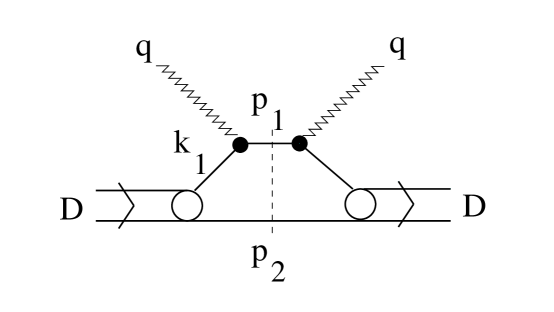
Figure 1: The forward $\gamma^{*}$- d scattering amplitude corresponding to the Plane Wave Impulse Approximation.

In the impulse approximation, depicted in Fig. 1, the imaginary part of the forward $\gamma^{*}+d$ scattering amplitude is given by

$$W_{\mu\nu}=4\gamma^{2}(Q^{2})\int dVK_{\mu}K_{\nu}G^{2}(v)$$ (23)

where $\gamma$ is the effective electromagnetic form-factor of the (scalar) nucleon depending only upon $Q^{2}$, since we assume that its dependence on the virtuality of the proton before the interaction is effectively taken into account by the deuteron wave function. The invariant phase volume element is

$$dV=\frac{d^{2}p_{1\perp}d\zeta_{1}}{16\pi^{2}\zeta_{1}}\delta(m^{2}-k_{2}^{2})=\frac{d\zeta_{1}d\phi}{16\pi^{2}(2+\xi)}$$ (24)

where notations have been used which will be convenient for the following study of rescattering effects, namely $k_{2}=p_{2}=q+2p-p_{1}$ denotes the momentum of the recoil neutron, and, accordingly, $x_{2}\equiv\zeta_{2}$; note, moreover, that $k_{2\perp}=-k_{1\perp}=-p_{1\perp}$.

In Eq.(23), the function $G(v)$ is the relativistic deuteron wave function with the spectator on the mass shell:

$$G(v)=\frac{\Gamma(p,k_{1})}{m^{2}-k_{1}^{2}}$$ (25)

where $\Gamma(p,k_{1})$ is the vertex function describing the virtual decay of the deuteron into two nucleons, and $v$ denotes the virtuality of the active nucleon before interaction, defined previously (Eq. (4))

In Eq. (23) the four-momentum $K$ has to be chosen to guarantee conservation of the electric current from the condition $qK=0$. In our light-cone kinematics we find

$$K=k_{1}+yq$$ (26)

with

$$y=\frac{qk_{1}}{Q^{2}}=\frac{1}{Q^{2}}\left(Q^{2}\frac{x_{1}}{2x}+\frac{1}{8}x_{2}\xi M^{2}-\frac{\xi}{2x_{2}}m_{2\perp}^{2}\right)$$ (27)

Two relevant quantities which we need for the evaluation of the scattering amplitude $W_{\mu\nu}$ are:(i) the virtuality of the off-shell nucleon after interaction defined by Eq. (15), and (ii) the components of $W$ in the theoretical system; using (11) we get

$$\bar{W}_{++}=4\gamma^{2}\int dVG^{2}(v)\Big{[}c_{+}K_{+}+c_{-}K_{-}+c_{x}K_{x}\Big{]}^{2}$$ (28)

$$\bar{W}_{yy}=W_{yy}=4\gamma^{2}\int dVG^{2}(v)K_{y}^{2}$$ (29)

In the lab system neither the longitudinal components of $K$ nor the virtuality $v$ depend on the azimuthal angle $\phi$. The $x$ and $y$-components of $K$ are $|p_{1}|\cos\phi$ and $|p_{1}|\sin\phi$ . So the azimuthal integrations in (28) and (29) are trivial: they give an overall factor $2\pi$ and an additional 1/2 for the square of transverse components. We finally obtain

$$\sigma_{incl}^{IA}=\frac{\sigma_{Mott}}{4\pi M}\int d\zeta_{1}I(|{\bf p}_{2}|,x,Q^{2})$$ (30)

where

$$I(|{\bf p}_{2}|,x,Q^{2},\theta)=\frac{\gamma^{2}}{2\pi(2+\xi)}G^{2}(v)\Big{[}2(c_{+}K_{+}+c_{-}K_{-})^{2}+p_{2\perp}^{2}\left(c_{x}^{2}+\tan^{2}(\theta/2)\right)\Big{]}$$ (31)

Here we have taken into account that due to energy conservation, at fixed $\zeta_{1}$ (or $\zeta_{2}=2+\xi-\zeta_{1}$) both the longitudinal and transverse components of the observed and recoiled nucleons become fixed. In fact $p_{1\perp}^{2}$ is determined by $\zeta_{1}$ via Eq. (18). With $p_{1\perp}^{2}$ known the longitudinal component $p_{1z}$ is found using the second of Eqs. (20).

Note that $x\sim 1$ and/or small scattering angles $\theta$ the integrand $I$ is practically independent of $\theta$ and related only to the internal structure of the deuteron.

In 30 one is left only with one non-trivial integration over $\zeta_{1}$, which has to be done numerically. This is a big advantage of the chosen system: in the theoretical system $v$ results $\phi$-dependent, so that one encounters two numerical integrations. For the impulse approximation this is still viable, but passing to rescattering the number of non-trivial integrations rises to five, which makes the theoretical system impractical.

III.2 The exclusive cross section

We will consider now the exclusive process (1) when the the fast nucleon with momentum $p_{1}=\{\zeta_{1},p_{1\perp}\}$ is observed in coincidence with the scattered electron. As is well known, the hadronic tensor for the exclusive $d(e,e^{\prime}p)X$ process has the following general form

$$W_{\mu\nu} = \left(-g_{\mu\nu}+\frac{q_{\mu}q_{\nu}}{q^{2}}\right)F_{1}(x,Q^{2},p_{2})+\frac{1}{qP}\left(P_{\mu}-q_{\mu}\frac{qP}{q^{2}}\right)\left(P_{\nu}-q_{\nu}\frac{qP}{q^{2}}\right)F_{2}(x,Q^{2},p_{2})$$ (32)

$$+ {F_{3}(x,Q^{2},p_{2})}{1\over(p_{2}\cdot P)}\,{1\over 2}\,\left(P_{\mu}p_{2\nu}+P_{\nu}p_{2\mu}\right)+{{F_{4}(x,Q^{2},p_{2})}\over M^{2}}p_{2\mu}p_{2\nu}$$

i.e. it depends upon four independent response functions $F_{i}$ instead of two appearing in inclusive scattering. Thus, strictly speaking, it is impossible to obtain the exclusive cross section from the inclusive tensor (8). However, with all components of $W_{\mu\nu}$ explicitly known in our case, it is easy to demonstrate that by fixing the intermediate nucleon scaling variable $\zeta_{1}$ and dropping the integration over $d\zeta_{1}$ in Eq. (30) one obtains the correct exclusive cross-section integrated over the azimuthal angles of the final nucleons. Of course if one desires to find the exclusive cross-section with a fully fixed momenta of both the final electron and nucleon, including their azimuthal directions, then one has to apply a different procedure using the explicit expression for the $\gamma^{*}+d\to p+n$ amplitude and a convenient kinematical system instead of representations like (8) or (32).

IV The rescattering contribution

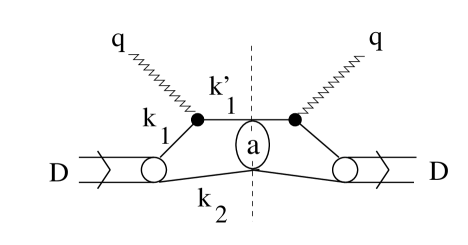
Figure 2: The forward $\gamma^{*}$- d scattering amplitude corresponding to the $p-n$ rescattering in the final state.

The rescattering amplitude, represented by the diagram shown in Fig. 2, has the following form

$${\cal A}_{\mu\nu}=$$ (33)

$$4\gamma^{2}\int\frac{d^{4}k_{1}}{i(2\pi)^{4}}\frac{d^{4}{\tilde{k}}_{1}}{i(2\pi)^{4}}\frac{K_{1\mu}\tilde{K}_{1\nu}\Gamma(k_{1},k_{2})\Gamma(\tilde{k}_{1},\tilde{k}_{2})a(k^{\prime}_{1},k_{2}|\tilde{k}^{\prime}_{1},\tilde{k}_{2})}{(m^{2}-k_{1}^{2})(m^{2}-k_{2}^{2})(m^{2}-k^{\prime\,2}_{1})(m^{2}-\tilde{k}_{1}^{2})(m^{2}-\tilde{k}_{2}^{2})(m^{2}-\tilde{k}^{\prime\,2}_{1})}$$

where $k^{\prime}_{1}=k_{1}+q$, $\tilde{k}^{\prime}_{1}=\tilde{k}_{1}+q$, and $a$ denotes the rescattering amplitude (in the relativistic normalization). The first problem one encounters in the evaluation of Eq. (33), is the integration over the ”-” components of the momenta (light-cone ”energies”). Such an integration requires, in principle, the knowledge of the unknown dependence of both the vertices $\Gamma$ and the rescattering amplitude $a$, upon the ”-” components. In order to overcome such a principle difficulty, we make the approximation consisting of taking into account only the singularities coming from the nucleon propagators in Eq. (33). This can be justified if both the deuteron wave function and the rescattering amplitude are generated by an instantaneous interaction in the light-cone variables, in which case, however, the full relativistic invariance would be lost. Our procedure is equivalent to restoring it by expressing the relativistically invariant arguments via the light-cone variables in the preferable system where the interaction was instantaneous.

It should be pointed out that in the lab system with $q_{+}$ not equal to zero the integration over the ”-” components of the momenta is more complicated than in the system where $q_{+}=0$. Let us choose $k_{2-}$ as an integration variable in the left loop. The three denominators generate three poles in $k_{2-}$:

$$\frac{1}{m_{1\perp}^{2}/2k_{1+}-P_{-}+k_{2-}}\quad\frac{1}{{m^{\prime}_{1\perp}}^{2}/2k^{\prime}_{1+}-P_{-}q_{-}+k_{2-}}\quad\frac{1}{m_{2\perp}^{2}/2k_{2+}-k_{2-}}$$ (34)

where $k^{\prime}_{1}=k_{1}+q$ and all masses are supposed to have a small negative imaginary part. The position of the poles depends on the signs of the $"+"$ components. One has to take into account the following relations, which restrict possible signs of $k_{1,2+}$ and $k^{\prime}_{1+}$:

$$k_{1+}+k_{2+}=P_{+}>0,\ \ k^{\prime}_{1+}=k_{1+}+q_{+}<k_{1+},\ \ k^{\prime}_{1+}+q_{+}>0$$

following from the fact that the $"+"$ component is positive for physical particles and negative for the photon.

One sees immediately that if $k_{2+}<0$ or $k_{2+}>P_{+}$ all poles are on the same side of the real axis in the $k_{2-}$ complex plane, so that the result of the integration will be zero. In fact if $k_{2+}<0$ then both $k_{1+}$ and $k^{\prime}_{1+}$ have to be positive, and all the poles lie above the real axis. If $k_{2+}>P_{+}$, both $k_{1+}$ and $k^{\prime}_{1+}$ are negative and all the poles lie below the real axis.

So, as in the system $q_{+}=0$, we are left with the interval $0<k_{2+}<P_{+}$ and consequently also $0<k_{1+}<P_{+}$. This means that the pole from the spectator nucleon will lie below the real axis, and the one from the active nucleon before the interaction above it. However in the lab system there are two different possibilities for the pole coming from the ejectile propagator: (i) if $k_{2+}<P_{+}+q_{+}$ then $k_{1+}>-q_{+}$ and so $k^{\prime}_{1+}>0$. This is the situation which is always realized in the system $q_{+}=0$, when the ejectile pole lies above the real axis and the total integral is given by the contribution of the residue at the spectator pole at $k_{2}^{2}=m^{2}$, (ii) if $k_{2+}>P_{+}+q_{+}$ and so $k_{1+}<-q_{+}$ then $k^{\prime}_{1+}<0$, the ejectile pole lies below the real axis, and the integral will then be given by the residue at the active nucleon pole $k_{1}^{2}=m^{2}$. Thus the result is different for different values of the scaling variables of the nucleons in the deuteron. Note that in both regions the integrand, apart from the rescattering amplitude and the ejectile propagator, will be expressed via the light-cone function (25) with one of the nucleons on the mass shell. The invariant argument $v$ will however be expressed differently in terms of the integration variables in the described two regions, depending on which of the nucleons lies on the mass shell.

To sum up we get

$${\cal A}_{\mu\nu}=4\gamma^{2}\int d\tau d\tilde{\tau}G(v)G(\tilde{v})K_{\mu}\tilde{K}_{\nu}\frac{a(k^{\prime}_{1},k_{2}|\tilde{k}^{\prime}_{1},\tilde{k}_{2})}{(m^{2}-k^{\prime\,2}_{1})(m^{2}-\tilde{k}^{\prime\,2}_{1})}$$ (35)

where

$$d\tau=d\tau_{2}\equiv\frac{d^{2}k_{2\perp}dx_{2}}{16\pi^{3}x_{2}}\ \ {\rm for}\ \ x_{2}<2+\xi\ \ (x_{1}>-\xi)\ \ {\rm Region\ I}$$ (36)

and

$$d\tau=d\tau_{1}\ \ {\rm for}\ \ x_{1}<-\xi\ \ (x_{2}>2+\xi)\ \ {\rm Region\ II}$$ (37)

In Region I, the virtualities of the active nucleon before and after interaction and the vector $K$, are given by Eqs. (14), (15) and (26) , whereas in Region II one has

$$v=m^{2}-k_{2}^{2}=2\frac{m_{1\perp}^{2}}{x_{1}}-\frac{1}{2}x_{2}M^{2}$$ (38)

$$v^{\prime}=m^{2}-(k_{1}+q)^{2}=Q^{2}\left(1-\frac{x_{1}}{x}\right)+\frac{1}{4}x_{1}\xi M^{2}-\frac{\xi}{x_{1}}m_{1\perp}^{2}$$ (39)

with the four-vector $K$ given by

$$K=k_{1}+yq$$ (40)

where

$$y=\frac{1}{Q^{2}}\left(Q^{2}\frac{x_{1}}{2x}-\frac{1}{8}x_{1}\xi M^{2}+\frac{\xi}{2x_{1}}m_{1\perp}^{2}\right)$$ (41)

The c.m. energy squared for the reaction is given in both regions by Eq. 16. Similar relations hold for variables with tildes in the right integration loop.

Note that in Region II $v^{\prime}=m^{2}-(k_{1}+q)^{2}>0$ and does not vanish. This means that this region gives no contribution to the fast nucleon production.

The four-momentum transfer $t$ in the rescattering is easily calculated to be

$$t=(k_{1}-\tilde{k}_{1})^{2}=(x_{2}-\tilde{x}_{2})\left(\frac{m_{\perp}^{2}}{x_{2}}-\frac{\tilde{m}_{\perp}^{2}}{\tilde{x}_{2}}\right)-(k_{2}-\tilde{k}_{2})_{\perp}^{2},\ \ {\rm Region\ I}$$ (42)

$$t=(x_{2}-\tilde{x}_{2})\left(\frac{1}{2}M^{2}-\frac{m_{\perp}^{2}}{x_{1}}-\frac{\tilde{m}_{\perp}^{2}}{\tilde{x}_{2}}\right)-(k_{2}-\tilde{k}_{2})_{\perp}^{2},\ \ {\rm Region\ II}$$ (43)

In the following we shall introduce a finite formation time for the rescattering by changing the ejectile propagators in the following way

$$\frac{1}{m^{2}-k^{\prime\,2}_{1}}\to\frac{1}{m^{2}-k^{\prime\,2}_{1}}-\frac{1}{{m^{*}}^{2}-k^{\prime\,2}_{1}}$$ (44)

where the subtracted term may be considered as an effective contribution from the excited ejectile states, which makes the rescattering contribution vanish at superhigh energies (equivalent to the colour transparency effect, see [ 3 ]). In our calculations we have chosen $m^{*}=1.8$ GeV.

Contributions to $W_{\mu\nu}$ are obtained from (35) by taking its imaginary part. The latter contains three terms corresponding to cutting the initial or final ejectile propagator (terms 1 and 2) and to cutting the rescattering amplitude. The contribution to $W_{\mu\nu}$ from the 1st term comes only from Region I of the integration over $k_{2}$ (Eq. 36) and is given by

$$W_{\mu\nu}^{1,resc}=4\pi\gamma^{2}\int d\tau_{2}d\tilde{\tau}G(v)G(\tilde{v})\delta(m^{2}-k^{\prime\,2}_{1})K_{\mu}\tilde{K}_{\nu}\frac{a(k^{\prime}_{1},k_{2}|\tilde{k}^{\prime}_{1},\tilde{k}_{2})}{m^{2}-\tilde{k}^{\prime\,2}_{1}-i0}$$

$$=4\gamma^{2}\int dVd\tilde{\tau}G(v)G(\tilde{v})K_{\mu}\tilde{K}_{\nu}\frac{a(k^{\prime}_{1},k_{2}|\tilde{k}^{\prime}_{1},\tilde{k}_{2})}{m^{2}-\tilde{k}^{\prime\,2}_{1}-i0}$$ (45)

where $dV$ is the phase volume (24) of the intermediate real nucleons.

The contribution from the second cut is just the complex conjugate to Eq. (45) with $\mu\leftrightarrow\nu$:

$$W_{\mu\nu}^{2,resc}=\Big{(}W_{\nu\mu}^{1,resc}\Big{)}^{*}$$ (46)

We finally come to the third cut, across the rescattering amplitude. It comes from both Regions I and II and is given by

$$W_{\mu\mu}^{3,resc}=4\gamma^{2}\int d\tau d\tilde{\tau}G(v)G(\tilde{v})K_{\mu}\tilde{K}_{\nu}\frac{{\rm Im}\,a(k^{\prime}_{1},k_{2}|\tilde{k}^{\prime}_{1},\tilde{k}_{2})}{(m^{2}-k^{\prime\,2}_{1}+i0)(m^{2}-\tilde{k}^{\prime\,2}_{1}-i0)}$$ (47)

We shall limit ourselves to the kinematical region of comparatively low energies where the bulk of the contribution to the imaginary part of the rescattering amplitude comes from elastic scattering when

$${\rm Im}\,a(k_{2}|\tilde{k}_{2})=\pi\int d\tau_{2}^{\prime\prime}\delta(m^{2}-k^{\prime\prime\,2}_{1})a(k_{2}|k^{\prime\prime}_{2})a^{*}(k^{\prime\prime}|\tilde{k}_{2})$$ (48)

Putting Eq. (48) into Eq. (47) we get

$$W_{\mu\nu}^{3,resc}=4\gamma^{2}\int dVd\tau d\tilde{\tau}G(v)G(\tilde{v})K_{\mu}\tilde{K}_{\nu}\frac{a(k_{2}|k^{\prime\prime}_{2})a^{*}(k^{\prime\prime}|\tilde{k}_{2})}{(m^{2}-k^{\prime\,2}_{1}+i0)(m^{2}-\tilde{k}^{\prime\,2}_{1}-i0)}$$ (49)

In this formula one has to take $k^{\prime\prime}=p_{1}$, $k^{\prime\prime}_{2}=q+2p-p_{1}$ and express all arguments in terms of light-cone variables of $p_{1}$.

The total rescattering contribution can be represented in a factorized form via the 4-vector

$$X_{\mu}=\int d\tau K_{\mu}G(v)\frac{a(k^{\prime\prime}_{2}|k_{2})}{m^{2}-k^{\prime\,2}_{1}-i0}$$ (50)

where $k^{\prime\prime}_{2}=2p+q-p_{1}$ and $k^{\prime}_{1}=k_{1}+q$ ¿From our formulas we find

$$W_{\mu\nu}^{resc}=4\gamma^{2}\int dV\Big{[}G(v)K_{\mu}X_{\nu}+G(v)K_{\nu}X_{\mu}^{*}+X_{\mu}^{*}X_{\nu}\Big{]}$$ (51)

Adding to this the contribution from the impulse approximation (23) we obtain the total $W_{\mu\nu}$ as an integral of a product of two 4-vectors

$$W_{\mu\nu}^{tot}=4\gamma^{2}\int dVZ^{*}_{\mu}Z_{\nu}$$ (52)

where

$$Z_{i}=G(v)K_{i}+X_{i}$$ (53)

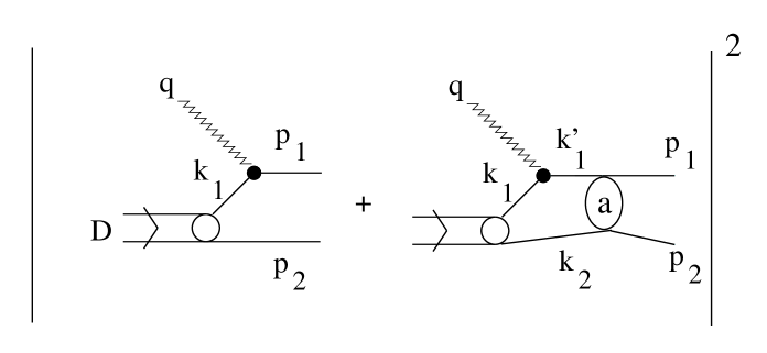
Figure 3: The square of the sum of the impulse approximation and the rescattering amplitudes which govern the inclusive and exclusive cross sections.

Eq. (52) obviously corresponds to the square modulus of the sum of two amplitudes shown in Fig.3

As in the the impulse approximation case, the components of $W_{\mu\nu}$ in the theoretical system are obtained by means of rotation (11). In particular

$$\bar{W}_{++}=4\gamma^{2}\int dV\Big{(}c_{+}Z_{+}+c_{-}Z_{-}+c_{x}Z_{x}\Big{)}^{2}$$ (54)

$$\bar{W}_{yy}=W_{yy}=4\gamma^{2}\int dVZ_{y}^{2}$$ (55)

The longitudinal components of $Z$ do not depend on the azimuthal angle of the observed nucleon $\phi_{1}$. The transverse components have the structure

$$Z_{\perp}=p_{1\perp}\Big{(}G(v)+\frac{|X_{\perp}|}{|p_{1\perp}|}\Big{)}$$ (56)

where the modulus refers only to vector components ($X$ is complex). The integrand in the internal azimuthal integration in $X$ only depends on the azimuthal angle $\phi_{2}$ between $p_{1\perp}$ and $k_{1\perp}$, which enters the transversal part of momentum transfer in the rescattering. If the azimuthal angles of $p_{1\perp}$ and $k_{1\perp}$ are $\phi_{1}$ and $\phi$, we find

$$Z_{x}=\Big{(}|K_{\perp}|G(v)+X_{3}\Big{)}\cos\phi_{1},\ \ Z_{y}=\Big{(}|K_{\perp}|G(v)+X_{3}\Big{)}\sin\phi_{1}$$ (57)

where $X_{3}$ is obtained from $X_{\perp}$ by substituting $k_{1\perp}$ by $|k_{1\perp}|\cos\phi$. Using Eq. (57) one can trivially do the azimuthal integrations in (54) and (55). We obtain in analogy with (30):

$$\sigma_{incl}=\frac{\sigma_{Mott}}{4\pi M}\int d\zeta_{1}J(|{\bf p}_{2}|,x,Q^{2},\theta)$$ (58)

where the integrand is

$$J(|{\bf p}_{2}|,x,Q^{2},\theta)=\frac{\gamma^{2}}{2\pi(2+\xi)}\Big{[}2|c_{+}Z_{+}+c_{-}Z_{-}|^{2}+|Z_{\perp}|^{2}\left(c_{x}^{2}+\tan^{2}(\theta/2)\right)\Big{]}$$ (59)

In PWIA $J\to I$ and becomes directly proportional to the deuteron momentum distribution (c.f. Eq.(31)). The corresponding contribution to the cross-section for the exclusive process can be obtained by removing the integration over $\zeta_{1}$

In Appendix B, some details concerning the calculation of the vector $X$, both in its full relativistic form and within the approximation of Glauber-like rescattering, are given. Here it is instructive to estimate the behaviour of $X$ in the deep cumulative limit. To see this, we have to put in our formulas for $v$ and $t$, $\tilde{x}_{2}=\zeta_{2}\to 0$, keeping $x_{2}$ generally finite as an integration variable. Then one finds, neglecting the transverse motion,

$$t\simeq-\frac{x_{2}}{\zeta_{2}}m^{2}$$ (60)

with $v$ given by

$$v\simeq 2\frac{m^{2}}{x_{2}}$$ (61)

in Region I and by Eq. (38) in Region II. Since $\zeta_{2}\to 0$, $t\to\infty$ unless $x_{2}$ also goes to zero. However then $v\to\infty$ in Region I. Thus, the behaviour of the rescattering contribution, apart from the properties of the ejectile (including the FFT effect), crucially depends upon the relative rate of decrease of the deuteron wave function and the rescattering amplitude as functions of their respective invariant arguments. ¿From general arguments, such a behaviour should be similar in the cumulative limit, since both are generated by the same interaction. In our calculations however we shall represent both behaviours via certain phenomenologically chosen functions. This can be justified up to certain limiting values of $t$ and $v$ below which these approximations are valid. However one is not allowed to come too close to the cumulative limit, where the mutual links between the asymptotic behaviour of $G(v)$ and $a(t)$ becomes crucial.

V Numerical calculations and results

The central quantity we have to calculate is the vector $X_{\mu}$ given by (50). According to Eq. (43), when FFT is taken into account, this vector contains two terms differing in the propagator of the ejectile. Both terms are calculated in a similar manner, the only difference being the mass of the ejectile. Some details of the numerical evaluation of $X_{\mu}$ are given in Appendix B. The basic ingredients entering the definition of $X_{\mu}$ are the relativistic deuteron wave function $G(v)$, the elastic scattering amplitude $a$, and the effective form factor $\gamma$ appearing in the expression of the hadronic tensor. For the relativistic deuteron wave function $G(v)$, we have taken a relativistic generalization of the non-relativistic function $\Psi({\bf k}_{1}^{2})$ which corresponds to the $AV14$ interaction interaction . Its relation to $G(v)$ was established from the non-relativistic limit (see Appendix A), obtaining:

$$G^{2}(v)=2M(2\pi)^{3})|\Psi({\bf k}_{1}^{2})|^{2}$$ (62)

with

$${\bf k}_{1}^{2}=\frac{1}{2}(v-M\epsilon)$$ (63)

As for the rescattering amplitude, it was chosen in the form

$$a(s,t)=(\alpha+i)\sigma^{tot}(s)\sqrt{s(s-4m^{2})}e^{bt}$$ (64)

with the values of the parameters $\sigma^{tot}$, $\alpha$ and $b$ taken from amplitude .

The effective nuclear form-factor $\gamma(Q^{2})$ was chosen to take into account the magnetic interaction of realistic nucleons. A comparison of our impulse approximation results with the results obtained taking spin into accounts in the region of small cumulativity $x\sim 1$ leads to the choice

$$\gamma^{2}(Q^{2})=\gamma_{D}^{2}(Q^{2})\frac{2+\tau(\mu_{p}^{2}+\mu_{n}^{2})}{1+\tau}$$ (65)

where

$$\gamma_{D}(Q^{2})=\left(1+\frac{Q^{2}}{0.71(GeV/c)^{2}}\right)^{-2}$$ (66)

is the dipole ($D$)form-factor, $\tau=Q^{2}/(4m^{2})$, and $\mu_{p,n}$ are the anomalous magnetic moments of the proton and neutron.

To quantify the effects of the non-Glauber nature of the relativistic rescattering we also repeated the calculations taking for the rescattering the Glauber form. This involves two approximations:

1. first, the longitudinal part of the momentum transfer in the rescattering is disregarded, which means that

   $$t=-(k_{2}-\tilde{k}_{2})_{\perp}^{2}$$ (67)

2. second, and most important in our case, the contribution from the real part of the virtual ejectile propagator is neglected, and only the full contribution from its pole is taken into account.

Within the above approximations, evidently, FFT effects vanish unless the rescattering energy becomes greater than the threshold for the production of the excited ejectile with mass $m^{*}$. Our energies lie below this threshold, so that within Glauber rescattering we find no FFT effects.

V.1 The inclusive d(e,e’)np cross section

The cross-section for the inclusive process $d(e,e^{\prime})pn$ is given by Eq. (58), with $J$ given by Eq. (59). Our numerical calculations have been performed in correspondence of the experimental data of expincl with initial electron energy $E=9.761$ GeV and scattering angle $\theta=10^{o}$. We have considered values for the final electron energy which cover the region of $x$ in the interval $1.0<x<1.71$. Some relevant kinematical values characterizing the chosen points are listed in Table 1. It can be seen, as already pointed out in Ref. CKT , that at high values of $x$ (high cumulativity) the value of $p_{lab}$, representing the momentum of the hit nucleon in the lab system of a second nucleon, is very small, well below the threshold energy for pion production. This justifies our approach in terms of nucleon degrees of freedom only, which means that only the elastic rescattering amplitude is used and the excited nucleon states are omitted.

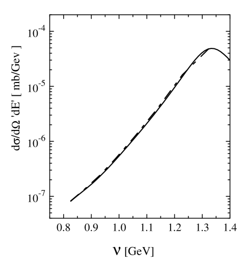
Figure 4: The inclusive cross section calculated in PWIA. Full curve: results of Ref. CKT obtained taking nucleon spin correctly into account; dashed curve: present results based upon spin-less nucleons with the effective form factor given by Eq. 65. In this Figure, as in Figs. 5 and 6, the value of $x$ corresponding to a given value of $\nu$ is listed in Table 1

The IA results calculated within our approach containing the effective form factor given by Eq. (65) is compared in Fig. 4 with the full calculation of Ref. CKT where particle spins are correctly taken into account; it can be seen that the two approaches yield practically the same results. Thus we are confident that the use of spinless particles with effective form factors to take into account rescattering and FFT effects, is a significant one.

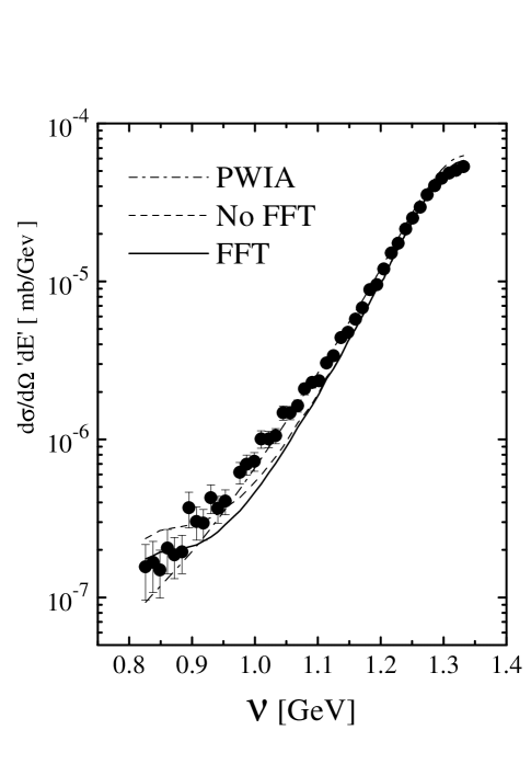
Figure 6: Comparison of the experimental data from Ref. expincl ($E=9.761GeV$) with the results of our calculations corresponding to the PWIA (dot-dash), PWIA plus rescattering (short-dash) and PWIA plus rescattering and FFT (full).

The effects of rescattering and FFT on the inclusive cross section are shown in Figs. 5 and 6 (from now-on, unless differently stated, $FSI$ is used to mean that both rescattering and FFT effects are taken into account). In Fig. 5 we show the ratio of the cross section which includes $FSI$ to the $PWIA$ cross section. It can be seen that that rescattering contributions, which are very small at $x\sim 1$ (corresponding to $\nu\simeq 1.332\,\,GeV$, cf. Table 1), steadily grows with $x$, reaching an order of about 50% already at $x\sim 1.3$. In Fig. 6 and 7 the theoretical results are compared with the experimental data. It can be observed that, up to $x\sim 1.4$ the the cross-section which includes rescattering effects is close to the experimental one at $x\sim 1$ but becomes somewhat lower towards $x=1.4$. Up to $x=1.2$ the FFT effects are negligible but starting from this value tend to substantially diminish the cross-section, whereas above $x=1.4$ the situation abruptly changes: the rescattering strongly enhances the cross-section, an effect which is common to all approaches which take into account FSI (see e.g. Ref. FSIincl ); the effect was found particularly relevant in finite nuclei and various phenomenological effects have been adopted to contrast rescattering effects; from the results presented in Fig. 5, 6 and 7, it can be seen that FFT effects, decreasing the cross section for an off-shell nucleon, lead precisely to the desired effect: when FFT are considered, the cross section is again reduced toward the experimental data. The Glauber approximation seems to work quite well at low cumulativity, $x<1.1$ ($\Delta E>1.2$ GeV). At higher $x$ the Glauber rescattering results are very different from the ones with a full relativistic treatment, both in sign and magnitude. In fact the rescattering in the Glauber approximation gives a relatively small contribution, so that the total cross-section becomes quite close to the impulse approximation. It can be seen that rescattering and FFT effects are necessary in order to improve the agreement at high cumulativity but they tend to destroy the better agreement between experimental data and the PWIA.

V.2 The exclusive d(e,e’p)n cross section

According to (58) the cross section for the exclusive process $d(e,e^{\prime}p)n$ has the following form

$$\sigma_{excl}\equiv\frac{d\sigma}{d\Omega^{\prime}dE^{\prime}d\zeta_{1}}=\frac{\sigma^{Mott}}{4\pi M}J(|{\bf p}_{2}|,x,Q^{2},\theta)$$ (68)

where the definition of $J$ is given by Eq. (59). We will consider the reduced cross section i.e..

$$n_{eff}=|\Psi(|{\bf p}_{2}|)|^{2}\frac{\sigma_{excl}}{\sigma_{excl}^{PWIA}}=|\Psi(|{\bf p}_{2}|)|^{2}\frac{J(|{\bf p}_{2}|,x,Q^{2},\theta)}{I(|{\bf p}_{2}|,x,Q^{2}),\theta}$$ (69)

which, in PWIA turns into the nucleon momentum distribution.

$$n(|{\bf p}_{2}|)=|\Psi(|{\bf p}_{2}|)|^{2}$$ (70)

As already mentioned, the kinematics chosen in the present paper corresponds to small scattering angles $\theta$ l, so that $\theta$-dependence of both $J$ and $I$ coming from terms proportional to $\tan^{2}(\theta/2)$ is negligible.

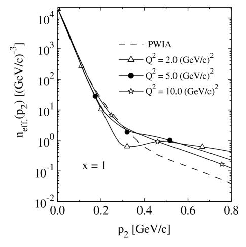
Figure 7: The effective momentum distribution (Eq. 69) vs. the neutron recoil momentum ${|\bf p}_{2}|\equiv p_{2}$ at $x=1$ . The dot-dashed curve represents the PWIA result, whereas the other curves include also rescattering and FFT effects at various values of $Q^{2}$. In this Figure, as in Figures 8-11, $n_{eff}(|{\bf p}_{2}|)\equiv n_{eff}(|{\bf p}_{2}|,x,Q^{2})$.

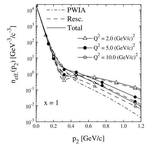
Figure 8: The effective momentum distribution (Eq. 69) at $x=1$ which includes rescattering and FFT effects (full), and rescattering effects only (dashed); the difference between the full and dashed curves is due to FFT effects; the dot-dashed curve represents the PWIA result.

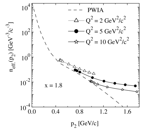
Figure 9: The same as in Fig. 7 at $x=1.8$.

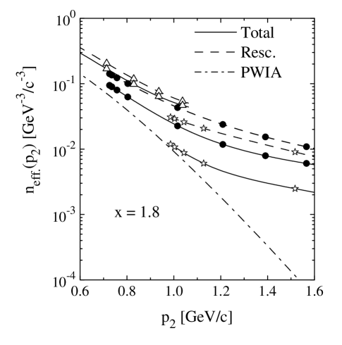
Figure 10: The same as in Fig. 8 at $x=1.8$

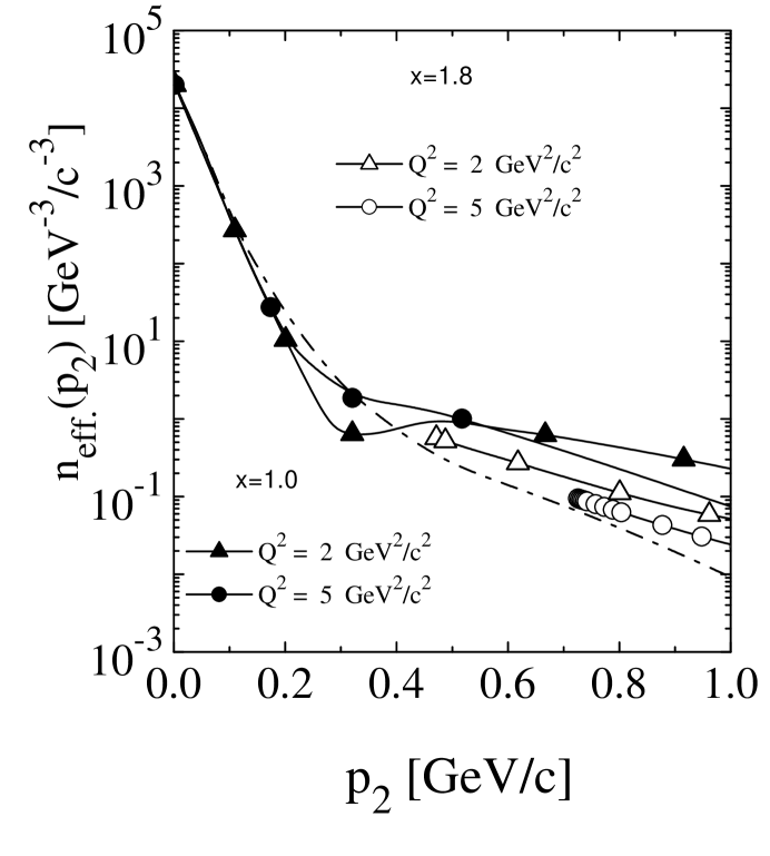
Figure 11: The results of Figs. 7 and 9 are presented here together; the full symbols refer to the effective momentum distribution (Eq. 69) calculated at $x=1$ and the open symbols to $x=1.8$. The dot - dashed curve represents the PWIA.

Figs. 7-11 show the effective momentum distributions calculated taking rescattering and FFT into account. Calculations have been performed fixing the values of $x$ and $Q^{2}$ and varying the missing momentum $|{\bf p}_{mis}|=|{\bf q}-{\bf p}_{1}|=|{\bf p}_{2}|$ which means that, according to the energy conservation of the process, the angle between $|{\bf q}|$ and $|{\bf p}_{2}|$ changes for every value of $|{\bf p}_{2}|$. We have first considered the process at the top of the quasi-elastic peak ($x=1$) and then in the cumulative region ($x>1$). For each value of $x$, calculations have been performed in correspondence of three values of $Q^{2}$, viz. $Q^{2}=2,\,\,5$ and $10(GeV/c)^{2}$.

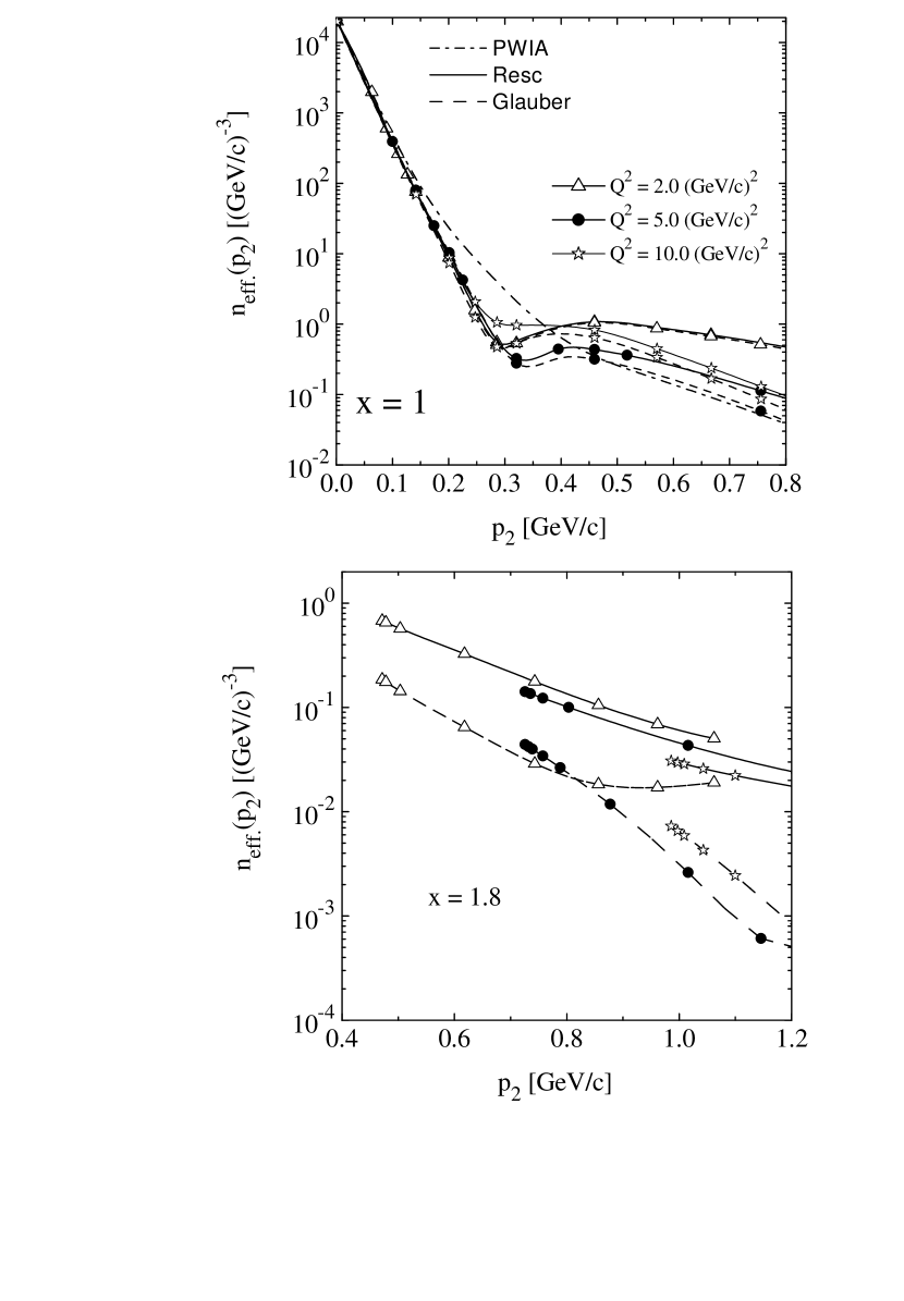
Figure 12: Comparison between the effective momentum distributions (Eq. 69) calculated within our approach (full lines) and within the Glauber approximation (dashed lines); the dot-dashed line represents the PWIA result

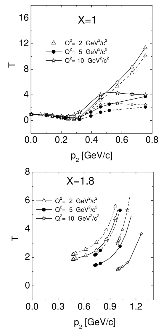
Figure 13: The transparency T, Eq. 71, plotted vs. $|{\bf p}_{2}|\equiv p_{2}$ calculated at $x=1$ and $x=1.8$. The dashed curves represent the PWIA plus rescattering effects, whereas the full curves include also FFT effects.

The results corresponding to $x=1$ are shown in Figs. 7 and 8, whereas the ones corresponding to $x=1.8$ are presented in Figs.  9 and 10. In Fig.7 the nucleon momentum distribution $n(|{\bf p}_{2}|)\equiv n_{eff}^{PWIA}(|{\bf p}_{2}|)$ is compared with $n_{eff}(|{\bf p}_{2}|)\equiv n_{eff}(|{\bf p}_{2}|,x,Q^{2})$ obtained at various values of $Q^{2}$, including both rescattering an FFT effects. The results at $Q^{2}=0.5(GeV/c)^{2}$ show, in agreement with other calculations (see e.g. artmut ), that FSI effects which are very small at $p_{2}\simeq 0$, lead to an appreciable increase of $n_{eff}$ at $p_{2}\geq 0.2GeV/c$ as also recently confirmed by new experimental data ( ulmer ). Fig. 8 illustrates FFT effects, which are given by the difference between the full curves, which include both rescattering and FFT effects, and the dashed curves, which include only rescattering effects. It can be seen that the FFT increases with $Q^{2}$ but, at large values of $Q^{2}$, it seems to decreases, in agreement with the results obtained for the process ${}^{4}He(e,e^{\prime}p)^{3}H$ (FFTHiko ). The results at $x=1.8$ are presented in Figs. 9 and 10. Because of kinematical restrictions imposed by energy conservation, only limited ranges of variation of $p_{2}$ are allowed. Fig. 9 shows that with increasing momentum transfer FSI effects decrease in an appreciable way which is due, as illustrated in Fig. 10, to FFT effects, which makes the distorted cross-section more similar to the PWIA one. Note that in the cumulative region, the effective momentum distribution are lower than the the PWIA results, whereas at $x=1$ one observes the opposite effect. In Fig. 11 $n_{eff}$ at $x=1$ and $x=1.8$ are shown together to illustrate how FSI decrease with $Q^{2}$. Eventually, in Fig. 12, our rescattering results are compared with the Glauber results. It can be seen that with increasing momentum transfer the Glauber approximation provides very poor results, which is particularly true in the cumulativity region. In order to better understand the the difference between the effects of rescattering and and FFT effects, , in Fig. 13 we show the Transparency $T$, defined as

$$T=\frac{n_{eff}^{FSI}(|{\bf p}_{2}|,x,Q^{2})}{n_{eff}(|{\bf p}_{2}|)}$$ (71)

where $n_{eff}^{FSI}$ includes both the rescattering and FFT terms (full lines) or only the rescattering contribution (dashed lines). It can be seen, as already pointed out, that FFT effects lead to opposite results at $x=1$ and in the cumulative regions, respectively, at $x=1$ FFT effects decrease the overall contribution of FSI. In Ref. mark , the process $D(e,e^{\prime}p)n$ has been calculated by treating final state rescattering within the Glauber approach and taking into account colour transparency effects by a quantum diffusion model and by a three-channel approach. Although a direct comparison with the results of Ref. mark is in principle difficult due to the fact that there the variable $\zeta_{2}$ ($\alpha$, in the notation of Ref. mark ) is fixed at $\zeta_{2}=1$, whereas in our kinematical conditions all values of $\zeta_{2}$ allowed by energy conservation are included, a qualitative agreement between the two calculations can be observed.

VI Conclusions

By using a relativistic approach based upon the evaluation of Feynman diagrams, we have calculated the rescattering contribution to the cross-sections of the inclusive, $d(e,e^{\prime})np$, end exclusive, $d(e,e^{\prime}p)n$, processes, paying particular attention to the so-called cumulative region, i.e. the region corresponding to $x>1$. Besides the $p-n$ rescattering in the final state, we have also considered colour transparency effects by introducing the finite formation time of the hit hadron; such an approach, which is simple and physically well grounded, differs from the ones used previously mainly in that the virtuality of the hit nucleon is explicitly taken into account. To make calculation viable, two main approximations have been adopted, namely

1. the nuclear vertex function has been obtained by relativization of the non relativistic deuteron wave function corresponding to the $AV14$ interaction;

2. spin-less nucleons have been considered, but an effective nucleon form factor has been introduced to take into account magnetic moments effects.

Both approximations have been carefully investigated: as far as the first one is concerned, relativistic effects in the nuclear wave function appear to be relevant only at high values of $p_{2}$ and $Q^{2}$ and play a minor role at $p_{2}\leq 0.6(GeV/c)$ and $Q^{2}\leq 5(GeV/c)^{2}$, which is the main region of our investigation; as for the second one, we obtained a good agreement, within the PWIA, between our approach and the results obtained taking spin nucleon spin correctly into account, which makes us confident in our treatment of rescattering and FFT effects.

Concerning the main results we have obtained, they can be summarized as follows:

1. As shown in Figs. 5 and 6, rescattering effects in the inclusive cross section appreciably increase with $x$. At $x\sim 1.4\div 1.5$ they decrease the cross section with respect to the PWIA, in some disagreement with the experimental data. At such values of $x$ the FFT effects reduce the magnitude of rescattering, which changes its relative weight in a very pronounced manner due to interference with the impulse approximation contribution. At still larger values of $x$ rescattering increases the cross-section bringing it into better agreement with the data. This phenomenon may serve to search for FFT or CT effects in the rescattering at comparatively small $Q^{2}$.

2. our results show that at $x=1$ rescattering effects on the exclusive cross section $d(e,e^{\prime}p)n$ become very important at $p_{2}\geq 0.2GeV/c$ and exhibit a strong $Q^{2}$ dependence (cf. Fig. 1), which may serve a significant signal about the nature of rescattering effects. In the cumulative region rescattering effects, at the same value of $Q^{2}$ appear to be less (cf. Fig. 10). As for FFT effects, illustrated in Figs. 8 and 10, they start to be important only at $Q^{2}>5GeV/c$ and high values of $p_{2}$; in particular, at $x>1$ and $Q^{2}=10GeV/c$, they give at $p_{2}\simeq 1.6GeV/c$ a contribution of about an order of magnitude (cf. Fig. 10).

3. we have shown that although the Glauber approximation works quite well at low cumulativity, at high values of $x>>1$ it fails to reproduce our relativistic rescattering both quantitatively and qualitatively.

In conclusions, the results exhibited in this paper demonstrate that the diagrammatic approach we have developed can be successfully applied to the two body case; the application to complex nuclei does not require additional difficulties: it is underway and the results will be presented elsewhere complex .

VII Acknowledgments

We are grateful to B. Kopeliovich for reading the manuscript and useful suggestions. M.A.B and L.P.K. are deeply thankful to the INFN and University of Perugia (Italy) for hospitality and financial support. This work was partly supported by the RFFI Grants 01-02-17137 and 0015-96-737 (Russia).

Appendix A Some details on the numerical calculations

The central quantity we have to calculate is $X_{\mu}$ given by (50). According to (44), when FFT is taken into account, it is a difference of two terms

$$X_{\mu}=X_{\mu}^{(1)}-X_{\mu}^{(2)}$$ (72)

which differ in the propagator of the ejectile. Both terms are calculated in a similar manner, the only difference being the mass of the ejectile. In the following we discuss the first term, not specifying it explicitly.

The components of the vector $K$ (Eq. (40)) have the following values

$$K_{+}=p_{+}\left(2-x_{2}+y\xi\right),\ \ K_{\perp}=-k_{2\perp}$$ (73)

and

$$K_{-}=2p_{-}-\frac{m_{2\perp}^{2}}{2x_{2}p_{+}}+yq_{-},\ \ {\rm Region\ I}$$

$$K_{-}=\frac{m_{1\perp}^{2}}{2x_{1}p_{+}}+yq_{-},\ \ {\rm Region\ II}$$ (74)

where $y$ is given by Eqs. (27) and (41) in Regions I and II respectively.

At a given transverse momentum of the real fast nucleon $p_{1}$, we direct it along the $x$-axis. Then the component $K_{3}$ in $X_{3}$ introduced in the previous section will evidently be

$$K_{3}=|k_{2\perp}|\cos\phi\equiv k\cos\phi$$ (75)

where we denote $k=|k_{2\perp}|$ The rescattering amplitude integrated over the azimuthal angle will give a function

$$b_{\mu}(x_{2},k^{2})=\int_{0}^{2\pi}d\phi a(s,t)\cos^{m}\phi$$ (76)

where $m=0$ for $\mu=\pm$, $m=1$ for $\mu=3$ and $t$ is determined according to Eqs. (42) and (43) in which we have to put $\tilde{x}_{1}=\zeta$ and $\tilde{k}_{1\perp}=p_{1\perp}$.

So after the integration over the azimuthal angles we get

$$X_{\mu}=\frac{1}{32\pi^{3}}\int_{0}^{2}\frac{dx_{2}}{x_{2}}\int_{0}^{\infty}dk^{2}K_{\mu}G(v)b_{\mu}(x_{2},k^{2})\frac{1}{m^{2}-(k_{1}+q)^{2}-i0}$$ (77)

where $\mu=\pm,3$, $K_{3}\to k$, $v$ is given by Eqs. (14) and (38) and the denominator is given by Eqs. (15) and (39).

We put

$$k^{2}=\frac{w}{1-w},\ \ w=\frac{k^{2}}{1+k^{2}},\ \ dk^{2}=\frac{dw}{(1-w)^{2}}$$

to convert the integration region into the interval [0,1]. To separate the singularity in Region I we present the denominator (15) in the form

$$m^{2}-(k_{1}+q)^{2}-i0=\frac{2+\xi}{x_{2}}(k^{2}-\lambda-i0)$$ (78)

where

$$\lambda=-\frac{x_{2}}{2+\xi}\Big{[}Q^{2}\frac{x+x_{2}-2}{x}+m^{2}\frac{2+\xi}{x_{2}}-\frac{1}{4}M^{2}(4-2x_{2}+\xi x_{2})\Big{]}$$ (79)

The singularity is present only if $\lambda>1$. For such $\lambda$ we transform the integral over $k^{2}$ into

$$\frac{x_{2}}{2+\xi}\int_{0}^{1}\frac{dwf(w)}{w-w_{0}-i0}\equiv\frac{x_{2}}{2+\xi}L$$ (80)

where

$$f(w)=\frac{\bar{K}_{\mu}G(v)b_{\mu}(x_{2},k^{2})}{(1-w)(1+\lambda)}$$ (81)

considered as a function of $w$ at fixed $x_{2}$ and

$$w_{0}=\frac{\lambda}{1+\lambda}$$ (82)

If $\lambda>0$ then so $0<w_{0}<1$. We present the integral $L$ as

$$L=\int_{0}^{1}\frac{dw(f(w-f(w_{0}))}{w-w_{0}-i0}+f(w_{0})\left(\ln\frac{1-w_{0}}{w_{0}}+i\pi\right)$$ (83)

The left integral over $w$ has no singularity at $w=w_{0}$ and can be calculated numerically. After that the left integration over $x_{2}$ presents no difficulties in principle.

Appendix B Relation of $G(v)$ to the non-relativistic wave function of the deuteron

We shall find this relation studying the non-relativistic limit. Comparing the diagrams with a direct interaction of the soft photon with the deuteron and via its proton constituent we find

$$2P_{\mu}=\int\frac{d^{4}k_{1}}{(2\pi)^{4}i}2k_{1\mu}G^{2}(v)\frac{1}{m^{2}-k_{2}^{2}}$$ (84)

Taking the zero component and integrating over $k_{20}$ we find

$$2M=\int\frac{d^{3}k_{2}}{(2\pi)^{3}}2k_{10}G^{2}(v)\frac{1}{2k_{20}}$$ (85)

In the nonrelativistic limit $k_{10}=k_{20}=m$ so that we get

$$\int\frac{d^{3}k_{2}}{2M(2\pi)^{3}}G^{2}(v)=1$$ (86)

wherefrom we conclude that

$$G^{2}(v)=2M(2\pi)^{3}\Phi({\bf k}_{2}^{2})$$ (87)

(of course ${\bf k}_{2}^{2}$ can be substituted by ${\bf k}_{1}^{2}$ since ${\bf k}_{1}+{\bf k}_{2}=0$)

Table 1:

$\nu$, GeV	x	$Q^{2},\,(GeV/c)^{2}$	$s,\,GeV^{2}$	$p_{lab},\,GeV/c$
0.826	1.71	2.65	3.96	0.73
0.872	1.61	2.64	4.14	0.88
0.930	1.50	2.62	4.38	1.06
0.987	1.41	2.60	4.61	1.21
1.056	1.30	2.58	4.89	1.40
1.137	1.20	2.56	5.22	1.61
1.228	1.10	2.53	5.58	1.82
1.332	1.00	2.50	6.00	2.07

Some kinematical variables relevant to the experimental data considered in the present paper: $\nu$ is the energy transfer, $x$ the Bjorken scaling variable, $Q^{2}$ the square of the 4- momentum transfer, $s=2m^{2}+2m\sqrt{p_{lab}^{2}+m^{2}}$ the two-nucleon invariant mass in the final state, and $p_{lab}$ the momentum of the struck nucleon in the final state in the lab system of the spectator nucleon. Note that the inelastic channel contributions start to be relevant at $p_{lab}\simeq 1.2\,GeV/c$.

Figure 5: Ratio of the cross section $d\sigma^{FSI}\equiv\frac{d\sigma}{dE^{\prime}d\Omega^{\prime}}$ to the PWIA cross section $d\sigma^{PWIA}\equiv\frac{d\sigma}{dE^{\prime}d\Omega^{\prime}}$. The dashed curve corresponds do $d\sigma^{tot}$ which includes only rescattering effects, whereas the full curve includes both rescattering and FFT effects. The dotted curve corresponds to the Glauber approximation for the rescattering.

References

- (1) L. I. Lapidus, B. Z. Kopeliovich, and A. B. Zamolodchikov, JETP Lett. 33 (1981)612.
- (2) J. Bertch, S. J. Brodsky, A. S. Goldhaber and J. G. Gunion, Phys. Rev. Lett. 47(1981)267.
- (3) A. Mueller, in Proceedings of the 17th Rencontre de Moriond, Ed. by J. Tranh Thanh Van (Editions Frontieres, Gif-sur-Yvette, 1982), p. 13.
- (4) S. J. Brodsky , in Proceedings of the 13th International Symposium on Multiparticle Dynamics, Ed. by E. W. Kittel, W. Metzger, and A. Stergiou (world Scientific, Singapore, 1982), p.964.
- (5) L. L. Frankfurt, G. A. Miller and M. Strikman, Annu. Rev. Part. Sci. 45(1994) 501.
- (6) N. N. Nikolayev, Surveys in High Energy Physics 7(1994) 1.
- (7) V. N. Gribov, Sov. Phys. JETP 29(1969)483; 30 (1970).
-
(8)
G. Garino et al, Phys. Rev. C45 (1992) 780;
N. Makins et al, Phys. Rev. Lett.72 (1994) 1986;
T. O’Neill et al, Phys. Lett. B351 (1995) 87;
D. Abbott et al, Phys. Rev. Lett. 80 (1998) 5072. -
(9)
A. Bianconi, S. Boffi and D. Kharzeev, Phys. Lett.
B305 (1993) 767;
N. N. Nikolaev et al Phys. Lett. B317 (1993) 287;
A. Kohama, K. Yazaki and R. Seki, Nucl. Phys. A551 (1993) 687;
A. S. Rinat and B. K. Jennings, Nucl. Phys. A568 (1994) 873;
L.L. Frankfurt, M. I. Strikman and M. B. Zhalov, Phys. Rev. C50 (1994) 2189;
B. Kopeliovich and J. Nemchik, Phys. Lett. B368 (1996) 187. - (10) B.K.Jennings and B.Z.Kopeliovich, Phys. Rev. Lett., 20 (1993) 3384.
- (11) M. A. Braun, C. Ciofi degli Atti and Treleani, Phys. Rev. C62 (2000) 034606.
-
(12)
C. Ciofi degli Atti, D. Faralli,
A. Yu. Umnikov, and L. P. Kaptari, Phys. Rev. C60 (1999) 034003;
C. Ciofi degli Atti, L. P. Kaptari and D. Treleani, Phys. Rev. C63 (2001) 044601. - (13) R.B. Wiringa, R. A. Smith and T. L. Ainsworth, Phys. Rev. C29 (1984) 1207.
- (14) R. A. Arndt et al., ”Partial-Wave Analysis Facility (SAID)”, http:/said.phys.vt.edu
- (15) S. Rock et al, Phys. Rev. Lett.49 (1982) 1139; R. G. Arnold et al, ibid. 61 (1988) 806.
-
(16)
H. Arhenövel, W. Leidemann, and E. Tomusiak ,
Phys. Rev. C46 (1992) 455;
G. Beck and H Arhenövel, Few-Body Syst. 13 (1992) 165. -
(17)
R. Cenni, C. Ciofi degli Atti, and G. Salme, Phys. Rev. C39 (1989) 1425
O. Benhar, et al, Phys. Rev. C44 (1991) 2328;
A. Kohama, Y. Yazaki, and R. Seki, Nucl. Phys. A662 (2000) 175. - (18) P. E. Ulmer et al, Phys. Rev. Lett. 89 (2002) 062301.
- (19) H. Morita, M. A. Braun, C. Ciofi degli Atti, and D. Treleani, Nucl. Phys. A699 (2002) 328c.
-
(20)
W. Leidemann, E. L. Tomusiak, and H. Arenhoevel, Phys. Rev. C43 (1991) 1022;
F. Ritz, H. Göller, Th. Wilbois, and H. Arhenövel, Phys. Rev. C55 (1997) 2214. - (21) L. L. Frankfurt et al, Phys. Rev. Lett. B369 (1996) 201.
- (22) M. A. Braun, C. Ciofi degli Atti and L. P. Kaptari, in preparation.