$N-d$ scattering including electromagnetic forces

Abstract

The electromagnetic potential consisting in the Coulomb plus the magnetic moment interactions between two nucleons is studied in nucleon-deuteron scattering. For states in which the relative $N-d$ angular momentum $L$ has low values the three–nucleon problem has been solved using the correlated hyperspherical harmonic expansion basis. For states in which the angular momentum $L$ has large values, explicit formulae for the nucleon-deuteron magnetic moment interaction are derived and used to calculate the corresponding $T$-matrices in Born approximation. Then, the transition matrices describing $N-d$ elastic scattering have been derived including an infinite number of partial waves as required by the $1/r^{3}$ behavior of the magnetic moment interaction. Appreciable effects are observed in the vector analyzing powers at low energies. The evolution of these effects by increasing the collision energy is examined.

I Introduction

The study of the magnetic moment interaction (MM) in the two-nucleon ($2N$) system has been subject of many investigations (see Refs. [1, 2] and references there in). Although the intensity of this interaction is very small compared to the nuclear interaction, its long range behavior produces significant effects in nucleon–nucleon ($NN$) scattering. Almost all modern $NN$ potentials have been constructed considering the electromagnetic (EM) interaction used in the Nijmegen partial-wave analysis which includes the MM interaction between the two spin-$\frac{1}{2}$ particles as well as corrections to the $p-p$ Coulomb potential as two-photon exchange, Darwin-Foldy and vacuum polarization terms. When $2N$ scattering observables are computed with one of these potentials the long range behavior of the EM interaction implies an infinite sum in the partial-wave series. For the particular case of the MM interaction, in Refs. [1, 2] it has been shown how to sum analytically these infinite series for $p-p$ and $n-p$ scattering. Important effects of the MM interaction has been observed in both $n-p$ and $p-p$ vector analyzing powers at low energies.

Due to the fact that $2N$ potentials are constructed by fitting the $NN$ available data, the three-nucleon ($3N$) system is the simplest one in which these potentials can be used to make predictions. However, in the description of the $3N$ continuum the MM interaction and corrections to the Coulomb potential has been systematically disregarded. This omission has been justified in the past by the intrinsic difficulties in solving the nuclear problem. At present, the $3N$ continuum is routinely solved by different techniques making possible the treatment of those electromagnetic terms beyond the Coulomb interaction.

In the present paper we study $N-d$ elastic scattering including Coulomb plus MM interactions. Previous description of this process without considering the MM interaction has been performed by the authors using a technique based on the Kohn variational principle (KVP) [3, 4] and expanding the scattering wave function in terms of the correlated hyperspherical harmonics basis [5, 6]. Following these works we perform a partial-wave decomposition of the scattering process. For states with low values of the relative orbital angular momentum $L$ of the projectile and the target, the process is studied by solving the complete $3N$ problem with the Hamiltonian of the system containing nuclear plus Coulomb plus MM interactions. For states with $L$ values sufficiently high, the centrifugal barrier prevents a close approach of the projectile to the target. So, the collision can be considered peripheral and treated as a two-body process. Furthermore, in these states only the EM interaction gives appreciable effects and the corresponding scattering amplitudes can be calculated in Born approximation. The value of $L$ at which the treatment of the problem changes from a three-body description to a two-body description is to some extent arbitrary and could be different at different energies. In practice it can be taken equal to the maximum $L$ value considered when the problem is solved neglecting the MM interaction.

We apply this procedure to calculate the $3N$ vector analyzing powers where the main effects of the MM interaction can be observed. For $p-d$ scattering a sizable increase in $A_{y}$ and $iT_{11}$ has been obtained at low energies which is, however, insufficient to explain the usual underestimation produced by modern $NN$ forces [7, 8]. Other observables as the differential cross section and the tensor analyzing powers suffer minor modifications, of the order of $1$% or less. For $n-d$ scattering a pronounced effect at very small angles is observed. In fact, the scattering amplitude has a term $\sin{\theta}/(1-\cos{\theta})$ which diverges for $\theta\rightarrow 0$ similarly to the $n-p$ case [2]. The experimental observation of this divergence is problematic since it occurs at extreme forward angles (a fraction of degree). This is different from the $p-d$ case in which the Coulomb divergence dominates in that region. Regarding the vector analyzing powers, the MM interaction tends to slightly flatten the $n-d$ $A_{y}$ around the peak and to produce a pronounced dip structure at small scattering angles.

The importance of the EM interaction in the description of $N-d$ scattering decreases as the energy of the process increases. Around $E_{lab}=16$ MeV the improvement given by the MM interaction at the peak of $A_{y}$ and $iT_{11}$ for $p-d$ scattering is already less than $5$%. On the other hand Coulomb effects are important below $E_{lab}=30$ MeV [3]. Here we show that at $E_{lab}=65$ MeV they are considerably reduced in most of the observables with the exception of $T_{21}$ where still some effects can be observed. This analysis will serve to justify the application of standard $n-d$ calculations to the description of $p-d$ scattering at high energies [9].

The paper is organized as follows. In Section II the $N-d$ MM interaction is given. The corresponding $T$-matrices are calculated in Born approximation for both $n-d$ and $p-d$ scattering and final forms for the transition matrices are given. In Section III the transition from a $3N$ description to a $2N$ description is discussed. It is shown that the $3N$ $T$-matrix tends to the $2N$ $T$-matrix as the value of $L$ increases. In Section IV the vector analyzing powers are calculated including the MM interaction and compared to the available data. The differences between the theory and the experiments around the peak of the observables are analyzed. In Section V we present our conclusions. In the Appendix the $n-d$ as well as the $p-d$ MM interactions as two distinctive particles are derived.

II Magnetic Moment Interaction

Following the notation used in the determination of the Argonne $v_{18}$ (AV18) potential [10], all modern $NN$ potentials can be put in the general form

$$v(NN)=v^{EM}(NN)+v^{\pi}(NN)+v^{R}(NN)\ .$$ (1)

The short range part $v^{R}(NN)$ of these interactions includes a certain number of parameters (around 40), which are determined by a fitting procedure to the $NN$ scattering data and the deuteron binding energy (BE), whereas the long range part reduces to the one-pion-exchange potential $v^{\pi}(NN)$ and the electromagnetic potential $v^{EM}(NN)$.

The AV18 potential includes the same $v^{EM}(NN)$ used in the Nijmegen partial-wave analysis except for short-range terms and finite size corrections. The $v^{EM}(pp)$ consists of the one- and two-photon Coulomb terms plus the Darwin-Foldy term, vacuum polarization and MM interactions. The $v^{EM}(np)$ interaction includes a Coulomb term due to the neutron charge distribution in addition to the MM interaction. Finally, $v^{EM}(nn)$ is given by the MM interaction only. All these terms take into account the finite size of the nucleon charge distributions. Explicitly the two–nucleon magnetic moment interaction in the center of mass reference frame reads:

$$v_{MM}(pp) = -{\alpha\over 4M^{2}_{p}}\mu^{2}_{p}\left[{2\over 3}F_{\delta}(r)\mbox{\boldmath$\sigma$}_{i}\cdot\mbox{\boldmath$\sigma$}_{j}+{F_{t}(r)\over r^{3}}S_{ij}\right]$$ (3)

$$-{\alpha\over 2M^{2}_{p}}(4\mu_{p}-1){F_{ls}(r)\over r^{3}}\bf L\cdot\bf S\;\;,$$

$$v_{MM}(np) = -{\alpha\over 4M_{n}M_{p}}\mu_{n}\mu_{p}\left[{2\over 3}F_{\delta}(r)\mbox{\boldmath$\sigma$}_{i}\cdot\mbox{\boldmath$\sigma$}_{j}+{F_{t}(r)\over r^{3}}S_{ij}\right]$$ (5)

$$-{\alpha\over 2M_{n}M_{np}}\mu_{n}{F_{ls}(r)\over r^{3}}(\bf L\cdot\bf S+\bf L\cdot\bf A)\;\;,$$

$$v_{MM}(nn) = -{\alpha\over 4M^{2}_{n}}\mu^{2}_{n}\left[{2\over 3}F_{\delta}(r)\mbox{\boldmath$\sigma$}_{i}\cdot\mbox{\boldmath$\sigma$}_{j}+{F_{t}(r)\over r^{3}}S_{ij}\right]\;\;.$$ (6)

In the above formula $F_{\delta},F_{t}$ and $F_{ls}$ describe the finite size of the nucleon charge distributions. As $r\rightarrow\infty$, $F_{\delta}\rightarrow 0$ whereas $F_{t}\rightarrow 1$ and $F_{ls}\rightarrow 1$. $M_{p}$ ($M_{n}$) is the proton (neutron) mass and $M_{np}$ is the $n-p$ reduced mass. The MM interaction presents the usual $r^{-3}$ behavior and has an operatorial structure with a spin-spin, a tensor and a spin-orbit term. In the $n-p$ case, this last term includes an asymmetric force (proportional to ${\bf A}=$($\sigma$${}_{i}-$$\sigma$${}_{j})/2$) which mixes spin-singlet and spin-triplet states. This term is expected to have a very small effect.

The EM interaction has been studied in the description of bound states in $A\leq 8$ nucleon systems [11]. Recently a detailed analysis of the contribution of the electromagnetic terms to the ³He–³H mass difference has been performed [12]. A first analysis in three–nucleon scattering has been done by Stoks [13] including the MM interaction in Born approximation at high $L$ values. However, the $T$-matrices used at low $L$ values were calculated without considering the MM interaction. In this approximate treatment of the process the main modifications were obtained in the $n-d$ vector analyzing powers at forward angles. No modifications were observed in other observables as the differential cross section and tensor analyzing powers and in the maximum of $A_{y}$ and $iT_{11}$. As a consequence, the conclusion was that the MM interaction does not improve the theoretical underestimation of the last two observables. However, disregarding the MM interaction could not be correct in the description of low partial waves which govern the polarization observables at low energies. In Refs. [14, 15] the MM interaction has been included in the calculation of $N-d$ scattering observables. However in these analyses its contribution was limited to a low number of partial waves. The contribution from waves with high $L$ values was neglected. In the present paper we will include the MM interaction in both regimes in order to perform a complete description of the collision process.

For the case $A=2$, the contribution of the MM interaction to the scattering amplitude has been extensively studied [1, 2]. It has been shown that due to its $r^{-3}$ behavior the scattering amplitude results in a slow convergent series whose leading term can be summed analytically. A similar analysis can be performed for $N-d$ scattering. The starting point is the $N-d$ transition matrix $M$ which can be decomposed as a sum of the Coulomb amplitude $f_{c}$ plus a nuclear term, namely

$$M^{SS^{\prime}}_{\nu\nu^{\prime}}(\theta) = f_{c}(\theta)\delta_{SS^{\prime}}\delta_{\nu\nu^{\prime}}+{\sqrt{4\pi}\over k}\sum_{L,L^{\prime},J}\sqrt{2L+1}(L0S\nu|J\nu)(L^{\prime}M^{\prime}S^{\prime}\nu^{\prime}|J\nu)$$ (8)

$$\,\exp[i(\sigma_{L}+\sigma_{L^{\prime}}-2\sigma_{0})]\;{}^{J}T^{SS^{\prime}}_{LL^{\prime}}\;Y_{L^{\prime}M^{\prime}}(\theta,0)\;\;.$$

This is a $6\times 6$ matrix corresponding to the two possible couplings of the spin $1$ of the deuteron and the spin $1/2$ of the third particle to $S,S^{\prime}=1/2$ or $3/2$ and their projections $\nu$ and $\nu^{\prime}$. The quantum numbers $L,L^{\prime}$ represent the relative orbital angular momentum between the deuteron and the third particle and $J$ is the total angular momentum of the three-nucleon scattering state. ${}^{J}T^{SS^{\prime}}_{LL^{\prime}}$ are the $T$-matrix elements corresponding to a Hamiltonian containing nuclear plus Coulomb plus MM interactions and $\sigma_{L}$ are the Coulomb phase–shifts. The $n-d$ case is recovered putting $f_{c}=\sigma_{L}=0$. When the MM interaction is not considered the sums over $L$, $L^{\prime}$, $J$ converge very fast due to the finite range of the nuclear interactions. Typically in the low energy region ($E_{lab}<50$ MeV) states with $L,L^{\prime}>10$ can be safely neglected. However, when the MM interaction is considered, an infinite number of terms contributes to the construction of the scattering amplitude. In this case the sums on $L,L^{\prime}$ can be divided in two parts. For $L,L^{\prime}\leq L_{max}$ the $T$–matrix elements correspond to, and are obtained from, a complete three-body description of the system. For $L,L^{\prime}>L_{max}$ the centrifugal barrier is sufficiently high to maintain the third particle far from the deuteron and the description of the state can be performed as a two-body system. In general $L_{max}$ can be fixed in such a way that when the collision proceeds in states with $L,L^{\prime}>L_{max}$ the nuclear interaction can be safely neglected and only the Coulomb plus MM potentials contributes to the $N-d$ scattering. It is therefore convenient to introduce the MM interaction between a nucleon and the deuteron as distinct particles. Its specific form can be obtained summing the MM interaction between each nucleon of the deuteron and the third nucleon at large separation distances. Alternatively, the $N-d$ MM interaction can be obtained directly in one-photon exchange approximation between a spin-1 and a spin-1/2 particle from a non-relativistic reduction of the corresponding Feynman diagram. Here below the MM $n-d$ and $p-d$ interactions are explicitly given. The details of the derivation are reserved to the Appendix.

$$v_{MM}(nd) = -{\alpha\over r^{3}}[{\mu_{n}\mu_{d}\over M_{n}M_{d}}S_{nd}^{I}+{\mu_{n}\over 2M_{n}M_{nd}}({\bf L}\cdot{\bf S}_{nd}+{\bf L}\cdot{\bf A}_{nd})]\;\;,$$ (9)

$$v_{MM}(pd) = -{\alpha\over r^{3}}[{\mu_{p}\mu_{d}\over M_{p}M_{d}}S_{pd}^{I}+({\mu_{p}\over 2M_{p}M_{pd}}-{1\over 4M^{2}_{p}})({\bf L}\cdot{\bf S}_{pd}+{\bf L}\cdot{\bf A}_{pd})$$ (11)

$$+({\mu_{d}\over 2M_{d}M_{pd}}-{1\over 4M^{2}_{d}})({\bf L}\cdot{\bf S}_{pd}-{\bf L}\cdot{\bf A}_{pd})-{Q_{d}\over 2}S^{II}_{d}]\;\;,$$

$$S^{I}_{Nd} = 3({\bf S}_{N}\cdot{\hat{r}})({\bf S}_{d}\cdot{\hat{r}})-{\bf S}_{N}\cdot{\bf S}_{d},\;\;\;\;N=n,p$$ (12)

$$S^{II}_{d} = 3({\bf S}_{d}\cdot{\hat{r}})^{2}-2\;\;,$$ (13)

where $M_{d}$ is the deuteron mass, $M_{Nd}$ is the corresponding nucleon-deuteron reduced mass and $\mu_{d}$, $Q_{d}$ are the magnetic and the quadrupole moments of the deuteron, respectively. Moreover, ${\bf S}_{Nd}={\bf S}_{N}+{\bf S}_{d}$ whereas ${\bf A}_{Nd}={\bf S}_{N}-{\bf S}_{d}$. The deuteron-nucleon distance is $r$ and $\hat{r}$ is the unitary vector giving their relative position.

A $n-d$ case

Let us first discuss $n-d$ scattering including the MM interaction. For relative states verifying $L,L^{\prime}>L_{max}$ the description proceeds as a two-body process and the $T$–matrix elements corresponding to a $n-d$ state with total angular momentum $J$, relative angular momentum $L$ and total spin $S$ are given in Born approximation as

$${}^{J}\!T^{LL^{\prime}}_{SS^{\prime}}=-k({2M_{nd}\over\hbar^{2}})<\Omega_{L^{\prime}S^{\prime}J}|v_{MM}(nd)|\Omega_{LSJ}>\;\;.$$ (14)

The relative motion of the $n-d$ system is described by the regular free solution of Schrödinger equation

$$\Omega_{LSJ}=j_{L}(kr)[Y_{L}(\hat{r})\otimes\chi_{S}]_{JJ_{z}}\;\;,$$ (15)

with $k^{2}=(2M_{nd}/\hbar^{2})E_{cm}$, $j_{L}$ a spherical Bessel function and $\chi_{S}$ the total spin function.

The $T$–matrix elements corresponding to the spin-orbit term of the MM interaction proportional to ${\bf L}\cdot{\bf S}+{\bf L}\cdot{\bf A}$ are

$${}^{J}\!T^{LL^{\prime}}_{SS^{\prime}}=-k\;C_{so}<\Omega_{L^{\prime}S^{\prime}J}|{{\bf L}\cdot{\bf S}+{\bf L}\cdot{\bf A}\over r^{3}}|\Omega_{LSJ}>=-k\;C_{so}{\delta_{LL^{\prime}}\over 2L(L+1)}\;\;^{J}\!M^{L}_{SS^{\prime}}\;\;,$$ (16)

with

$$C_{so}=-{\alpha\mu_{n}\over M_{n}}\approx 2.932\times 10^{-3}\;\;{\rm fm}$$ (17)

and

$${}^{J}\!M^{L}_{SS^{\prime}}=(-1)^{L+J+S-S^{\prime}-1/2}\sqrt{6(2S+1)(2S^{\prime}+1)}\left\{\begin{array}[]{rrr}\frac{1}{2}&S^{\prime}&1\\ S&\frac{1}{2}&1\end{array}\right\}\sqrt{L(L+1)(2L+1)}\left\{\begin{array}[]{rrr}S^{\prime}&L&J\\ L&S&1\end{array}\right\}\ .$$ (18)

The $T$-matrix elements of Eq.(16) can be used in Eq.(8) for values of $L,L^{\prime}>L_{max}$. Moreover, for fixed values of $L$ the sum over $J$ can be performed analytically using summation properties of Clebsh-Gordan coefficients. The convergence of the sum on $L$ is slow enough to prevent a safe truncation of the series. Therefore, after summing all terms for $L>L_{max}$, the contribution of the spin-orbit term to the transition matrix of Eq.(8) results:

$$M^{SS^{\prime}}_{\nu\nu^{\prime}}(so)=\frac{C_{so}}{2}K^{SS^{\prime}}_{\nu\nu^{\prime}}\left[\frac{\sin\theta}{1-\cos\theta}-\sum_{L=1}^{L_{max}}\frac{(2L+1)}{L(L+1)}P^{1}_{L}(\cos\theta)\right]\;\;.$$ (19)

$P^{1}_{L}(\cos\theta)$ is a generalized Legendre polynomial and the following property has been used to derive the above equation

$$\sum_{L=1}^{\infty}\frac{(2L+1)}{L(L+1)}P^{1}_{L}(\cos\theta)=\frac{\sin\theta}{1-\cos\theta}\;\;.$$ (20)

Moreover

$$K^{SS^{\prime}}_{\nu\nu^{\prime}}=(-1)^{S-S^{\prime}+\nu+\frac{1}{2}}\sqrt{3(2S+1)(2S^{\prime}+1)}\left\{\begin{array}[]{rrr}\frac{1}{2}&S^{\prime}&1\\ S&\frac{1}{2}&1\end{array}\right\}\left(\begin{array}[]{rrr}S&S^{\prime}&1\\ \nu&-\nu^{\prime}&-M\end{array}\right)\delta_{|M|,1}\;.$$ (21)

As a consequence of the $r^{-3}$ behavior of the MM spin-orbit interaction a term proportional to $\sin\theta/(1-\cos\theta)$ appears in the transition matrix. This term produces a divergence in the differential cross section at extreme forward angles and a pronounced dip structure in the vector analyzing powers.

A similar analysis can be done for the term proportional to the tensor operator in the $n-d$ MM interaction. The corresponding $T$–matrix elements are

$${}^{J}\!T^{LL^{\prime}}_{SS^{\prime}}=-k\;C_{t}<\Omega_{L^{\prime}S^{\prime}J}|{S_{nd}^{I}\over r^{3}}|\Omega_{LSJ}>=-k\;C_{t}\;I_{LL^{\prime}}\;\;^{J}\!M^{LL^{\prime}}_{SS^{\prime}}\;\;,$$ (22)

with

$$C_{t}=-{\alpha\mu_{n}\mu_{d}\over M_{n}+M_{d}}\approx 1.675\times 10^{-3}\;\;{\rm fm}\;\;\ .$$ (23)

The angular-spin and radial matrices are

$${}^{J}M^{LL^{\prime}}_{SS^{\prime}} = (-1)^{L+L^{\prime}+J+S^{\prime}}\left\{\begin{array}[]{rrr}\frac{1}{2}&1&S^{\prime}\\ \frac{1}{2}&1&S\\ 1&1&2\end{array}\right\}$$ (27)

$$\times \sqrt{30(2L+1)(2L^{\prime}+1)(2S+1)(2S^{\prime}+1)}\left\{\begin{array}[]{rrr}L^{\prime}&S^{\prime}&J\\ S&L&2\end{array}\right\}\left(\begin{array}[]{rrr}L&2&L^{\prime}\\ 0&0&0\end{array}\right)$$ (32)

and

$$I_{LL^{\prime}}=\left\{\begin{array}[]{l}\delta_{LL^{\prime}}\over 2L(L+1)\\ \delta_{L+2,L^{\prime}}\over 6(L+1)(L+2)\\ \delta_{L-2,L^{\prime}}\over 6(L^{\prime}+1)(L^{\prime}+2)\end{array}\right.$$ (33)

Again for fixed values of $L$ and $L^{\prime}$ the sum over $J$ in Eq.(8) can be performed analytically and the contribution to the transition matrix is

$$M^{SS^{\prime}}_{\nu\nu^{\prime}}(t) = -\sqrt{4\pi}C_{t}\sqrt{30(2S+1)(2S^{\prime}+1)}\left\{\begin{array}[]{rrr}\frac{1}{2}&1&S^{\prime}\\ \frac{1}{2}&1&S\\ 1&1&2\end{array}\right\}(-1)^{S^{\prime}-\nu}\left(\begin{array}[]{rrr}S&S^{\prime}&2\\ \nu&-\nu^{\prime}&-M\end{array}\right)$$ (39)

$$\times \sum_{L,L^{\prime}>L_{max}}(2L+1)\sqrt{2L^{\prime}+1}I_{LL^{\prime}}\left(\begin{array}[]{rrr}L&L^{\prime}&2\\ 0&0&0\end{array}\right)\left(\begin{array}[]{rrr}L^{\prime}&L&2\\ -M&0&M\end{array}\right)Y_{L^{\prime}M}(\theta,0)\;\;.$$ (44)

Three different sums can be constructed corresponding to $|M|=0,1,2$ that can be summed numerically term by term. The convergence of the series is rather fast and a few tens of terms are sufficient.

In conclusion, the $n-d$ transition matrix including the nuclear plus the MM interaction can be constructed as a sum of three terms

$$M^{SS^{\prime}}_{\nu\nu^{\prime}}(\theta) = {\sqrt{4\pi}\over k}\sum_{L,L^{\prime}}^{L_{max}}\sum_{J}\sqrt{2L+1}(L0S\nu|J\nu)(L^{\prime}M^{\prime}S^{\prime}\nu^{\prime}|J\nu)\;{}^{J}T^{SS^{\prime}}_{LL^{\prime}}\;Y_{L^{\prime}M^{\prime}}(\theta,0)$$ (46)

$$+M^{SS^{\prime}}_{\nu\nu^{\prime}}(so)+M^{SS^{\prime}}_{\nu\nu^{\prime}}(t)\;\;\ .$$

When the MM interaction is neglected only the first term contributes to the transition matrix. When the MM interaction is included, the $T$–matrix elements for $L,L^{\prime}\leq L_{max}$ are different from the previous case. In addition the last two terms in Eq.(46) have to be included. We stress the fact that the value of $L_{max}$ can be taken in such a way that for $L,L^{\prime}>L_{max}$ the nuclear interaction gives a negligible contribution to the scattering process and the interaction between the incident particle and the target is only electromagnetic. Typical values for $L_{max}$ are discussed in Sec.IV.

B $p-d$ case

As for the $n-d$ case, the $T$–matrix elements corresponding to a two-body description of the $p-d$ system with total angular momentum $J$, relative angular momentum $L$ and total spin $S$, are given in Born approximation

$${}^{J}\!T^{LL^{\prime}}_{SS^{\prime}}=-k({2M_{pd}\over\hbar^{2}})<\Omega_{L^{\prime}S^{\prime}J}|v_{MM}(pd)|\Omega_{LSJ}>\;\;.$$ (47)

Here the relative motion of the $p-d$ system is described by

$$\Omega_{LSJ}=F_{L}(\eta,kr)[Y_{L}(\hat{r})\otimes\chi_{S}]_{JJ_{z}}$$ (48)

with $k^{2}=(2M_{pd}/\hbar^{2})E_{cm}$, $F_{L}$ a regular Coulomb function and $\eta$ the usual Coulomb parameter.

Let first consider the spin-orbit terms of the MM interaction in Eq.(11) proportional to $({\bf L}\cdot{\bf S}+{\bf L}\cdot{\bf A})$ and $({\bf L}\cdot{\bf S}-{\bf L}\cdot{\bf A})$. The following matrix elements entering in the calculation of the $T$–matrix are defined

$$<\Omega_{L^{\prime}S^{\prime}J}|{{\bf L}\cdot{\bf S}\pm{\bf L}\cdot{\bf A}\over r^{3}}|\Omega_{LSJ}>=I_{LL^{\prime}}\;\delta_{LL^{\prime}}\;^{J}\!M^{L}_{SS^{\prime}}(\pm)$$ (49)

with [16]

$$I_{LL}=\frac{1}{2L(L+1)}+\frac{1}{2L(L+1)(2L+1)}\left[\eta\pi+1+\eta\pi{\rm coth}\eta\pi-2\eta^{2}\sum_{p=0}^{L}\frac{1}{p^{2}+\eta^{2}}\right]\;\;.$$ (50)

In Eq.(49) the angular-spin matrix $\;{}^{J}\!M^{L}_{SS^{\prime}}(+)$ is equal to the matrix ${}^{J}\!M^{L}_{SS^{\prime}}$ defined in Eq.(18), whereas

$${}^{J}\!M^{L}_{SS^{\prime}}(-)=(-1)^{J+L-1/2}\sqrt{24(2S+1)(2S^{\prime}+1)}\left\{\begin{array}[]{ccc}1&S^{\prime}&\frac{1}{2}\\ S&1&1\end{array}\right\}\sqrt{L(L+1)(2L+1)}\left\{\begin{array}[]{ccc}S^{\prime}&L^{\prime}&J\\ L&S&1\end{array}\right\}.$$ (51)

Following Ref. [1] we isolate the first term of $I_{LL}$ and proceed toward a summation of the related amplitude as we have done for the $n-d$ case. The corresponding contribution to the transition matrix of Eq.(8) for $L>L_{max}$ results

$$M^{SS^{\prime}}_{\nu\nu^{\prime}}(so) = \frac{1}{2}[C^{+}_{so}K^{SS^{\prime}}_{\nu\nu^{\prime}}(+)+C^{-}_{so}K^{SS^{\prime}}_{\nu\nu^{\prime}}(-)]$$ (52)

$$\times \left[\frac{\cos\theta+2{\rm e}^{-i\eta{\rm ln}(\frac{1-\cos\theta}{2})}-1}{\sin\theta}-\sum_{L=1}^{L_{max}}\frac{(2L+1)}{L(L+1)}{\rm e}^{2i(\sigma_{L}-\sigma_{0})}P^{1}_{L}(\cos\theta)\right]\;\;.$$ (53)

To get this final form we have used the following analytical summation of the series [17]

$$\sum_{L=1}^{\infty}\frac{(2L+1)}{L(L+1)}{\rm e}^{2i\sigma_{L}}P^{1}_{L}(\cos\theta)=\frac{{\rm e}^{2i\sigma_{0}}}{\sin\theta}[\cos\theta+2{\rm e}^{-i\eta{\rm ln}(\frac{1-\cos\theta}{2})}-1]\;\;,$$ (54)

which can be obtained from the series of the Coulomb amplitude

$$f_{c}(\theta)=\sum_{L=0}^{\infty}(2L+1)({\rm e}^{2i\sigma_{L}}-1)P_{L}(\cos\theta)=-2i\eta\frac{{\rm e}^{2i\sigma_{0}}}{1-\cos\theta}{\rm e}^{-i\eta{\rm ln}(\frac{1-\cos\theta}{2})}\;\;,$$ (55)

using the recurrence relations of the Legendre polynomials and the following relation of the Coulomb phase-shifts

$${\rm e}^{2i(\sigma_{L}-\sigma_{L-1})}(L-i\eta)=L+i\eta\;\;.$$ (56)

In Eq.(53) $K^{SS^{\prime}}_{\nu\nu^{\prime}}(+)=K^{SS^{\prime}}_{\nu\nu^{\prime}}$ defined in Eq.(21) and

$$K^{SS^{\prime}}_{\nu\nu^{\prime}}(-)=(-1)^{\nu+\frac{1}{2}}\sqrt{12(2S+1)(2S^{\prime}+1)}\left\{\begin{array}[]{rrr}1&S^{\prime}&\frac{1}{2}\\ S&1&1\end{array}\right\}\left(\begin{array}[]{rrr}S&S^{\prime}&1\\ \nu&-\nu^{\prime}&-M\end{array}\right)\delta_{|M|,1}\;\;.$$ (57)

Moreover

$$C_{so}^{+}=-\alpha M_{pd}\left(\frac{\mu_{p}}{M_{p}M_{pd}}-\frac{1}{2M^{2}_{p}}\right)\approx-3.775\times 10^{-3}\;\;{\rm fm}\;\;,$$ (58)

$$C_{so}^{-}=-\alpha M_{pd}\left(\frac{\mu_{d}}{M_{d}M_{pd}}-\frac{1}{2M^{2}_{d}}\right)\approx-5.936\times 10^{-4}\;\;{\rm fm}\;\;.$$ (59)

The term proportional to $C_{so}^{-}$ is much smaller due to the small magnetic moment of the deuteron. The same happens to the term proportional to $Q_{d}$ in Eq.(11) due to the small quadrupole moment of the deuteron and will not be discussed here. The analysis of the term proportional to the tensor operator in the MM interaction proceeds similarly to that one performed in the $n-d$ case, taking care that now the radial integral $I_{LL}$ is given by Eq.(50) and $I_{L,L+2}=\frac{1}{6}|L+1+i\eta|^{-1}|L+2+i\eta|^{-1}$ [16]. In conclusion the transition matrix can be constructed as a sum of different contributions

$$M^{SS^{\prime}}_{\nu\nu^{\prime}}(\theta) = f_{c}(\theta)\delta_{SS^{\prime}}\delta_{\nu\nu^{\prime}}+{\sqrt{4\pi}\over k}\sum_{LL^{\prime}}^{L_{max}}\sum_{J}\sqrt{2L+1}(L0S\nu|J\nu)(L^{\prime}M^{\prime}S^{\prime}\nu^{\prime}|J\nu)$$ (60)

$$\times \,\exp[i(\sigma_{L}+\sigma_{L^{\prime}}-2\sigma_{0})]\;{}^{J}T^{SS^{\prime}}_{LL^{\prime}}\;Y_{L^{\prime}M^{\prime}}(\theta,0)+M^{SS^{\prime}}_{\nu\nu^{\prime}}(so)+B^{SS^{\prime}}_{\nu\nu^{\prime}}\;\;,$$ (61)

where $M^{SS^{\prime}}_{\nu\nu^{\prime}}(so)$ is defined in Eq.(53) and $B^{SS^{\prime}}_{\nu\nu^{\prime}}$ includes the contribution of the remaining terms in Eq.(50) and those coming from the tensor operator. The $B^{SS^{\prime}}_{\nu\nu^{\prime}}$ matrix elements can be evaluated summing the corresponding series numerically for $L,L^{\prime}>L_{max}$ until convergence is reached.

III The $3N$ and $N-d$ $T$-matrices in Born approximation

The calculations of the observables in $N-d$ scattering can be obtained from the transition matrices of Eqs.(46) and (61). Accordingly, after a partial wave decomposition, it is necessary to calculate the three-nucleon $T$–matrices for states with total angular momentum $J$ in which the deuteron and the incident nucleon are in relative motion in the regime $L\leq L_{max}$. As discussed before, states having $L>L_{max}$ are described as a two-body process. Therefore it is appropriate to make a link between the two regimes and show in which manner the three-nucleon $T$–matrix smoothly tends to a two-body $T$–matrix as $L$ increases.

The KVP in its complex form establishes that the $T$-matrix elements are functionals of the three-nucleon scattering state

$$[{}^{J}\!{T}^{SS^{\prime}}_{LL^{\prime}}]={}^{J}\!{T}^{SS^{\prime}}_{LL^{\prime}}-\frac{M}{2\sqrt{3}\hbar^{2}}\langle\Psi^{-}_{LSJ}|H-E|\Psi^{+}_{L^{\prime}S^{\prime}J}\rangle\ .$$ (62)

The stationarity of this functional with respect to the trial parameters in the three–nucleon scattering state $\Psi^{+}_{LSJ}$ is required to obtain the $T$–matrix first order solution. The second order estimate is obtained after replacing the first order solution in Eq.(62). In this formalism [18] the continuum state is usually written as a sum of three Faddeev-like amplitudes, each of which consists of two terms:

$$\Psi^{+}_{LSJ}=\sum_{i=1,3}\left[\Psi_{C}({\bf x}_{i},{\bf y}_{i})+\Omega^{+}_{LSJ}({\bf x}_{i},{\bf y}_{i})\right]\;\;\;,$$ (63)

here ${\bf x}_{i},{\bf y}_{i}$ are the Jacobi coordinates corresponding to the $i$–th permutation of the particles indices $1,2,3$. The first term, $\Psi_{C}$, describes the system when the three–nucleons are close to each other. For large interparticle separations and energies below the deuteron breakup threshold it goes to zero, whereas for higher energies it must reproduce a three outgoing particle state. The second term, $\Omega^{+}_{LSJ}$, describes the asymptotic configuration of a deuteron far from the third nucleon and explicitly it is:

$$\Omega^{+}_{LSJ}({\bf x}_{i},{\bf y}_{i})=\Omega^{0}_{LSJ}({\bf x}_{i},{\bf y}_{i})+\sum_{L^{\prime}S^{\prime}}{}^{J}\!T^{SS^{\prime}}_{LL^{\prime}}\Omega^{1}_{L^{\prime}S^{\prime}J}({\bf x}_{i},{\bf y}_{i})\ ,$$ (64)

where

$$\Omega^{0}_{LSJ}({\bf x}_{i},{\bf y}_{i}) = \Omega^{R}_{LSJ}({\bf x}_{i},{\bf y}_{i})$$ (65)

$$\Omega^{1}_{LSJ}({\bf x}_{i},{\bf y}_{i}) = \Omega^{R}_{LSJ}({\bf x}_{i},{\bf y}_{i})-i\Omega^{I}_{LSJ}({\bf x}_{i},{\bf y}_{i})\ .$$ (66)

Besides a factor $\sqrt{k}$, $\Omega^{R}_{LSJ}$ is the function $\Omega_{LSJ}$ given in Eqs.(15) and (48) for the $n-d$ and $p-d$ system respectively, in which $\chi_{S}$ represents the deuteron wave function of spin $1$ coupled with the spin $\frac{1}{2}$ of the third nucleon to total spin $S$. In $\Omega^{I}_{LSJ}$ the regular relative function $j_{L}$ or $F_{L}$ is replaced by the corresponding irregular solution $\eta_{L}$ or $G_{L}$ regularized at the origin[5]. The normalization of the asymptotic states verifies

$$\frac{M}{2\sqrt{3}\hbar^{2}}\sum_{i,j}[\langle\Omega^{R}_{LSJ}({\bf x}_{i},{\bf y}_{i})|H-E|\Omega^{I}_{L^{\prime}S^{\prime}J}({\bf x}_{j},{\bf y}_{j})\rangle-\langle\Omega^{I}_{LSJ}({\bf x}_{i},{\bf y}_{i})|H-E|\Omega^{R}_{L^{\prime}S^{\prime}J}({\bf x}_{j},{\bf y}_{j})\rangle]=1\;\;,$$ (67)

$M$ being the nucleon mass. To be noticed that in the three-nucleon process the energy in the center of mass reference frame is

$$E={4Mk^{2}\over 3\hbar^{2}}+E_{d}={2M_{Nd}k^{2}\over\hbar^{2}}+E_{d}$$ (68)

with $E_{d}$ the deuteron ground state energy. Moreover, the factor $1/(2\sqrt{3})$ in Eq.(67) is related to the definitions of the Jacobi coordinates in terms of the particle coordinates:

$${\bf x}_{i} = {\bf r_{j}}-{\bf r_{k}}$$ (69)

$${\bf y}_{i} = \frac{2}{\sqrt{3}}({\bf r_{k}}-\frac{{\bf r_{i}}+{\bf r_{j}}}{2})\ .$$ (70)

The Born approximation of the $T$-matrix is obtained from Eq.(62) replacing the wave function $\Psi$ by the regular function $\Omega^{0}$ and putting the first order $T$-matrix equal to zero:

$$[{}^{J}\!{T}^{SS^{\prime}}_{LL^{\prime}}]_{B}=-\frac{M}{2\sqrt{3}\hbar^{2}}\sum_{i,j}\langle\Omega^{0}_{LSJ}({\bf x}_{i},{\bf y}_{i})|H-E|\Omega^{0}_{L^{\prime}S^{\prime}J}({\bf x}_{j},{\bf y}_{j})\rangle\ .$$ (71)

For a given energy a certain value $L_{B}$ exists such that for $L,L^{\prime}\geq L_{B}$ the differences between the $T$–matrix elements obtained from a complete solution of the three-nucleon problem or from its Born approximation are extremely small. Increasing further the values of $L$ and $L^{\prime}$ we arrive to the regime $L,L^{\prime}>L_{max}$ in which the contribution of the $NN$ nuclear potential can be neglected. Let us consider ${\bf x}_{3},{\bf y}_{3}$ the Jacobi coordinates corresponding to the asymptotic configuration in which nucleons ($1,2$) form the deuteron and nucleon $3$ is the incident particle. The relative coordinate between the third nucleon and the center of mass of the deuteron is ${\bf r}_{Nd}=(\sqrt{3}/2){\bf y}_{3}$. Starting from the above Born approximation for the $T$-matrix, the following relations are verified for $L,L^{\prime}>L_{max}$:

$$[{}^{J}{T}^{SS^{\prime}}_{LL^{\prime}}]_{B} = -\frac{M}{2\sqrt{3}\hbar^{2}}\sum_{i,j}\langle\Omega^{0}_{LSJ}({\bf x}_{i},{\bf y}_{i})|H-E|\Omega^{0}_{L^{\prime}S^{\prime}J}({\bf x}_{j},{\bf y}_{j})\rangle$$ (72)

$$= -3\frac{M}{2\sqrt{3}\hbar^{2}}\sum_{i}\langle\Omega^{0}_{LSJ}({\bf x}_{i},{\bf y}_{i})|V(1,3)+V(2,3)|\Omega^{0}_{L^{\prime}S^{\prime}J}({\bf x}_{3},{\bf y}_{3})\rangle$$ (73)

$$\approx -3\frac{M}{2\sqrt{3}\hbar^{2}}\langle\Omega^{0}_{LSJ}({\bf x}_{3},{\bf y}_{3})|V(1,3)+V(2,3)|\Omega^{0}_{L^{\prime}S^{\prime}J}({\bf x}_{3},{\bf y}_{3})\rangle$$ (74)

$$\approx -3\frac{M}{2\sqrt{3}\hbar^{2}}\langle\Omega^{0}_{LSJ}({\bf x}_{3},{\bf y}_{3})|v_{MM}(Nd)|\Omega^{0}_{L^{\prime}S^{\prime}J}({\bf x}_{3},{\bf y}_{3})\rangle$$ (75)

$$= -2k\frac{M_{Nd}}{\hbar^{2}}\langle\Omega_{LSJ}|v_{MM}(Nd)|\Omega_{L^{\prime}S^{\prime}J})\rangle\ .$$ (76)

The equivalence between the second and third row is in general verified for $L,L^{\prime}>L_{B}$. On the other hand, the equivalence between the third and fourth row is verified for $L,L^{\prime}>L_{max}$. In fact, $L_{max}$ can be fixed as the $L$ value at which these two rows start to be approximately equal. Finally, in the last step the asymptotic three-nucleon function $\Omega^{0}$ has been replaced by the two-body function $\Omega$ of Eq.(15) once the integration over ${\bf x}_{3}$ and the change of variables ${\bf y}_{3}\rightarrow{\bf r}_{Nd}$ has been performed. In conclusion, the above approximate equalities show the relation between the three–nucleon $T$–matrix of Eq.(71) and the two-body $T$–matrices of Eqs.(14) and (47) for high $L$ values.

IV $N-d$ observables including Coulomb plus MM interactions

Elastic observables for $N-d$ scattering can be calculated using the transition matrices of Eqs.(46) and (61) using trace operations [19]. The calculations presented here have been performed using the KVP after an expansion of the three-nucleon scattering wave function in terms of the pair correlated hyperspherical harmonic (PHH) basis [5, 6]. As $NN$ interaction we have used the nuclear part of the AV18 potential plus the Coulomb and MM interactions defined in Eqs.(3)-(6). The asymmetric force ${\bf L}\cdot{\bf A}$ in the $v_{MM}(np)$ interaction has been included as well as the $p-p$ Darwin-Foldy and the $n-p$ short-range Coulomb terms.

At energies below the deuteron breakup threshold the contribution of the MM interaction is expected to be appreciable. Recently the $n-d$ analyzing power $A_{y}$ has been measured at $E_{lab}=1.2$ and $1.9$ MeV [20]. At these very low energies the nuclear part of the transition matrix (first term of Eq.(46)) converges already for $L_{max}=3$. The corresponding theoretical curves obtained using the AV18 potential, and neglecting the MM interaction, are showed in Fig.1 (solid line). As it can be seen, the observable is not reproduced by a large amount which is a common feature of all modern $NN$ forces. When the MM interaction is taken into account up to $L_{max}=3$, the analyzing powers are given by the dashed curves. There is a very small influence of the MM interaction in the peak of $A_{y}$ with the tendency of slightly flattening the observable. However, this is an incomplete calculation since the inclusion of the MM interaction requires an infinite number of partial waves in the calculation of the transition matrix. When all three terms of Eq.(46) are considered the observables are given by the dashed-dotted curves. It is interesting to notice the forward-angle dip structure which already appears in $n-p$ scattering [2]. Only after summing the series up to $\infty$ this particular behavior can be reproduced. We can conclude that the MM interaction produces a pronounced modification of $A_{y}$ at forward angles but has a very small effect around the peak.

In order to show the importance of the MM moment interaction in the calculations of $A_{y}$ as the energy increases, in Fig.2 the results at $E_{lab}=6.5$ MeV are given. At this particular energy $A_{y}$ has been measured in an extended angular range including forward angles [21]. The solid line corresponds to a standard AV18 calculation neglecting the MM interaction and including partial waves up to $L_{max}=8$. The dashed-dotted line corresponds to a calculation using the AV18+MM potential and considering the complete series. We can observe that the effect of the MM interaction on the peak is practically negligible. Conversely, it is of great importance at forward angles in order to describe the zero crossing.

Besides the neutron analyzing power and the deuteron analyzing power which present similar characteristics, other elastic $n-d$ observables as the tensor analyzing powers suffer only minor modifications when the MM interaction is included. The differences are of the order of $1$% or less and they are not presented here. However when comparisons with precise experimental data are performed these differences could be relevant and the MM interaction should be taking into account.

For $p-d$ scattering high precision data exist at low energies [22, 23, 24, 25] for differential cross section and vector and tensor analyzing powers. Detailed comparisons to these data has been performed in Refs. [7, 22, 23, 26] using AV18 with and without the inclusion of three–nucleon forces. In those studies the Coulomb interaction was included whereas the MM interaction was not. In order to evaluate the effects of the MM interaction on the vector analyzing powers in presence of the Coulomb field, in Fig.3 the results of the calculations at $E_{p}=1$ and $3$ MeV are shown. Three different calculations have been performed at both energies. The solid line corresponds to the AV18 prediction neglecting the MM interaction. Accordingly, the transition matrix has been calculated with the first two terms of Eq.(61). The partial-wave series of the second term has been summed up to $L_{max}=4$ ($E_{p}=1$ MeV) and $L_{max}=6$ ($E_{p}=3$ MeV). The dashed line corresponds to the same calculation as before but the $T$-matrix elements has been calculated using the AV18+MM potential. The dashed-dotted line corresponds to the complete calculation including also the last two terms of Eq.(61). We see that the major effect of the MM interaction is obtained around the peak and is appreciable at both energies. There is also an improvement in the description of the observable at forward angles, in particular for $iT_{11}$ at $E_{p}=3$ MeV. The observed modifications are due to the interference between the Coulomb and the nuclear plus the MM interaction and not to higher order terms, as in the $n-d$ case, since, except for $A_{y}$ at $E_{p}=1$ MeV, the dashed and dashed-dotted line practically overlap. In fact, high order terms are dominated by the Coulomb interaction and the MM interaction gives a very small contribution.

As the energy increases, the effect of the MM interaction on $A_{y}$ and $iT_{11}$ diminishes as it is shown in Fig.4 at $E_{p}=5$ and $10$ MeV. Here the AV18 prediction (solid line) has to be compared to the AV18+MM prediction (dashed line) calculated using the first two terms of Eq.(61) with $L_{max}=8$. When the last two terms of Eq.(61) are also included, the results are extremely close to the previous ones. As for the $n-d$, the tensor analyzing powers present very small modifications when the MM interaction is taking into account and are not presented here.

The MM interaction has different effects in $n-d$ or $p-d$ vector analyzing powers. One reason is the different sign between the neutron and proton magnetic moment. Another reason is the interference with the Coulomb field. However the MM interaction does not help for a better description of the neutron $A_{y}$. On the contrary there is an appreciable improvement in the proton $A_{y}$ as well as in $iT_{11}$, in particular at very low energies. Hence we can examine the differences between the experimental data and the theory at the peak in order to see if the inclusion of the MM interaction helps to clarify a different behavior observed for $n-d$ and $p-d$. In Fig.5 the relative difference $[A_{y}(exp)-A_{y}(th)]/A_{y}(exp)$ at the peak for $n-d$ and for $p-d$ scattering is shown. In this last case both, the AV18 and AV18+MM results have been reported. For $n-d$ both results are extremely close at the peak, so the difference does not depend on which calculation (AV18 or AV18+MM) is considered. Without the inclusion of the MM interaction the underestimation of the proton $A_{y}$ is much more pronounced than the neutron $A_{y}$. When the MM interaction is considered the difference between theory and experiment for both, $p-d$ and $n-d$ scattering are of similar size, around $25$%, for all the energy values below $16$ MeV. Above $16$ MeV the differences at the peak between theory and experiment diminish. As shown in Fig.5, at $18$ MeV the difference is around $20$%. In Fig.6 the deuteron analyzing power $iT_{11}$ is examined. The relative difference $[iT_{11}(exp)-iT_{11}(th)]/iT_{11}(exp)$ is shown at the peak for $p-d$ scattering (there is no data for the $n-d$ case) using AV18 and AV18+MM. Besides the first point at $E_{lab}=0.650$ MeV which corresponds to a very small value of $iT_{11}$ [22], the underestimation of the observable oscillates around $24$%, very close to the $A_{y}$ case.

Finally we wish to discuss the importance of the Coulomb effects as the energy increases. In fact, up to $E_{lab}=30$ MeV we can observe appreciable differences in the description of $n-d$ and $p-d$ elastic scattering that however tend to diminish [3]. Experimental data are not always conclusive since experiments with neutrons have larger uncertainties than those performed with protons. On the other hand, $n-d$ calculations have been often used to describe $p-d$ scattering, in particular at high energies [9]. In order to clarify this approximation, in Figs.7–8 $n-d$ and $p-d$ calculations at $E_{lab}=65$ MeV are compared. To make contact with the results given in Ref. [9] in which $n-d$ scattering has been analyzed at this particular energy, we have consider also the Urbana IX (UR) three–nucleon interaction [31]. In Fig.7 the differential cross section and $A_{y}$ are shown. Three curves are displayed corresponding to $p-d$ AV18 (solid line), $n-d$ AV18 (dashed line) and $p-d$ AV18+UR (dotted line) and compared to the experimental data. In Fig.8 the same calculations are shown for $iT_{11}$ and the three tensor analyzing powers $T_{20},T_{21}$ and $T_{22}$. As expected, Coulomb effects are small at this energy. We can observe appreciable Coulomb effects only in $T_{21}$ whereas three-nucleon interaction effects are found in the minimum of the differential cross section and in $T_{21}$ and $T_{22}$ as well. These results justify to some extent the description of $p-d$ data using $n-d$ calculations at intermediate energies, however with some caution in the description of particular observables.

V conclusions

The MM interaction has been included in the description of $N-d$ scattering at low energies. Though its strength is small compared to the nuclear interaction, it has a very long tail which behaves as $1/r^{3}$. As a consequence, the construction of the scattering amplitude necessitates an infinite number of partial waves. Analytical summations of the corresponding $p-d$ and $n-d$ series have been given following previous works for $NN$ scattering. Accordingly, the $6\times 6$ transition matrix $M$ has been written as a sum of the standard Coulomb amplitude plus the MM amplitude and a finite series of $T$–matrices. These matrices have been calculated from a complete three–body description of the process with a Hamiltonian including the nuclear plus Coulomb plus MM interaction. For high $L$ values, the MM amplitude has been calculated as a two-body process. To this aim the MM interaction between a nucleon and the deuteron as distinct particles has been derived.

Different $3N$ elastic observables have been calculated and compared to previous calculations in which the MM interaction was neglected. The main effect has been observed in the vector analyzing powers. However the modifications produced by the MM interaction do not improve the description of the neutron $A_{y}$ around the peak. Conversely, there is an appreciable improvement in the proton $A_{y}$ and in $iT_{11}$, in particular at low energies. Due to the different effect that the MM interaction produces in $n-d$ and $p-d$ scattering, the relative difference between the calculated and the measured $A_{y}$ at the peak results largely charge independent and approximately constant below $16$ MeV. The underestimation is about $25$%. Above this energy the difference starts to diminish. At $E_{lab}=18$ MeV it has been reduced to $20$% and above $30$ MeV there is a much better description of $A_{y}$ and $iT_{11}$. This is shown by the calculations performed at $E_{lab}=65$ MeV. Furthermore, we have shown that at this energy Coulomb effects are not important. Only $T_{21}$ still shows some sensitivity.

The main aim of this work is to describe the three–nucleon continuum using the same $v^{EM}(NN)$ used in the description of the $2N$ scattering states. In the past the MM interaction has been systematically neglected in the calculation of $3N$ scattering observables with few exceptions. Here we show how to include it and which terms are important. From the present analysis it can be concluded that the approximate treatment of Ref. [13] is justified for $n-d$ scattering but not for the $p-d$ case. In fact, in the calculation of the $n-d$ $A_{y}$ the symmetric spin–orbit term in $v_{MM}(np)$ tends to depress the observable at the peak whereas the asymmetric term almost cancel this effect. Therefore the transition matrix of Eq.(46) can be constructed with the MM amplitudes $M^{SS^{\prime}}_{\nu\nu^{\prime}}(so)$ and $M^{SS^{\prime}}_{\nu\nu^{\prime}}(t)$ but neglecting the MM interaction in the calculation of the $T$-matrix elements ${}^{J}\!T^{SS^{\prime}}_{LL^{\prime}}$ for $L,L^{\prime}<L_{max}$. In addition, the amplitude $M^{SS^{\prime}}_{\nu\nu^{\prime}}(t)$ gives an extremely low contribution and can be neglected too. In the $p-d$ case the interference between the Coulomb, MM and nuclear interactions does not allow for the omission of the MM interaction in the calculation of the $T$–matrix elements. Otherwise the improvement at low energies on the peak of $A_{y}$ and $iT_{11}$ is lost. However, in the construction of the transition matrix the last two terms in Eq.(61) give very small contributions and, except at extremely low energies, can be omitted.

Other small terms in the $v^{EM}(pp)$ interaction as the two-photon Coulomb and vacuum polarization interactions have been neglected in the present analysis. These terms have improved the description of $p-p$ scattering at low energies and, therefore, their inclusion in the description of $p-d$ scattering is of interest. The analysis of these terms as well as the study of the MM interaction in $p-^{3}$He scattering is at present underway.

A

In this appendix we briefly outline the derivation of the $N-d$ MM interactions of Eqs. (9) and (13).

We consider two particles, the first one with spin 1/2, mass, charge and magnetic moment $M_{1}$, $Z_{1}$ and $\mu_{1}$, respectively, the second one with spin 1, mass, charge, magnetic moment and quadrupole moment $M_{2}$, $Z_{2}$, $\mu_{2}$ and $Q_{2}$, respectively. The magnetic and the quadrupole moments are given in n.m. and fm², respectively. The non-relativistic reduction of the covariant current for the point-like spin-1/2 particle gives for the charge $\rho$ and current ${\bf j}$ operators in $r$-space [32]:

$$\rho_{1}({\bf q}) = Z_{1}{\rm e}^{i{\bf q}\cdot{\bf r}_{1}}-i\,\frac{2\mu_{1}-Z_{1}}{2M_{1}^{2}}{\bf q}\cdot({\bf S}_{1}\times{\bf p}_{1}){\rm e}^{i{\bf q}\cdot{\bf r}_{1}}\ ,$$ (A1)

$${\bf j}_{1}({\bf q}) = \frac{Z_{1}}{2M_{1}}\{{\bf p}_{1},{\rm e}^{i{\bf q}\cdot{\bf r}_{1}}\}-i\,\frac{\mu_{1}}{M_{1}}({\bf q}\times{\bf S}_{1}){\rm e}^{i{\bf q}\cdot{\bf r}_{1}}\ ,$$ (A2)

where ${\bf q}$ is the three-momentum transferred to the particle, ${\bf p}_{1}$ and ${\bf S}_{1}$ are the momentum and spin operators, respectively, and $\{\cdots,\cdots\}$ denotes the anticommutator. We have here neglected the Darwin-Foldy relativistic correction.

The covariant current operator for a spin-1 particle is written as [33]

$$j^{\mu} = -\frac{1}{\sqrt{4E\,E^{\prime}}}\{[G_{1}(Q^{2})(\epsilon^{\prime*}\cdot\epsilon)-\frac{G_{3}(Q^{2})}{2M_{2}^{2}}(\epsilon^{\prime*}\cdot q)(\epsilon\cdot q)]P^{\mu}$$ (A4)

$$+G_{2}(Q^{2})[\epsilon^{\mu}(\epsilon^{\prime*}\cdot q)-\epsilon^{\prime*\mu}(\epsilon\cdot q)]\}\ ,$$

where $E$, $E^{\prime}$ are the initial and final energies, $\epsilon^{\mu}\equiv\epsilon(\lambda,p)^{\mu}$ and $\epsilon^{\prime\mu}\equiv\epsilon(\lambda^{\prime},p^{\prime})^{\mu}$ are the four-vector spin-1 initial and final polarizations, $q^{\mu}=p^{\prime\mu}-p^{\mu}$, $P^{\mu}=p^{\prime\mu}+p^{\mu}$ and $Q^{2}=-q\cdot q$. The three form factors $G_{1}(Q^{2})$, $G_{2}(Q^{2})$ and $G_{3}(Q^{2})$ are related to the charge, magnetic and quadrupole form factors as [32]

$$G_{C}(Q^{2}) = G_{1}(Q^{2})+\frac{2}{3}\,\eta\,G_{Q}(Q^{2})\ ,$$ (A5)

$$G_{Q}(Q^{2}) = G_{1}(Q^{2})-G_{2}(Q^{2})+(1+\eta)G_{3}(Q^{2})\ ,$$ (A6)

$$G_{M}(Q^{2}) = G_{2}(Q^{2})\ .$$ (A7)

Here $\eta=Q^{2}/(4M_{2}^{2})$, $G_{C}(0)=Z_{2}$, $G_{M}(0)=(M_{2}/M)\,\mu_{2}$ and $G_{Q}(0)=M_{2}^{2}\,Q_{2}$, $M$ being the nucleon mass.

To perform the non-relativistic reduction of Eq. (A4), the following relations are used:

$$\epsilon(\lambda,p)^{\mu}=[\frac{\hat{\bf e}(\lambda)\cdot{\bf p}}{M_{2}}\,,\hat{\bf e}(\lambda)+\frac{{\bf p}\,(\hat{\bf e}(\lambda)\cdot{\bf p})}{M_{2}(E+M_{2})}]\ ,$$ (A8)

with $\hat{\bf e}(\pm 1)=\mp\frac{1}{\sqrt{2}}(1,\pm i,0)$, $\hat{\bf e}(0)=(0,0,1)$, and

$$\hat{\bf e}(\lambda^{\prime})^{*}_{\alpha}\hat{\bf e}(\lambda)_{\beta}=\delta_{\alpha\beta}-\frac{1}{2}\{{\bf S}_{\alpha},{\bf S}_{\beta}\}+\frac{i}{2}\epsilon_{\alpha\beta\gamma}{\bf S}_{\gamma}\ ,$$ (A9)

${\bf S}$ being the spin operator.

The final $r$-space expressions for the charge and current operators of the spin $1$ particle are:

$$\rho_{2}({\bf q}) = Z_{2}{\rm e}^{i{\bf q}\cdot{\bf r}_{2}}-i\,\frac{2\mu_{2}-Z_{2}}{2M_{2}^{2}}{\bf q}\cdot({\bf S}_{2}\times{\bf p}_{2}){\rm e}^{i{\bf q}\cdot{\bf r}_{2}}$$ (A11)

$$+\frac{Q_{2}}{2}{\rm e}^{i{\bf q}\cdot{\bf r}_{2}}(\frac{2}{3}|{\bf q}|^{2}-({\bf S}_{2}\cdot{\bf q})^{2})\ ,$$

$${\bf j}_{2}({\bf q}) = \frac{Z_{2}}{2M_{2}}\{{\bf p}_{2},{\rm e}^{i{\bf q}\cdot{\bf r}_{2}}\}-i\,\frac{\mu_{2}}{M_{2}}({\bf q}\times{\bf S}_{2}){\rm e}^{i{\bf q}\cdot{\bf r}_{2}}\ .$$ (A12)

Notations are similar to the ones used in Eq. (A2). It is important to note that besides for the quadrupole moment term, Eq. (A12) and Eq. (A2) are formally identical.

To calculate the MM interaction between the two spin-1/2 and spin-1 particles, we consider the standard one-photon exchange Feynman diagram, from which we can write:

$$v_{MM}(r) = \int d{\bf q}\,{\rm e}^{i{\bf q}\cdot{\bf r}}v_{MM}({\bf q})\ ,$$ (A13)

$$v_{MM}({\bf q}) = \frac{e^{2}}{|{\bf q}|^{2}}[\rho_{1}({\bf q})\rho_{2}({\bf q})-{\bf j}_{1}({\bf q})\cdot{\bf j}_{2}({\bf q})]\ .$$ (A14)

With a straightforward algebra, using Eqs. (A2) and (A12) and keeping terms up to $O(1/M^{4})$, the formulas for $v_{MM}(Nd)$ of Eqs. (9) and (13) are obtained.

In an equivalent derivation, $v_{MM}(Nd)$ is written as sum of the $NN$ MM interactions between each nucleon of the deuteron and the third particle, at large separation distances. It is however important to note that the center of mass (c.m.) of each two-body $NN$ subsystem is not at rest, and therefore Eqs. (3)–(6), which are derived in the c.m. reference frame, need to be generalized. In fact, the MM interaction between two spin-1/2 point-like particles in a generic reference frame in which the c.m. of the system has momentum ${\bf P}$, is given by [2, 34]:

$$v_{MM}(r) = -{\alpha\over r^{3}}\{{\mu_{1}\mu_{2}\over M_{1}M_{2}}S_{12}+\frac{Z_{2}}{2}\,({\mu_{1}\over M_{1}M_{12}}-{Z_{1}\over 2M^{2}_{1}})({\bf L}\cdot{\bf S}+{\bf L}\cdot{\bf A})$$ (A17)

$$+\frac{Z_{1}}{2}\,({\mu_{2}\over M_{2}M_{12}}-{Z_{2}\over 2M^{2}_{2}})({\bf L}\cdot{\bf S}-{\bf L}\cdot{\bf A})$$

$$-\frac{Z_{1}Z_{2}}{4M_{1}M_{2}}[({\bf r}\times{\bf P})\cdot{\bf A}+({\bf r}\times{\bf P})\cdot{\bf S}\,\frac{M_{2}-M_{1}}{M_{1}+M_{2}}]\}\;\;.$$

Here $M_{i}$, $Z_{i}$, $\mu_{i}$ ($i=1,2$) and $M_{12}$ are the masses, charges, magnetic moments and reduced mass of the two particles, ${\bf r}$ is their relative position, $S_{12}=3({\bf S}_{1}\cdot{\hat{r}})({\bf S}_{2}\cdot{\hat{r}})-{\bf S}_{1}\cdot{\bf S}_{2}$ is the tensor operator, ${\bf S}_{1}$ and ${\bf S}_{2}$ being the spin operators, ${\bf S}$ and ${\bf A}$ are defined as ${\bf S}={\bf S}_{1}+{\bf S}_{2}$ and ${\bf A}={\bf S}_{1}-{\bf S}_{2}$, ${\bf L}$ is the orbital angular momentum. The last term of Eq. (A17) is the well known Thomas precession (TP) term (see Ref. [35] and references therein). Clearly, Eq. (A17) becomes Eqs. (3)-(6), when we consider two nucleons in their c.m. reference frame. If the TP contribution, which is present only in $v_{MM}(pp)$ ($Z_{1}\neq 0$ and $Z_{2}\neq 0$), was neglected, the $p-d$ MM interaction would have become

$$v_{MM}(pd) = -{\alpha\over r^{3}}[{\mu_{p}\mu_{d}\over M_{p}M_{d}}S_{pd}^{I}+({\mu_{p}\over 2M_{p}M_{pd}}-{1\over 4M_{p}M_{pd}})({\bf L}\cdot{\bf S}_{pd}+{\bf L}\cdot{\bf A}_{pd})$$ (A19)

$$+({\mu_{d}\over 2M_{d}M_{pd}}-{1\over 4M_{d}M_{pd}})({\bf L}\cdot{\bf S}_{pd}-{\bf L}\cdot{\bf A}_{pd})-{Q_{d}\over 2}S^{II}_{d}]\;\;,$$

with same notation as in Eq. (11).

Finally, note that Eq. (A17) gives the MM interactions also for four-body systems like $p-\,^{3}{\rm He}$ and $n-\,^{3}{\rm H}$.

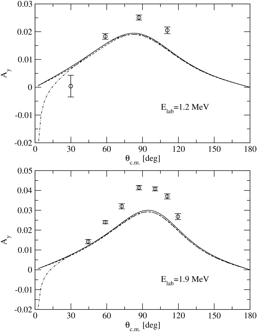
FIG. 1.: The $n-d$ $A_{y}$ calculated using AV18 (solid line) and AV18+MM (dotted-dashed line). For the dashed line see text. Experimental points are from Ref.[20].

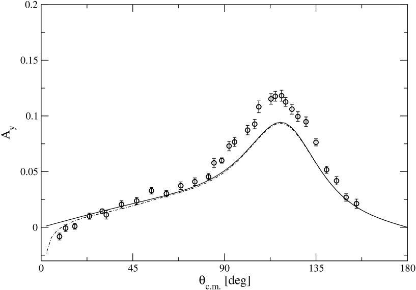
FIG. 2.: The $n-d$ $A_{y}$ at $E_{lab}=6.5$ MeV calculated using AV18 (solid line) and AV18+MM (dotted-dashed line). Experimental points are from Ref.[21].

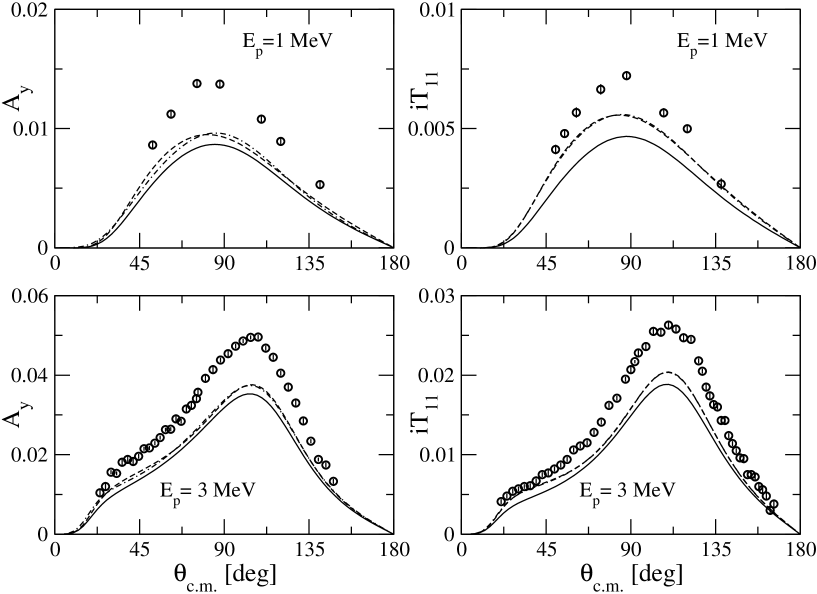
FIG. 3.: The $p-d$ $A_{y}$ and $iT_{11}$ calculated using AV18 (solid line) and AV18+MM (dotted-dashed line). For the dashed line see text. Experimental points are from Ref.[23] ($1$ MeV) and Ref.[25] ($3$ MeV).

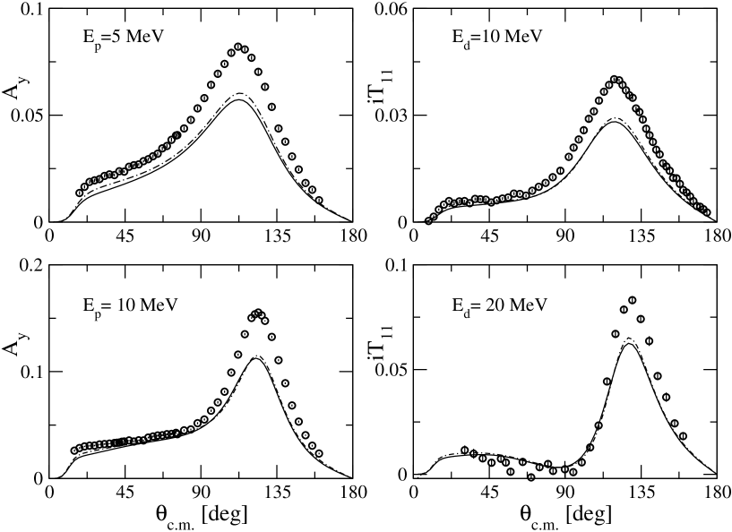
FIG. 4.: The $p-d$ $A_{y}$ and $iT_{11}$ calculated using AV18 (solid line) and AV18+MM (dotted-dashed line). Experimental points at $E_{p}=5,10$ MeV and $E_{d}=10$ MeV are from Ref.[27], $E_{d}=20$ MeV are from Ref.[28].

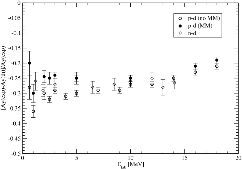
FIG. 5.: Relative difference between the theoretical and experimental vector analyzing power $A_{y}$ at the peak as a function of energy.

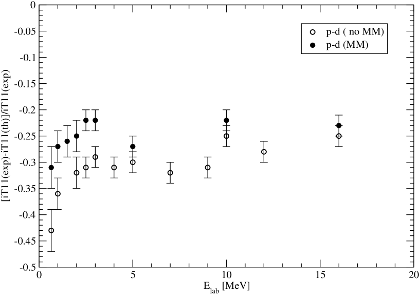
FIG. 6.: Relative difference between the theoretical and experimental vector analyzing power $iT_{11}$ at the peak as a function of energy.

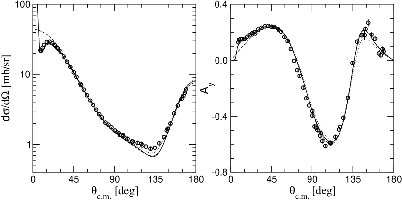
FIG. 7.: The differential cross section and $A_{y}$ at $E_{lab}=65$ MeV. For explanation of the curves see text. Experimental data are from Ref. [29].

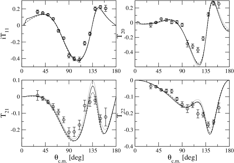
FIG. 8.: The deuteron analyzing power $iT_{11}$ and the tensor analyzing powers $T_{20},T_{21},T_{22}$ at $E_{lab}=65$ MeV. For explanation of the curves see text. Experimental data are from Ref. [30].

REFERENCES

• [1] L.D. Knutson and D. Chiang, Phys. Rev. C18, 1958 (1978)
• [2] V.G.J. Stoks and J.J. de Swart, Phys. Rev. C42, 1235 (1990)
• [3] A. Kievsky, M. Viviani, and S. Rosati, Phys. Rev. C64, 024002 (2001)
• [4] M. Viviani, A. Kievsky, and S. Rosati, Few-Body Syst. 30, 39 (2001)
• [5] A. Kievsky, M. Viviani, and S. Rosati, Nucl. Phys. A577 , 511 (1994)
• [6] A. Kievsky, M. Viviani, and S. Rosati, Nucl. Phys. A551, 241 (1993)
• [7] A. Kievsky, S. Rosati, W. Tornow, and M. Viviani, Nucl. Phys. A607, 402 (1996)
• [8] W. GlΓΆckle et al., Phys. Rep. 274, 107 (1996)
• [9] H. WitaΕ‚a et al., Phys. Rev. C63, 024007 (2001)
• [10] R.B. Wiringa, V.G.J. Stoks, and R. Schiavilla, Phys. Rev. C51, 38 (1995)
• [11] Steven C. Pieper, V.R. Pandharipande, R.B. Wiringa, and J. Carlson, Phys. Rev. C64, 014001 (2001)
• [12] A. Nogga et al., Phys. Rev. C67, 034004 (2003)
• [13] V.G.J. Stoks, Phys. Rev. C57, 445 (1998)
• [14] A. Kievsky, M. Viviani, L.E. Marcucci, and S. Rosati, Few-Body Syst. Suppl. 14, 111 (2003)
• [15] H. WitaΕ‚a et al., Phys. Rev. C67, 064002 (2003)
• [16] L.C. Biedenharn and C.M. Class, Phys. Rev. 98, 691 (1955)
• [17] L.D. Knutson (private communication)
• [18] A. Kievsky, Nucl. Phys. A624, 125 (1997)
• [19] R.G. Seyler, Nucl. Phys. A124, 253 (1969)
• [20] E.M. Neidel et al., Phys. Lett. B552, 29 (2003)
• [21] W. Tornow et al., Phys. Lett. B257, 273 (1991)
• [22] C.R. Brune et al., Phys. Rev. C63, 044013 (2001)
• [23] M.H. Wood et al., Phys. Rev. C65, 034002 (2002)
• [24] L.D. Knutson, L.O. Lamm, and J.E. McAninch, Phys. Rev. Lett.71, 3762 (1993)
• [25] S. Shimizu et al., Phys. Rev. C52, 1193 (1995)
• [26] A. Kievsky et al., Phys. Rev. C63, 024005 (2001)
• [27] K. Sagara et al., Phys. Rev. C50, 576 (1994); K. Sagara (private communication)
• [28] W. GrΓΌebler et al., Nucl. Phys. A398, 445 (1983); F. Sperisen et al., ibid. A422, 81 (1984)
• [29] H. Shimizu et al., Nucl. Phys. A382, 242 (1982)
• [30] H. Witala et al., Few-Body Syst. 15, 67 (1993)
• [31] B.S. Pudliner et al., Phys. Rev. Lett. 74, 4396 (1995)
• [32] J. Carlson and R. Schiavilla, Rev. Mod. Phys. 70, 743 (1998)
• [33] R.G. Arnold, C.E. Carlson, and F. Gross, Phys. Rev. C21, 1426 (1980)
• [34] G.J.M. Austen and J.J. de Swart, Phys. Rev. Lett. 50, 2039 (1983)
• [35] J.L. Forest, V.R. Pandharipande, and J.L. Friar, Phys. Rev. C52, 568 (1995)
Refer to caption