Description of $\eta$-distributions at RHIC energies
in terms of a stochastic model

Abstract

To explain $\eta$-distributions at RHIC energies we consider the Ornstein-Uhlenbeck process. To account for hadrons produced in the central region, we assume existence of third source located there ($y\approx 0$) in addition to two sources located at the beam and target rapidities ($\pm y_{\rm max}=\pm\ln\left[\sqrt{s_{\tiny NN}}/m_{\tiny N}\right]$). This results in better $\chi^{2}/$n.d.f. than those for only two sources when analysing data.

We are interested in analyses of $\eta$-distributions [1, 2] at RHIC energies by means of stochastic process, in particular the Ornstein-Uhlenbeck (O-U) process.[3, 4] Our previous formulation was a simplified approach, because we have sought an empirical formula. Through those studies, we have found that 1) $\eta$-distributions should be a sum of two or more Gaussian distributions, and 2) a $z_{r}=\eta/\eta_{\rm rms}$ scaling holds among various centrality cuts. We have used the following Fokker-Planck equation

$$\frac{\partial P(y,\,t)}{\partial t}=\gamma\left[\frac{\partial[yP(y,\,t)]}{\partial y}+\frac{1}{2}\frac{\sigma^{2}}{\gamma}\frac{\partial^{2}P(y,\,t)}{\partial y^{2}}\right]\,,$$ (1)

where $y$, $\gamma$ and $\sigma^{2}$ are the rapidity, the frictional coefficient and the variance, respectively. The solution with the initial condition $P(y,\,0)=0.5[\delta(y+y_{\rm max})+\delta(y-y_{\rm max})]$ is given as

$$P(y,\,y_{\rm max},\,t) = \frac{1}{\sqrt{8\pi V^{2}(t)}}\left\{\exp\left[-\frac{(y+y_{\rm max}e^{-\gamma t})^{2}}{2V^{2}(t)}\right]\right.$$ (2)

$$\qquad\qquad\quad\left.+\exp\left[-\frac{(y-y_{\rm max}e^{-\gamma t})^{2}}{2V^{2}(t)}\right]\,\right\}\,,$$

where $V_{1}^{2}(t)=(\sigma^{2}/2\gamma)p$ with $p=(1-e^{-2\gamma t})$. See Refs. Wolschin:1999jy and Morita:2002av.

In this paper we investigate a more realistic formulation, namely we take into account the contribution from the central region at $y\approx 0$.[7] For our aim, first of all, we adopt the two-step processes by O-U process shown in Fig. 1.

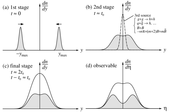
Figure 1: Description of two-step processes by O-U process.

For the third source we assume the following $y$ distribution

$$P_{0}(y,\>t)=\frac{1}{\sqrt{2\pi V_{0}^{2}(t)}}\exp\left[-\frac{y^{2}}{2V_{0}^{2}(t)}\right]\>,$$ (3)

where $P_{0}(y,\,0)=\delta(y)$ and $V_{0}^{2}(t)=(\sigma_{0}/2\gamma)p$. According to the physical picture mentioned above we have therefore following formula for the normalized distribution ($\int dn/d\eta\cdot d\eta=1$) in the $\eta$-rapidity space,

$$\frac{dn}{d\eta}=J(\eta,\>m/p_{t})\times r_{f}\times{\rm Eq.\ (\ref{eq2})}+J_{0}\times(1-r_{f})\times{\rm Eq.\ (\ref{eq3})}\,,$$ (4)

with

$$y=\frac{1}{2}\ln\left\{\left[\sqrt{1+(m/p_{t})^{2}+\sinh^{2}\eta}+\sinh\eta\right]/\left[\sqrt{1+(m/p_{t})^{2}+\sinh^{2}\eta}-\sinh\eta\right]\right\}\>,$$

where the Jacobian factor $J(\eta,\>m/p_{t})=\cosh\eta/\sqrt{1+(m/p_{t})^{2}+\sinh^{2}\eta}$ and $J_{0}=J(\eta,\>m_{0}/p_{t})$. $r_{f}$ is the ratio of the weight factors among the two sources ($c_{1}$) at $\pm y_{\rm max}$ and the third one ($c_{0}$); $r_{f}=2c_{1}/(2c_{1}+c_{0})$.

In concrete analyses, the masses of hadrons in the beam and target nuclei should be larger than those of the central region, because of the richness of baryons; $(m/p_{t})>(m_{0}/p_{t})$, $(m/p_{t})>\delta(m/p_{t})$, $(m_{0}/p_{t})>\delta(m_{0}/p_{t})$. The evolution parameter $p$ is determined at the minimum values of $\chi^{2}$’s, as in the previous treatments.[3, 4]

Our analyses of data by PHOBOS Collaboration [1] at $\sqrt{s_{\tiny NN}}=130$ GeV and $200$ GeV are shown in Fig. 2 and Table 1. As one can see there, a reasonable set of weights, which satisfy our criteria, is $c_{1}/2:c_{0}:c_{1}/2=1:6:1\sim 1:10:1$.

Figure 2: (a) $c_{1}/2:c_{0}:c_{1}/2=1:7:1$, $p=0.73\pm 0.03$, $V_{0}^{2}=4.42\pm 0.84$, $V_{1}^{2}=1.17\pm 0.17$, (b) $c_{1}/2:c_{0}:c_{1}/2=1:7:1$, $p=0.74\pm 0.33$, $V_{0}^{2}=5.19\pm 1.24$, $V_{1}^{2}=1.36\pm 0.23$.

Table 1: Weights ($c_{1}/2:c_{0}:c_{1}/2=1:c_{0}^{\prime}:1$) dependence of $\chi^{2}$’s values.

	$c_{0}^{\prime}$	2	4	6	7	8	10
PHOBOS	$m_{0}/p_{t}$	0.29$\pm$0.91	0.33$\pm$0.56	0.46$\pm$0.11	0.51$\pm$0.28	0.55$\pm$0.25	0.63$\pm$0.20
130 GeV	$m/p_{t}$	0.55$\pm$0.18	0.54$\pm$0.20	0.68$\pm$0.15	0.72$\pm$0.20	0.76$\pm$0.21	0.83$\pm$0.22
0-6 %	$\chi^{2}/$n.d.f.	0.79/47	0.71/47	0.64/47	0.62/47	0.62/47	0.65/47
PHOBOS	$m/p_{t}$	0.22$\pm$1.02	0.36$\pm$0.47	0.47$\pm$0.34	0.51$\pm$0.29	0.55$\pm$0.27	0.61$\pm$0.23
200 GeV	$m/p_{t}$	0.45$\pm$0.16	0.54$\pm$0.24	0.69$\pm$0.28	0.58$\pm$0.26	0.62$\pm$0.24	0.69$\pm$0.33
0-6 %	$\chi^{2}/$n.d.f.	0.63/47	0.68/47	0.76/47	0.81/47	0.88/47	1.02/47

Moreover, to confirm the $z_{r}=\eta/\eta_{\rm rms}$ ($\eta_{\rm rms}=\sqrt{\langle\eta^{2}\rangle}$) scaling we compare our theoretical formula

$$\eta_{\rm rms}\frac{dn}{d\eta}=\frac{dn}{dz_{r}}=\eta_{\rm rms}\times{\rm Eq.\ (\ref{eq4})}|_{\eta=z_{r}\eta_{\rm rms}}$$ (5)

with data including 5 centrality cuts. Explanations of the $z_{r}$ scaling by means of Eq. (5) shown in Fig. 3 seem to be excellent.

Figure 3: $z_{r}$ scaling by Eq. (5). (a) $\chi^{2}/{\rm n.d.f.}=21.2/318$. (b) $\chi^{2}/{\rm n.d.f.}=11.5/318$. Dotted lines mean the error bars.

Hereafter, we analyzed data by BRAHMS Collaboration [2] at 200 GeV using Eqs. (4) and (5). In this case our criterion mentioned above cannot be applied, as seen in Table 2, because of fluctuation in $dn/d\eta$ and restricted data points in fragmentation regions. Therefore we have assumed the evolution parameter $p=0.75$ taken from Fig. 2(b) which results in reasonable value of $\chi^{2}$’s at $c_{1}/2:c_{0}:c_{1}/2=1:20:1$. The $z_{r}$ scaling shown in Fig. 4 holds with $c_{1}/2:c_{0}:c_{1}/2=1:10:1$ in a sense of the averaged centrality cuts.

Table 2: Same as Table 1 but data by BRAHMS Collaboration at 200 GeV.

		$p=$ free			$p=0.75$ (fixed)
	$c_{0}^{\prime}$	5	10	20	5	10	20
BRAHMS	$m_{0}/p_{t}$	0.57$\pm$0.33	0.51$\pm$0.18	0.56$\pm$0.16	0.29$\pm$0.38	0.37$\pm$0.46	0.55$\pm$0.24
200 GeV	$m/p_{t}$	6.2$\pm$2.9	7.1$\pm$2.7	16.7$\pm$25.0	0.00$\pm$2.15	0.35$\pm$1.57	0.78$\pm$0.66
0-5 %	$p$	1.00$\pm$0.80	1.00$\pm$0.84	1.00$\pm$0.03	0.75	0.75	0.75
	$\chi^{2}/$n.d.f.	4.70/30	4.56/30	3.89/30	4.94/31	4.70/31	4.37/31

Figure 4: (a) $c_{1}/2:c_{0}:c_{1}/2=1:20:1$, $\chi^{2}=4.68/30$, $y_{max}=5.36$ (fixed), $p=0.75$ (fixed), $V_{0}^{2}=6.42\pm 0.95$, $V_{1}^{2}=0.79\pm 0.23$. (b) $z_{r}$ scaling, $c_{1}/2:c_{0}:c_{1}/2=1:10:1$, $p=0.95\pm 0.06$, $\chi^{2}/{\rm n.d.f.}=29.8/186$. Dotted lines mean the error bars.

In conclusion, the two-step processes by O-U process is available for the description of $\eta$-distributions at RHIC energies.

Acknowledgements: One of authors (M. B.) would like to thank the Scandinavia-Japan Sasakawa Foundation for financial support, 2002. In addition this study is partially supported by a research program of Shinshu University, 2002. They are indebted to G. Wilk for his reading the manuscript. Moreover, we would like to appreciate various conversations at International Workshop ”Finite Density QCD” held in Nara.

References

• [1] B. B. Back et al. [PHOBOS Collaboration], Phys. Rev. Lett.  87 (2001), 102303; R. Nouicer et al. [PHOBOS Collaboration], nucl-ex/0208003.
• [2] I. G. Bearden et al. [BRAHMS Collaborations], Phys. Lett. B 523 (2001), 227; Phys. Rev. Lett. 88 (2002), 202301.
• [3] M. Biyajima, M. Ide, T. Mizoguchi and N. Suzuki, Prog. Theor. Phys.  108 (2002), 559 [Addendum-ibid.  109 (2003), 151]. See also, M. Biyajima, Phys. Lett. B 139 (1984), 93, and M. Biyajima et al., Phys. Lett. B 515 (2001), 470.
• [4] M. Biyajima and T. Mizoguchi, Prog. Theor. Phys.  109 (2003), 483; M. Ide, M. Biyajima and T. Mizoguchi, arXiv:nucl-th/0302003.
• [5] G. Wolschin, Eur. Phys. J. A 5 (1999), 85:
• [6] K. Morita, S. Muroya, C. Nonaka and T. Hirano, Phys. Rev. C 66 (2002), 054904.
• [7] G. Wolschin, Phys. Lett. B 569 (2003), 67; therein the fractional Fokker-Planck equation is assumed for the central region; See also M. Rybczynski, Z. Wlodarczyk and G. Wilk, Nucl. Phys. Proc. Suppl.  122 (2003), 325 [arXiv:hep-ph/0206157].