Hadronic Effective Field Theory Applied to $\Lambda$-Hypernuclei

Abstract

In the present work, the approach of Furnstahl, Serot, and Tang (FST) is extended to the region of nonzero strangeness in application to single-particle states in single $\Lambda$-hypernuclei. To include $\Lambda$’s, an additional contribution to their effective lagrangian is systematically constructed within the framework of FST. The relativistic Hartree (Kohn-Sham) equations are solved numerically, and least-square fits to a series of experimental levels are performed at various levels of truncation in the extended lagrangian. The ground-state properties of any $\Lambda$-hypernuclei are then predicted. In addition, ground-state $\Lambda$-particle–nucleon-hole splittings are calculated where appropriate, and the approach is calibrated against a calculation of the $\mathrm{s}_{1/2}$-doublet splitting in the nucleus ${}^{32}_{15}\mathrm{P}_{17}$.

21.80.+a

1 Introduction

Effective field theories have been developed in recent years to solve the nuclear many-body problem. In the present work, we consider one of these theories, proposed by Furnstahl, Serot, and Tang (FST) [1, 2], and extend their methodology to the case of single $\Lambda$-hypernuclei. Specifically, the phenomena of interest here are ground-state (GS) binding energies, densities, single-particle spectra, and particle-hole splittings of select single $\Lambda$-hypernuclei.

FST develop a self-consistent framework for constructing an effective lagrangian that incorporates the principles of both quantum mechanics and special relativity, the underlying symmetries of QCD, and the nonlinear realization of spontaneously broken chiral symmetry [1]. As this is a low-energy theory, the appropriate low lying hadrons are used as degrees of freedom. In order to make any meaningful calculation, the lagrangian, which in principle contains an infinite number of terms, must be truncated in some way. Naive dimensional analysis (NDA) [3, 4] and relativistic mean field theory (RMFT) [2, 5] provide a formalism in which higher order terms are, in general, successively smaller; this allows for a systematic expansion, and consequently a meaningful truncation, in the effective lagrangian. Here FST utilize relativistic Hartree theory to reduce the many-body equations to single-particle equations. The free parameters in the effective lagrangian are fixed via least-squares fits to experimental data from ordinary nuclei along the valley of stability. These fits are conducted at various levels of truncation in the underlying lagrangian [1]. Once the values of these parameters are known, this lagrangian can be used to predict other properties of ordinary nuclei. One example which demonstrates the predictive power of this method is its application to the study of nuclei far from stability [6, 7].

Density functional theory (DFT) is a theoretical framework which allows one to calculate the GS properties of many-body systems without carrying around all the baggage contained in the many-particle wave functions [8]. Two points are of interest here. First, if the expectation value of the hamiltonian is considered as a functional of the density, the exact GS density can be determined by minimizing the energy functional. Second, one only needs to solve a series of self-consistent, single-particle equations with classical fields, instead of many-body equations with quantum fields [9]. In other words, Kohn-Sham theory is formally equivalent to relativistic Hartree theory. Consequently, the problem is now reduced to determining the correct form of the energy functional, which follows from the appropriate lagrangian. The full interacting lagrangian of FST gives an appropriate energy functional and, as a result, DFT provides an underlying theoretical justification for this approach.

Hadronic effective lagrangians using MFT have been developed in the literature to describe hypernuclei. Early models containing only the lowest order terms required much weaker meson couplings to the $\Lambda$ than to the nucleons to achieve success [10, 11], particularly in the weak spin-orbit interaction. Later, it was suggested that large meson couplings to the $\Lambda$ consistent with $\mathrm{SU(3)}$ were possible if the lagrangian was extended to include tensor couplings [12, 13, 14, 15, 16, 17, 18]. It turns out the spin-orbit splitting is very sensitive to the size of the tensor coupling to the vector field. The approach of FST has also been applied to strange hadronic matter [19]. More recently, effective theories consistent with $\mathrm{SU(3)_{L}\otimes SU(3)_{R}}$ have been constructed [20, 21, 22]. Another model of interest uses strangeness changing response functions to calculate the spectra of $\mathrm{{}^{16}_{Y}O}$ and $\mathrm{{}^{40}_{Y}Ca}$; the resulting GS particle-hole splittings are small [23]. Other studies include models that couple the mesons self-consistently to the quarks within the baryons [24, 25] and a density dependent relativistic hadronic field theory [26].

The following studies have attempted to fit potentials to the hyperon-nucleon interaction. Experimental data has been analyzed to obtain a nonlocal and density-dependent $\Lambda$-nucleus potential [27, 28]. Global optical potentials for $\Lambda$ scattering off nuclei were developed [29]. The hypernuclear mass dependence of the binding energies is reproduced by a $\Lambda$ moving in a Woods-Saxon potential [30]. The Nijmegen group has developed Y-N potentials based on the assumption of $\mathrm{SU(3)}$ symmetry [31, 32, 33]; this fixes the baryon-meson coupling constants from N-N scattering fits. Similarly, potentials were constructed by the Julich group assuming $\mathrm{SU(6)}$ symmetry [34]. Calculations of hypernuclei using these Nijmegen or Julich potentials include [35, 36, 37, 38, 39, 40]. Comparable G-matrix calculations with a $\mathrm{SU(6)}$ quark-model baryon-baryon interaction [41] and Skyrme-like hyperon-nucleon potentials [42] have also been investigated. Other recent approaches include using the Fermi hypernetted chain method [43, 44] and using a quark model with one boson exchange potentials [45].

Many of these studies achieve a good deal of success. However, the framework of FST is more comprehensive than these approaches as it incorporates directly into a hadronic effective field theory all of the following: special relativity, quantum mechanics, the underlying symmetry structure of QCD, and the nonlinear realization of spontaneously broken chiral symmetry. Furthermore, this methodology is theoretically justified by DFT. Once all the parameters are fixed, their lagrangian predicts the GS properties of any ordinary nucleus. This approach has had great success [1, 6, 7]. Therefore, it is of interest to extend this methodology, with all of its intrinsic strengths, to the strangeness sector, as is done here.

In the present work, the approach developed by FST is expanded to the region of the strangeness sector that corresponds to $\Lambda$-hypernuclei with $\mathrm{S=-1}$ and $\mathrm{T=0}$. To this end, we include a single, isoscalar $\Lambda$ field in the theory. Now, a $\Lambda$-lagrangian is constructed as an additional contribution to the full interacting effective lagrangian of FST, consistent with their methodology. Since the $\Lambda$ is an isoscalar, it does not couple to either a single Yukawa pion or the rho meson. Furthermore, we confine our theory to the mesons already included; thus, the meson lagrangian, which in this approach contains the majority of the complexity, is unaltered. It has been proposed that a tensor coupling to the vector field be included to reproduce the correct experimental spin-orbit splitting of the p-states in $\Lambda$-hypernuclei [12, 13]. As it turns out, such a term is a natural extension of our lagrangian in this framework. Additional higher order terms are also included to better approximate the exact energy functional.

Following the methodology of FST, our $\Lambda$-lagrangian contains a number of free parameters. The constants in both the nucleon and meson sectors are taken from a FST parameter set corresponding to their full lagrangian. As before, the remaining unconstrained parameters are fixed here via least-squares fits to a series of experimental data [47, 48, 49, 50, 51, 52]. The 10 pieces of data used include six GS binding energies, three s-p shell excitations for the $\Lambda$, and the spin-orbit splitting of the p-states in ${}^{13}_{\Lambda}\mathrm{C}$. The fits are conducted at four different levels of truncation in the $\Lambda$-lagrangian. Once these parameters are fixed, this lagrangian can be used to predict other properties of single $\Lambda$-hypernuclei.

One other property that is of interest to calculate here is what we refer to as $\mathrm{s}_{1/2}$-splittings. These are GS particle-hole splittings of select single $\Lambda$-hypernuclei, such as ${}^{16}_{\Lambda}\mathrm{O}$, which have a $\Lambda$ in the GS and a hole in the last filled nucleon (proton or neutron) shell. For these systems, the angular momenta of the $\Lambda$ and the nucleon hole couple to form a doublet. The size of these splittings is determined by the difference of two particle-hole matrix elements [53]. The effective particle-hole interaction utilized here follows directly from the effective theory of the preceding discussion. This interaction, to lowest order, is just simple scalar and vector meson exchange [54]. A simple Yukawa spatial dependence is obtained when retardation is neglected in the meson propagators. With this exception, the full Lorentz structure is maintained [54]. For the $\Lambda$-N case, there is no isovector component to the effective interaction or exchange contribution in the two-body matrix elements. Through angular momentum relations [57] and some algebra, the matrix elements are reduced to radial Slater integrals. Using the Hartree wave functions from the $\Lambda$ single-particle calculations to evaluate the integrals, these matrix elements, and consequently the $\mathrm{s_{1/2}}$-splitting, can now be fully determined. Once the parameters in the $\Lambda$-lagrangian are known, the effective particle-hole interaction is completely specified in this approach. In the case of $\mathrm{s_{1/2}}$-splittings in $\Lambda$-hypernuclei, only the spatial part of the vector exchange contributes to the splitting. Predictions are given for the GS doublet splittings of every one of the $\Lambda$-hypernuclei considered here; all of the doublets used in the fitting procedure lie within the current experimental error bars on the GS energies. An upcoming high resolution experiment at Jefferson Lab will measure the $\mathrm{s_{1/2}}$-splittings in ${}^{12}_{\Lambda}\mathrm{B}$ and ${}^{16}_{\Lambda}\mathrm{N}$ [58, 59]. The present calculations provide theoretical predictions for these quantities.${}^{\ref{foot:1}}$ Non-relativistic calculations of similar particle-hole splittings have been carried out [60].

The need for isovector interactions and exchange contributions make calculations of similar splittings in ordinary nuclei far more complicated [54]. As an example of a comparable system in an ordinary nucleus, and to at least partially calibrate the present approach, the calculation of the $\mathrm{s_{1/2}}$-splitting in ${}^{32}_{15}\mathrm{P}_{17}$ is included here. Comparable systems for ordinary nuclei have also been examined [61].

In section 2, we review the methodology of FST and in section 3, we describe the development of our $\Lambda$-lagrangian. The framework for calculating the particle-hole splittings is discussed in section 4. The results of the parameter fits, single-particle calculations, and $\mathrm{s_{1/2}}$-splittings are given in section 5.

2 Methodology of FST

In this section we review the methodology of FST. They approach the nuclear many-body problem by constructing an effective field theory that retains the underlying symmetries of QCD as well as the principles of both special relativity and quantum mechanics [1]. At low-energy, hadrons are the desired degrees of freedom and the ones which FST use to construct an effective lagrangian. The nonlinear realization of spontaneously broken chiral symmetry is illustrated through a system of pions, nucleons, and rho mesons. They incorporate Goldstone pions through the field

$$\mathrm{U(x_{\mu})\equiv\xi(x_{\mu})\mathbf{1}\xi(x_{\mu})}=e^{i\pi(\mathrm{x_{\mu}})/f_{\pi}}\mathbf{1}e^{i\pi(\mathrm{x_{\mu}})/f_{\pi}}$$ (1)

where the pion field, $\pi(\mathrm{x_{\mu}})=\frac{1}{2}\vec{\tau}\cdot\vec{\pi}$, appears to all orders, $\tau$ is a Pauli matrix, and $f_{\pi}$ is the pion-decay constant [1]. An isodoublet nucleon field is included, represented by

$$\mathrm{N(x_{\mu})}=\left(\begin{array}[]{c}\mathrm{p(x_{\mu})}\\ \mathrm{n(x_{\mu})}\end{array}\right)$$ (2)

The upper (lower) component corresponds to the proton (neutron). To account for the symmetry energy in nuclear matter, an isovector-vector rho meson, $\rho_{\nu}(\mathrm{x_{\mu}})=\frac{1}{2}\vec{\tau}\cdot\vec{\rho}$, is also included.

The following boson fields are also incorporated into this framework, the first two of which are isoscalar chiral singlets. A scalar field, $\phi$, is included to simulate the medium-range nuclear attraction. Next, they incorporate a vector meson, $\mathrm{V_{\mu}}$, to reproduce the short-range nuclear repulsion. Lastly, a photon field, $\mathrm{A_{\mu}}$, is added to take into consideration the electromagnetic structure of nuclei.

As all possible combinations of the fields, consistent with this framework, are included, this lagrangian contains an infinite number of terms. To conduct any meaningful calculation, this lagrangian needs to be truncated at some level. FST utilize both NDA and RMFT to accomplish this. NDA is a framework which identifies all the dimensional factors of a given term. Once these dimensional factors, and some appropriate counting factors, are extracted from a term, the remaining dimensionless constant is of $O(1)$ [3, 4]. This assumption is known as “naturalness.” RMFT states that when the baryon density becomes appropriately large, the sources and meson fields can be replaced by their expectation values; here, the expectation values of the meson fields are just their classical fields [5]. Then we notice that while the meson mean fields are large, the ratios of these fields to the chiral symmetry breaking scale, M, are small. Furthermore, the size of derivatives is related to $k_{\mathrm{F}}$, which is also small compared to M. These effects are shown by [5]

$$\mathrm{\frac{\Phi}{M}\;,\;\frac{W}{M}}\sim\frac{1}{3};\;\;\;\;\;\;\;\;\;\;\;\;\;\frac{k_{\mathrm{F}}}{\mathrm{M}}\sim\frac{1}{4}$$ (3)

where the scaled meson mean fields are defined as

$$\Phi(\vec{\mathrm{x}})\equiv\mathrm{g_{S}\phi_{0};}\;\;\;\;\;\;\mathrm{W}(\vec{\mathrm{x}})\equiv\mathrm{g_{V}V_{0};}\;\;\;\;\;\;\mathrm{R}(\vec{\mathrm{x}})\equiv\mathrm{g_{\rho}b_{0};}\;\;\;\;\;\;\mathrm{A}(\vec{\mathrm{x}})\equiv\mathrm{eA_{0}}$$ (4)

The ordering principle developed by FST is

$$\nu=\frac{n}{2}+b+d$$ (5)

where for a given term $\nu$ is the order, $n$ is the number of fermion fields, $b$ is the number of non-Goldstone bosons, and $d$ is the number of derivatives. Now a controlled expansion is performed in which higher order terms are, in general, progressively smaller.

Using this ordering principle, they construct an effective lagrangian in two parts [1]

$$\mathrm{{\cal{L}}_{FST}(x_{\mu})={\cal{L}}_{N}(x_{\mu})+{\cal{L}}_{M}(x_{\mu})}$$ (6)

The fermion part to order $\nu=4$ is given by

$$\mathrm{{\cal{L}}_{N}(x_{\mu})} = -\bar{\mathrm{N}}\left\{\gamma_{\mu}\left[\frac{\partial}{\partial\mathrm{x_{\mu}}}+iv_{\mu}-i\mathrm{g_{A}}\gamma_{5}a_{\mu}-i\mathrm{g_{V}V_{\mu}}-i\mathrm{g}_{\rho}\rho_{\mu}\right.\right.$$ (7)

$$- \left.\left.\frac{i}{2}\mathrm{eA_{\mu}}\left(1+\tau_{3}\right)\right]+\mathrm{\left(M-g_{S}\phi\right)}\right\}\mathrm{N}+\frac{f_{\rho}\mathrm{g}_{\rho}}{\mathrm{4M}}\mathrm{\bar{N}\sigma_{\mu\nu}\rho_{\mu\nu}N}$$

$$+ \frac{f\mathrm{{}_{V}g_{V}}}{\mathrm{4M}}\mathrm{\bar{N}\sigma_{\mu\nu}V_{\mu\nu}N}+\mathrm{\frac{\kappa_{\pi}}{M}\bar{N}}\sigma_{\mu\nu}v_{\mu\nu}\mathrm{N}+\mathrm{\frac{e}{4M}\bar{N}\lambda\sigma_{\mu\nu}F_{\mu\nu}N}$$

$$+ \frac{i\mathrm{e}}{\mathrm{2M^{2}}}\mathrm{\bar{N}\gamma_{\mu}\left(\beta_{S}+\beta_{V}\tau_{3}\right)N\frac{\partial}{\partial x_{\nu}}F_{\mu\nu}}$$

where $\lambda=\frac{1}{2}\lambda_{\mathrm{p}}(1+\tau_{3})+\frac{1}{2}\lambda_{\mathrm{n}}(1-\tau_{3})$ and $\lambda_{\mathrm{p}}=1.793$ ($\lambda_{\mathrm{n}}=-1.913$) is the anomalous magnetic moment of the proton (neutron). Note that for the purposes of this work, the conventions of [5] are used. Here we have defined

$$\mathrm{V_{\mu\nu}=\frac{\partial V_{\nu}}{\partial x_{\mu}}-\frac{\partial V_{\mu}}{\partial x_{\nu}}}$$ (8)

$v_{\mu\nu}$, $\rho_{\mu\nu}$, and $\mathrm{F}_{\mu\nu}$ are similarly defined for $v_{\mu}$, $\rho_{\mu}$, and $\mathrm{A}_{\mu}$ respectively. Notice that the pions only couple to the fermions through the combinations

$$v_{\mu}=-\frac{i}{2}\left(\xi^{\dagger}\frac{\partial\xi}{\partial\mathrm{x}_{\mu}}+\xi\frac{\partial\xi^{\dagger}}{\partial\mathrm{x}_{\mu}}\right)=v_{\mu}^{\dagger}$$ (9)

$$a_{\mu}=\frac{i}{2}\left(\xi^{\dagger}\frac{\partial\xi}{\partial\mathrm{x}_{\mu}}-\xi\frac{\partial\xi^{\dagger}}{\partial\mathrm{x}_{\mu}}\right)=a_{\mu}^{\dagger}$$ (10)

To lowest order, both $v_{\mu}$ and $a_{\mu}$ contain derivatives of the pion field; thus soft pions decouple. The meson lagrangian to order $\nu=4$ is

$$\mathrm{{\cal{L}}_{M}(x_{\mu})} = \mathrm{-\frac{1}{2}\left(1+\alpha_{1}\frac{g_{S}\phi}{M}\right)\left(\frac{\partial\phi}{\partial x_{\mu}}\right)^{2}}-\frac{f_{\pi}^{2}}{4}\mathrm{tr\left(\frac{\partial U}{\partial x_{\mu}}\frac{\partial U^{\dagger}}{\partial x_{\mu}}\right)}-\frac{1}{2}\mathrm{tr}\left(\rho_{\mu\nu}\rho_{\mu\nu}\right)$$ (11)

$$- \mathrm{\frac{1}{4}\left(1+\alpha_{2}\frac{g_{S}\phi}{M}\right)V_{\mu\nu}V_{\mu\nu}}-\mathrm{g}_{\rho\pi\pi}\frac{2f_{\pi}^{2}}{\mathrm{m}_{\rho}^{2}}\mathrm{tr}\left(\rho_{\mu\nu}v_{\mu\nu}\right)$$

$$+ \frac{\mathrm{m_{\pi}^{2}}f_{\pi}^{2}}{4}\mathrm{tr\left(U+U^{\dagger}-2\right)}-\mathrm{\frac{1}{2}\left(1+\eta_{1}\frac{g_{S}\phi}{M}+\frac{\eta_{2}}{2}\frac{g_{S}^{2}\phi^{2}}{M^{2}}\right)m_{V}^{2}V_{\mu}V_{\mu}}$$

$$+ \mathrm{\frac{1}{4!}\zeta_{0}g_{V}^{2}\left(V_{\mu}V_{\mu}\right)^{2}-\frac{1}{4}F_{\mu\nu}F_{\mu\nu}}-\mathrm{\left(1+\eta_{\rho}\frac{g_{S}\phi}{M}\right)m_{\rho}^{2}tr\left(\rho_{\mu}\rho_{\mu}\right)}$$

$$- \mathrm{m_{S}^{2}\phi^{2}\left(\frac{1}{2}+\frac{\kappa_{3}}{3!}\frac{g_{S}\phi}{M}+\frac{\kappa_{4}}{4!}\frac{g_{S}^{2}\phi^{2}}{M^{2}}\right)}$$

Terms such as $\mathrm{\bar{N}N}\phi^{2}$ are redundant in this formulation. This stems from the fact that FST employ meson field redefinitions; since the parameters are free, they are also just redefined. A detailed description of how this lagrangian was constructed is presented in [1].

This still constitutes a system of many-body equations with quantum fields. FST now employ Hartree theory and RMFT to reduce the many-body system to a series of single-particle equations with classical fields. This is equivalent to Kohn-Sham theory in DFT; therefore, DFT provides the theoretical justification for this methodology. The single-particle hamiltonian takes the form [1]

$$\mathrm{h}(\vec{\mathrm{x}}) = -i\vec{\alpha}\cdotp\vec{\nabla}+\mathrm{W+\frac{1}{2}\tau_{3}R+\frac{1}{2}\left(1+\tau_{3}\right)A+\mathrm{\beta\left(M-g_{S}\Phi\right)}}-\frac{i}{\mathrm{2M}}\lambda\beta\vec{\alpha}\cdotp\vec{\nabla}\mathrm{A}$$ (12)

$$- \frac{i}{\mathrm{2M}}\beta\vec{\alpha}\cdotp\left(f_{\mathrm{V}}\vec{\nabla}\mathrm{W}+f_{\rho}\frac{1}{2}\tau_{3}\vec{\nabla}\mathrm{R}\right)+\mathrm{\frac{1}{2M^{2}}\left(\beta_{S}+\beta_{V}\tau_{3}\right)\nabla^{2}A}$$

Since the pion has no mean field in a spherically symmetric system, all of the pion couplings drop out. The Hartree wave functions are of the form

$$\psi_{\alpha}(\vec{\mathrm{x}})=\mathrm{\frac{1}{r}}\left(\begin{array}[]{c}i\mathrm{G}_{a}(\mathrm{r})\Phi_{\kappa\mathrm{m}}\\ -\mathrm{F}_{a}(\mathrm{r})\Phi_{-\kappa\mathrm{m}}\end{array}\right)\zeta_{t}$$ (13)

Here $\mathrm{\alpha=\{a,m\}=\{nlsj,m\}}$, $\zeta_{t}$ is a two component spinor, and $t_{a}$ is 1/2 (-1/2) for protons (neutrons). The $\Phi_{\kappa\mathrm{m}}$ are the spin spherical harmonics. Substituting this wave function into the Dirac equation,

$$\mathrm{h}(\vec{\mathrm{x}})\psi_{\alpha}(\vec{\mathrm{x}})=\mathrm{E}_{a}\psi_{\alpha}(\vec{\mathrm{x}})$$ (14)

one arrives at the following radial Hartree equations

$$\left[\frac{\partial}{\partial\mathrm{r}}+\frac{\kappa}{\mathrm{r}}\right]\mathrm{G}_{a}(\mathrm{r})-\left[\mathrm{E}_{a}-\mathrm{U_{1}+U_{2}}\right]\mathrm{F}_{a}(\mathrm{r})-\mathrm{U_{3}G}_{a}(\mathrm{r})=0$$ (15)

$$\left[\frac{\partial}{\partial\mathrm{r}}-\frac{\kappa}{\mathrm{r}}\right]\mathrm{F}_{a}(\mathrm{r})+\left[\mathrm{E}_{a}-\mathrm{U_{1}-U_{2}}\right]\mathrm{G}_{a}(\mathrm{r})+\mathrm{U_{3}F}_{a}(\mathrm{r})=0$$ (16)

where the single-particle potentials are

$$\mathrm{U_{1}(r)} = \mathrm{W(r)}+t_{a}\mathrm{R(r)}+\left(t_{a}+\frac{1}{2}\right)\mathrm{A(r)}+\mathrm{\frac{1}{2M^{2}}}\left(\beta_{\mathrm{S}}+2t_{a}\beta_{\mathrm{V}}\right)\nabla^{2}\mathrm{A(r)}\>\>\>\>\>\>\>$$ (17)

$$\mathrm{U_{2}(r)} = \mathrm{M-\Phi(r)}$$ (18)

$$\mathrm{U_{3}(r)} = \frac{1}{\mathrm{2M}}\left[f_{\mathrm{V}}\mathrm{\frac{\partial W(r)}{\partial r}}+t_{a}f_{\rho}\mathrm{\frac{\partial R(r)}{\partial r}}\right]$$ (19)

$$+ \mathrm{\frac{1}{2M}\frac{\partial A(r)}{\partial r}}\left[\frac{\left(\mathrm{\lambda_{p}+\lambda_{n}}\right)}{2}+t_{a}(\mathrm{\lambda_{p}-\lambda_{n}})\right]$$

The scalar meson equation is determined by minimizing the variational derivative of the effective lagrangian with respect to the scalar meson field. The other meson equations are constructed in a similar fashion. These meson equations are [1]

$$-\nabla^{2}\Phi+\mathrm{m_{S}^{2}}\Phi = \mathrm{g_{S}^{2}}\rho_{\mathrm{S}}(\vec{\mathrm{x}})-\mathrm{\frac{m_{S}^{2}}{M}\Phi^{2}\left(\frac{\kappa_{3}}{2}+\frac{\kappa_{4}}{3!}\frac{\Phi}{M}\right)}$$ (20)

$$+ \mathrm{\frac{g_{S}^{2}}{2M}\left(\eta_{1}+\eta_{2}\frac{\Phi}{M}\right)\frac{m_{V}^{2}}{g_{V}^{2}}W^{2}}+\mathrm{\frac{\alpha_{1}}{2M}}\left[\left(\vec{\nabla}\Phi\right)^{2}+2\Phi\nabla^{2}\Phi\right]$$

$$+ \mathrm{\frac{\alpha_{2}g_{S}^{2}}{2Mg_{V}^{2}}}\left(\vec{\nabla}\mathrm{W}\right)^{2}+\mathrm{\frac{g_{S}^{2}\eta_{\rho}}{2M}\frac{m_{\rho}^{2}}{g_{\rho}^{2}}R^{2}}$$

$$\mathrm{-\nabla^{2}W+m_{V}^{2}W} = \mathrm{g_{V}^{2}}\left[\mathrm{\rho_{B}}(\vec{\mathrm{x}})+\frac{f_{\mathrm{V}}}{2\mathrm{M}}\vec{\nabla}\cdotp\left(\mathrm{\rho_{B}^{T}}(\vec{\mathrm{x}})\mathrm{\hat{r}}\right)\right]$$ (21)

$$- \mathrm{\left(\eta_{1}+\frac{\eta_{2}}{2}\frac{\Phi}{M}\right)\frac{\Phi}{M}m_{V}^{2}W}-\mathrm{\frac{1}{3!}\zeta_{0}W^{3}}$$

$$+ \mathrm{\frac{\alpha_{2}}{M}}\left(\vec{\nabla}\Phi\cdotp\vec{\nabla}\mathrm{W}+\Phi\nabla^{2}\mathrm{W}\right)-\mathrm{\frac{e^{2}g_{V}}{3g_{\gamma}}}\mathrm{\rho_{chg}}(\vec{\mathrm{x}})$$

$$\mathrm{-\nabla^{2}R+m_{\rho}^{2}R} = \frac{1}{2}\mathrm{g}_{\rho}^{2}\left[\rho_{3}(\vec{\mathrm{x}})+\frac{f_{\rho}}{2\mathrm{M}}\vec{\nabla}\cdotp\left(\mathrm{\rho_{3}^{T}}(\vec{\mathrm{x}})\mathrm{\hat{r}}\right)\right]-\mathrm{\eta_{\rho}\frac{\Phi}{M}m_{\rho}^{2}R}$$ (22)

$$- \mathrm{\frac{e^{2}g_{\rho}}{g_{\gamma}}}\mathrm{\rho_{chg}}(\vec{\mathrm{x}})$$

$$\mathrm{-\nabla^{2}A} = \mathrm{e^{2}}\mathrm{\rho_{chg}}(\vec{\mathrm{x}})$$ (23)

The baryon sources become the densities in the meson equations and are given here by [1]

$$\mathrm{\rho_{S}}(\vec{\mathrm{x}}) = \sum_{a}\frac{2j_{a}+1}{4\pi\mathrm{r}^{2}}\left(\mathrm{G}_{a}^{2}(\mathrm{r})-\mathrm{F}_{a}^{2}(\mathrm{r})\right)$$ (24)

$$\mathrm{\rho_{B}}(\vec{\mathrm{x}}) = \sum_{a}\frac{2j_{a}+1}{4\pi\mathrm{r}^{2}}\left(\mathrm{G}_{a}^{2}(\mathrm{r})+\mathrm{F}_{a}^{2}(\mathrm{r})\right)$$ (25)

$$\mathrm{\rho_{B}^{T}}(\vec{\mathrm{x}}) = \sum_{a}\frac{2j_{a}+1}{4\pi\mathrm{r}^{2}}2\mathrm{G}_{a}(\mathrm{r})\mathrm{F}_{a}(\mathrm{r})$$ (26)

$$\mathrm{\rho_{3}}(\vec{\mathrm{x}}) = \sum_{a}\frac{2j_{a}+1}{4\pi\mathrm{r}^{2}}\left(2t_{a}\right)\left(\mathrm{G}_{a}^{2}(\mathrm{r})+\mathrm{F}_{a}^{2}(\mathrm{r})\right)$$ (27)

$$\mathrm{\rho_{3}^{T}}(\vec{\mathrm{x}}) = \sum_{a}\frac{2j_{a}+1}{4\pi\mathrm{r}^{2}}\left(2t_{a}\right)2\mathrm{G}_{a}(\mathrm{r})\mathrm{F}_{a}(\mathrm{r})$$ (28)

The charge density is made up of two components

$$\mathrm{\rho_{chg}}(\vec{\mathrm{x}})=\mathrm{\rho_{d}}(\vec{\mathrm{x}})+\mathrm{\rho_{m}}(\vec{\mathrm{x}})$$ (29)

where the first, the direct nucleon charge density, is

$$\mathrm{\rho_{d}}(\vec{\mathrm{x}})=\mathrm{\rho_{p}}(\vec{\mathrm{x}})+\frac{1}{2\mathrm{M}}\vec{\nabla}\cdotp\left(\rho_{a}^{\mathrm{T}}(\vec{\mathrm{x}})\mathrm{\hat{r}}\right)+\mathrm{\frac{1}{2M^{2}}\left[\beta_{S}\nabla^{2}\rho_{B}+\beta_{V}\nabla^{2}\rho_{3}\right]}$$ (30)

and the second, the vector meson contribution, is

$$\mathrm{\rho_{m}}(\vec{\mathrm{x}})=\mathrm{\frac{1}{g_{\gamma}g_{\rho}}\nabla^{2}R+\frac{1}{3g_{\gamma}g_{V}}\nabla^{2}W}$$ (31)

The point proton and nucleon tensor densities in Eq. (30) are

$$\mathrm{\rho_{p}}(\vec{\mathrm{x}}) = \frac{1}{2}\sum_{a}\frac{2j_{a}+1}{4\pi\mathrm{r}^{2}}(1+2t_{a})(\mathrm{G}_{a}^{2}\mathrm{(r)}+\mathrm{F}_{a}^{2}(\mathrm{r}))$$ (32)

$$= \frac{1}{2}\left(\rho_{\mathrm{B}}+\rho_{3}\right)$$

$$\rho_{a}^{\mathrm{T}}(\vec{\mathrm{x}}) = \sum_{a}\frac{2j_{a}+1}{4\pi\mathrm{r}^{2}}2\lambda\mathrm{G}_{a}\mathrm{(r)}\mathrm{F}_{a}(\mathrm{r})$$ (33)

respectively. Finally, the energy functional is given by [1]

$$\mathrm{E}=\sum_{a}\mathrm{E}_{a}-\mathrm{\int d^{3}xU_{m}}$$ (34)

where

$$\mathrm{U_{m}} \equiv -\mathrm{\frac{1}{2}\Phi\rho_{S}+\frac{1}{2}W}\left(\rho_{\mathrm{B}}+\frac{f_{\mathrm{V}}}{2\mathrm{M}}\vec{\nabla}\cdotp\mathrm{\rho_{B}^{T}\hat{r}}\right)+\frac{1}{4}\mathrm{R}\left(\rho_{3}+\frac{f_{\rho}}{2\mathrm{M}}\vec{\nabla}\cdotp\mathrm{\rho_{3}^{T}\hat{r}}\right)+\mathrm{\frac{1}{2}A\rho_{d}}$$ (35)

$$+ \mathrm{\frac{m_{S}^{2}}{g_{S}^{2}}\frac{\Phi^{3}}{M}\left(\frac{\kappa_{3}}{12}+\frac{\kappa_{4}}{24}\frac{\Phi}{M}\right)-\frac{\eta_{\rho}}{4}\frac{\Phi}{M}\frac{m_{\rho}^{2}}{g_{\rho}^{2}}R^{2}}-\mathrm{\frac{\Phi}{4M}\left(\eta_{1}+\eta_{2}\frac{\Phi}{M}\right)\frac{m_{V}^{2}}{g_{V}^{2}}W^{2}}$$

$$- \mathrm{\frac{1}{4!g_{V}^{2}}\zeta_{0}W^{4}+\frac{\alpha_{1}}{4g_{S}^{2}}\frac{\Phi}{M}\left(\nabla\Phi\right)^{2}-\frac{\alpha_{2}}{4g_{V}^{2}}\frac{\Phi}{M}\left(\nabla W\right)^{2}}$$

The radial Hartree equations and the meson equations form a system which is solved self-consistently until a global convergence is achieved. FST wrote a program to numerically solve the coupled, local, nonlinear, differential equations. Huertas has written an independent program which reproduces the results of FST [6, 7]. The free parameters in this system are listed in Table 1. These are fit by FST to a series of experimental data along the valley of stability at various levels of truncation in the underlying effective lagrangian [1]. The last three parameters are fit to the electromagnetic properties of the nucleon. The remaining constants are determined by minimizing a least-squares $\chi^{2}$ fit where 29 pieces of experimental data were used. The result of a parameter fit corresponding to their full lagrangian is shown in Table 1. Note that these parameters do indeed satisfy the naturalness assumption made earlier and as a result, higher order terms are successively smaller. Also, we mention that increasing the level of truncation beyond that of the G2 parameter set does not significantly improve the fit [1]. Once the free parameters are determined, this lagrangian can be used to predict other properties of ordinary nuclei [1, 6, 7].

	$\mathrm{m_{S}/M}$	$\mathrm{g_{S}/4\pi}$	$\mathrm{g_{V}/4\pi}$	$\mathrm{g_{\rho}/4\pi}$	$\eta_{1}$	$\kappa_{3}$
$\mathrm{G2}$	0.55410	0.83522	1.01560	0.75467	0.64992	3.2467
	$\eta_{\rho}$	$f_{\mathrm{V}}/4$	$f_{\rho}/4$	$\eta_{2}$	$\kappa_{4}$	$\zeta_{0}$
$\mathrm{G2}$	0.3901	0.1734	0.9619	0.10975	0.63152	2.6416
	$\mathrm{\beta_{S}}$	$\mathrm{\beta_{V}}$	$\alpha_{1}$	$\alpha_{2}$
$\mathrm{G2}$	-0.09328	-0.45964	1.7234	-1.5798

Table 1: The G2 parameter set developed by FST [1]. The first 4 parameters correspond to $\nu=2$, the next 5 to $\nu=3$, the following 5 to $\nu=4$, and the last 2 to $\nu=5$.

3 Application to $\mathbf{\Lambda}$-hypernuclei

We now consider an extension of this approach to the strangeness sector. The specific phenomena that we seek to investigate here are GS binding energies (i.e. chemical potentials), densities, single-particle spectra, and particle-hole states of single $\Lambda$-hypernuclei. To this end we add a single, isoscalar $\Lambda$ to the theory. Note that the $\Lambda$ is also a chiral singlet. Then, we construct our effective $\Lambda$-lagrangian as an additional contribution to the full $\nu=4$ lagrangian of FST, utilizing their methodology. This lagrangian is of the form

$$\mathrm{{\cal{L}}(x_{\mu})={\cal{L}}_{FST}(x_{\mu})+{\cal{L}}_{\Lambda}(x_{\mu})}$$ (36)

Here we restrict ourselves to the mesons already incorporated into the theory by FST; therefore, the $\Lambda$-lagrangian is confined to the fermion sector. First, we consider all possible contributions up to order $\nu=2$, consistent with this approach. Our effective $\Lambda$-lagrangian now takes the form

$${\cal{L}}_{\Lambda}^{(2)}=-\bar{\Lambda}\left[\gamma_{\mu}\left(\frac{\partial}{\partial\mathrm{x}_{\mu}}-i\mathrm{g_{V\Lambda}V_{\mu}}\right)+\left(\mathrm{M_{\Lambda}-g_{S\Lambda}\phi}\right)\right]\Lambda$$ (37)

Notice that the coupling constants, $\mathrm{g_{S\Lambda}}$ and $\mathrm{g_{V\Lambda}}$, are free parameters and are different from those used in the nucleon case. Single Yukawa rho and pion couplings to the $\Lambda$ are absent as they do not conserve isospin. Also, no electromagnetic coupling is retained to this order as $\mathrm{Q}=0$ for the $\Lambda$. Four fermion terms are discussed in appendix A.

However, this lagrangian, to order $\nu=2$, fails to reproduce the small experimental spin-orbit splitting of the p-states, as in $\mathrm{{}^{13}_{\Lambda}C}$ [50]. It was proposed in the literature that tensor couplings of order $\nu=3$ be introduced to correct for this limitation [12, 13]. We add tensor couplings to the vector and photon fields, shown by

$$\mathrm{{\cal{L}}_{\Lambda}^{(T)}=\frac{g_{T\Lambda}g_{V}}{4M}\bar{\Lambda}\sigma_{\mu\nu}V_{\mu\nu}\Lambda+\frac{e}{4M}\bar{\Lambda}\lambda_{\Lambda}\sigma_{\mu\nu}F_{\mu\nu}\Lambda}$$ (38)

The constant $\mathrm{g_{T\Lambda}}$ is a free parameter. Here $\lambda_{\Lambda}=-0.613$ is the anomalous magnetic moment of the $\Lambda$. Since we want to make a full expansion in our $\Lambda$-lagrangian to order $\nu=3$, consistent with this approach, we must also include three additional terms, shown by the following

$$\mathrm{{\cal{L}}_{\Lambda}^{(N)}}=\mathrm{\mu_{1}\frac{g_{S}^{2}}{2M}\bar{\Lambda}\Lambda\phi^{2}+\mu_{2}\frac{g_{V}^{2}}{2M}\bar{\Lambda}\Lambda V_{\mu}V_{\mu}}+i\mathrm{\mu_{3}\frac{g_{S}g_{V}}{M}\bar{\Lambda}\gamma_{\mu}\Lambda\phi V_{\mu}}$$ (39)

where $\mu_{1}$, $\mu_{2}$, and $\mu_{3}$ are three more free parameters. In the nucleon case, the terms comparable to these last three were regrouped through redefinition of the meson fields. However, in the $\Lambda$ case this is no longer possible unless additional mesons are added to the theory. A more complete description of how the terms in the $\Lambda$-lagrangian are chosen is contained in appendix A. Now our $\Lambda$-lagrangian, complete to order $\nu=3$, is

$${\cal{L}}_{\Lambda}={\cal{L}}_{\Lambda}^{(2)}+{\cal{L}}_{\Lambda}^{(\mathrm{T})}+{\cal{L}}_{\Lambda}^{(\mathrm{N})}$$ (40)

Note that our lagrangian in Eq. (36) includes all possible terms up to $\nu=4$ in the nucleon and meson sectors as well.

In the Hartree formalism, we add a new wave function for each new baryon, given here for the $\Lambda$ by

$$\psi_{\Lambda}(\vec{\mathrm{x}})=\mathrm{\frac{1}{r}}\left(\begin{array}[]{c}i\mathrm{G_{\Lambda}(r)\Phi_{\kappa m}}\\ -\mathrm{F_{\Lambda}(r)\Phi_{-\kappa m}}\end{array}\right)$$ (41)

Plugging this wave function into the Dirac equation yields the following new pair of Hartree equations

$$\mathrm{\left[\frac{\partial}{\partial r}+\frac{\kappa}{\mathrm{r}}\right]G_{\Lambda}(r)-\left[E_{\Lambda}-U_{4}+U_{5}\right]F_{\Lambda}(r)-U_{6}G_{\Lambda}(r)=0}$$ (42)

$$\mathrm{\left[\frac{\partial}{\partial r}-\frac{\kappa}{\mathrm{r}}\right]F_{\Lambda}(r)+\left[E_{\Lambda}-U_{4}-U_{5}\right]G_{\Lambda}(r)+U_{6}F_{\Lambda}(r)=0}$$ (43)

where the $\Lambda$ single-particle potentials are

$$\mathrm{U}_{4} = \mathrm{\frac{g_{V\Lambda}}{g_{V}}W-\frac{\mu_{3}}{M}\Phi W}$$ (44)

$$\mathrm{U}_{5} = \mathrm{M_{\Lambda}-\frac{g_{S\Lambda}}{g_{S}}\Phi+\frac{\mu_{1}}{2M}\Phi^{2}-\frac{\mu_{2}}{2M}W^{2}}$$ (45)

$$\mathrm{U}_{6} = \mathrm{\frac{g_{T\Lambda}}{2M}\frac{\partial W}{\partial r}+\frac{\lambda_{\Lambda}}{2M}\frac{\partial A}{\partial r}}$$ (46)

Since all our additional terms are in the fermion lagrangian, the only change to the meson equations are added contributions to the source terms. The new contributions to the source terms arising from the $\Lambda$-lagrangian are

$$\delta\rho\mathrm{{}_{S}} = \mathrm{\frac{1}{4\pi r^{2}}\left(G_{\Lambda}^{2}(r)-F_{\Lambda}^{2}(r)\right)\left(\frac{g_{S\Lambda}}{g_{S}}+\frac{\mu_{1}}{M}\Phi\right)}$$ (47)

$$- \mathrm{\frac{1}{4\pi r^{2}}\left(G_{\Lambda}^{2}(r)+F_{\Lambda}^{2}(r)\right)\frac{\mu_{3}}{M}W}$$

$$\delta\rho\mathrm{{}_{B}} = \mathrm{\frac{1}{4\pi r^{2}}\left(G_{\Lambda}^{2}(r)+F_{\Lambda}^{2}(r)\right)\left(\frac{g_{V\Lambda}}{g_{V}}-\frac{\mu_{3}}{M}\Phi\right)}$$ (48)

$$- \mathrm{\frac{1}{4\pi r^{2}}\left(G_{\Lambda}^{2}(r)-F_{\Lambda}^{2}(r)\right)\frac{\mu_{2}}{M}W}$$

$$\delta\rho\mathrm{{}_{B}^{T}} = \mathrm{\frac{1}{4\pi r^{2}}2G_{\Lambda}(r)F_{\Lambda}(r)}\frac{\mathrm{g_{T\Lambda}}}{f_{\mathrm{V}}}$$ (49)

$$\delta\rho_{a}^{\mathrm{T}} = \frac{1}{4\pi\mathrm{r}^{2}}2\lambda_{\Lambda}\mathrm{G}_{\Lambda}\mathrm{(r)}\mathrm{F}_{\Lambda}(\mathrm{r})$$ (50)

The new energy functional is identical in form to the one used by FST, with only one additional energy eigenvalue, $\mathrm{E_{\Lambda}}$. The numerical solution to the extended set of coupled, local, nonlinear, differential equations was obtained by extension of a program developed by Huertas [6, 7]. Here we use the parameter sets of FST for the nucleon and meson sectors. There are six new parameters in our $\Lambda$-lagrangian: $\mathrm{g_{S\Lambda}}$, $\mathrm{g_{V\Lambda}}$, $\mathrm{g_{T\Lambda}}$, $\mu_{1}$, $\mu_{2}$, and $\mu_{3}$. Least-squares fits to a series of experimentally known $\Lambda$ single-particle levels are conducted at various levels of truncation in our $\Lambda$-lagrangian, while maintaining the full lagrangian of FST to order $\nu=4$. Now this lagrangian can be used to predict other properties of single $\Lambda$-hypernuclei. One application we investigate in the next section is $\mathrm{s}_{1/2}$-splittings.

4 $\mathbf{s_{1/2}}$-doublets

Consider nuclei like ${}_{\Lambda}^{16}\mathrm{O}$; the GSs of such systems are particle-hole states. One process by which nuclei of this type are created is the reaction $\left(\pi^{+},K^{+}\right)$ on target nuclei with closed proton and neutron shells [47, 48, 49]. During the course of this reaction a neutron is converted into a $\Lambda$. As a result, a neutron hole is also created which, for the GS, inhabits the outermost neutron shell. The angular momentum of the $\Lambda$ and the neutron hole couple to form a multiplet. Since the $\Lambda$ occupies the $1\mathrm{s}_{1/2}$ shell in the GS, there are only two states in these multiplets. It is these configurations that we refer to as $\mathrm{s}_{1/2}$-doublets. The reaction $\mathrm{(e,e^{\prime}K^{+})}$ is another process used to create nuclei of this type [58, 59]. This process differs in that a proton hole is created here and that greater resolution is possible.

In order to calculate the splitting of these doublets, we first consider Dirac two-body matrix elements of the forms [54]

$$\langle(\mathrm{n_{1}}l_{1}\mathrm{j_{1}})(\mathrm{n_{2}}l_{2}\mathrm{j_{2}})\mathrm{JM|V(r_{12})}|(\mathrm{n_{3}}l_{3}\mathrm{j_{3}})(\mathrm{n_{4}}l_{4}\mathrm{j_{4}})\mathrm{J^{\prime}M^{\prime}}\rangle$$ (51)

and

$$\langle(\mathrm{n_{1}}l_{1}\mathrm{j_{1}})(\mathrm{n_{2}}l_{2}\mathrm{j_{2}})\mathrm{JM|V(r_{12})}\vec{\sigma}^{(1)}\cdot\vec{\sigma}^{(2)}|(\mathrm{n_{3}}l_{3}\mathrm{j_{3}})(\mathrm{n_{4}}l_{4}\mathrm{j_{4}})\mathrm{J^{\prime}M^{\prime}}\rangle$$ (52)

where the single-particle wave functions are specified by $\{\mathrm{n}l\mathrm{j}\}$, corresponding to either the upper or lower components in Eq. (13), and $\mathrm{V(r_{12})}$ is some effective interaction. Next, we expand this effective interaction in terms of Legendre polynomials [54]

$$\mathrm{V(r_{12})} = \sum_{k=0}^{\infty}f_{k}(\mathrm{r_{1},r_{2}})\mathrm{P}_{k}(\cos\theta_{12})$$ (53)

$$= \sum_{k=0}^{\infty}f_{k}(\mathrm{r_{1},r_{2}})\mathrm{C}_{k}(1)\cdot\mathrm{C}_{k}(2)$$ (54)

where [57]

$$\mathrm{C}_{kq}=\left(\frac{4\pi}{2k+1}\right)^{1/2}\mathrm{Y}_{kq}(\theta,\phi)$$ (55)

Inverting Eq. (53) yields the expression

$$f_{k}(\mathrm{r_{1},r_{2}})=\frac{2k+1}{2}\int_{-1}^{1}\mathrm{d}(\cos\theta_{12})\mathrm{P}_{k}(\cos\theta_{12})\mathrm{V(r_{12})}$$ (56)

In the case of Eq. (52), the effective interaction is coupled to Pauli matrices. Therefore, Eq. (53) is modified to

$$\mathrm{V(r_{12})}\vec{\sigma}^{(1)}\cdot\vec{\sigma}^{(2)}=\sum_{k\lambda}(-1)^{k+1-\lambda}f_{k}(\mathrm{r_{1},r_{2}})\chi_{\lambda}^{(k,1)}(1)\cdot\chi_{\lambda}^{(k,1)}(2)$$ (57)

Here $\chi_{\lambda\mu}^{(k,1)}$ are $\mathrm{C}_{kq}$ coupled to Pauli matrices, shown by

$$\chi_{\lambda\mu}^{(k,1)}=\sum_{qq^{\prime}}\mathrm{C}_{kq}\sigma_{1q^{\prime}}\langle kq1q^{\prime}|k1\lambda\mu\rangle$$ (58)

Now we introduce a specific type of effective interaction. The form we use here follows directly from the effective lagrangian in the preceding section and to lowest order, corresponds to simple Yukawa couplings of both the scalar and vector fields, given by

$$\mathrm{V(r_{12})}=\gamma_{4}^{(1)}\gamma_{4}^{(2)}\left[\mathrm{\frac{-g_{S}g_{S\Lambda}}{4\pi}\frac{e^{-m_{S}r_{12}}}{r_{12}}}+\mathrm{\gamma_{\mu}^{(1)}\gamma_{\mu}^{(2)}\frac{g_{V}g_{V\Lambda}}{4\pi}\frac{e^{-m_{V}r_{12}}}{r_{12}}}\right]$$ (59)

Here $\mathrm{r_{12}=|\vec{r}_{1}-\vec{r}_{2}|}$. This simplistic spatial dependence is possible because retardation in the meson propagators is neglected, or $\mathrm{p_{\mu}=(\vec{p},p_{4})\rightarrow(\vec{p},0)}$. Otherwise the full Lorentz structure is maintained [54]. Couplings to the rho and pion fields are absent as $\mathrm{T}=0$ for the $\Lambda$. In this formalism, we can now write

$$f_{k}(\mathrm{r_{1},r_{2}})=\gamma_{4}^{(1)}\gamma_{4}^{(2)}\left[f_{k}^{\mathrm{S}}(\mathrm{r_{1},r_{2}})+\gamma_{\mu}^{(1)}\gamma_{\mu}^{(2)}f_{k}^{\mathrm{V}}(\mathrm{r_{1},r_{2}})\right]$$ (60)

where

$$f_{k}^{\mathrm{S}}(\mathrm{r_{1},r_{2}})=-\mathrm{\frac{g_{S}g_{S\Lambda}}{4\pi}}(2k+1)\mathrm{\frac{2m_{S}}{\pi}}\mathrm{i}_{k}(\mathrm{m_{S}r_{<}})\mathrm{k}_{k}(\mathrm{m_{S}r_{>}})$$ (61)

$$f_{k}^{\mathrm{V}}(\mathrm{r_{1},r_{2}})=\mathrm{\frac{g_{V}g_{V\Lambda}}{4\pi}}(2k+1)\mathrm{\frac{2m_{V}}{\pi}}\mathrm{i}_{k}(\mathrm{m_{V}r_{<}})\mathrm{k}_{k}(\mathrm{m_{V}r_{>}})$$ (62)

where $\mathrm{r}_{<}$ ($\mathrm{r}_{>}$) is the smaller (larger) of $\mathrm{r_{1}}$ and $\mathrm{r_{2}}$. Here $\mathrm{i}_{k}(\mathrm{mr})$ and $\mathrm{k}_{k}(\mathrm{mr})$ are modified spherical Bessel functions of order $k$.

The matrix elements in Eqs. (51) and (52) are actually six dimensional integrals. Treating the $\gamma$-matrices as $2\times 2$ block matrices operating on the upper and lower components of the Hartree spinors, these Dirac matrix elements, for each term in the interaction, are actually the sum of four separate integrals. The scalar and vector time ($\mu=4$) components of the effective interaction take the form of Eq. (51); the vector spatial ($\mu=1,2,3$) components take the form of Eq. (52). Thankfully, angular momentum relations allow one to integrate out the angular dependence [57]. These integrals, for the scalar and vector time components, become

$$(51)= {\displaystyle\sum_{k=0}^{\infty}}\langle 12|f_{k}^{i}(\mathrm{r_{1},r_{2}})|34\rangle(-1)^{\mathrm{j_{2}+j_{3}+J}}\left\{\begin{array}[]{ccc}\mathrm{J}&\mathrm{j_{2}}&\mathrm{j_{1}}\\ k&\mathrm{j_{3}}&\mathrm{j_{4}}\\ \end{array}\right\}\mathrm{\delta_{JJ^{\prime}}\delta_{MM^{\prime}}}$$ (66)

$$\times\langle(l_{1}\frac{1}{2})\mathrm{j_{1}}||\mathrm{C_{\mathit{k}}(1)}||(l_{3}\frac{1}{2})\mathrm{j_{3}}\rangle\langle(l_{2}\frac{1}{2})\mathrm{j_{2}}||\mathrm{C_{\mathit{k}}(2)}||(l_{4}\frac{1}{2})\mathrm{j_{4}}\rangle$$

where $i=\mathrm{S,V}$ and (51) indicates the quantity in Eq. (51). For the vector spatial components, these integrals become

$$(52)= {\displaystyle\sum_{k=0}^{\infty}\sum_{\lambda}}\langle 12|f_{k}^{\mathrm{V}}(\mathrm{r_{1},r_{2}})|34\rangle(-1)^{k+1-\lambda}(-1)^{\mathrm{j_{2}+j_{3}+J}}\left\{\begin{array}[]{ccc}\mathrm{J}&\mathrm{j_{2}}&\mathrm{j_{1}}\\ \lambda&\mathrm{j_{3}}&\mathrm{j_{4}}\\ \end{array}\right\}$$

$$\times\mathrm{\delta_{JJ^{\prime}}\delta_{MM^{\prime}}}\langle(l_{1}\frac{1}{2})\mathrm{j_{1}}||\chi_{\lambda}^{(k,1)}(1)||(l_{3}\frac{1}{2})\mathrm{j_{3}}\rangle\langle(l_{2}\frac{1}{2})\mathrm{j_{2}}||\chi_{\lambda}^{(k,1)}(2)||(l_{4}\frac{1}{2})\mathrm{j_{4}}\rangle$$

The 6-j symbols limit the possible allowed values of $k$ and $\lambda$. The reduced matrix elements are evaluated using [57] and further limit $k$ and $\lambda$. Note that as the upper and lower Hartree spinors have different $l$ values, the reduced matrix elements in Eqs. (66) and (LABEL:eqn:A11) must have the corresponding, appropriate $l$ values.

Now consider the remaining two-dimensional radial integrals, where the numbers are a shorthand for all the quantum numbers needed to uniquely specify the radial wave functions [54],

$$\langle 12|f_{k}^{i}(\mathrm{r_{1},r_{2}})|34\rangle=\int_{0}^{\infty}\!\!\int_{0}^{\infty}\mathrm{dr_{1}dr_{2}U_{1}(r_{1})U_{2}(r_{2})}f_{k}^{i}(\mathrm{r_{1},r_{2}})\mathrm{U_{3}(r_{1})U_{4}(r_{2})}$$ (71)

Here $\mathrm{R(r)=U(r)/r}$ are the appropriate radial Dirac wave functions, in terms of $\mathrm{G}_{a}(\mathrm{r})$ and $\mathrm{F}_{a}(\mathrm{r})$, and again $i=\mathrm{S,V}$.

Using the Hartree spinor representation, the particle-hole matrix element is expressed as a sum of Dirac matrix elements of the types shown above [53]

$$v_{\mathrm{ab;lm}}^{\mathrm{J}}=\mathrm{\sum_{J^{\prime}}(2J^{\prime}+1})\left\{\begin{array}[]{ccc}\mathrm{j_{m}}&\mathrm{j_{a}}&\mathrm{J^{\prime}}\\ \mathrm{j_{b}}&\mathrm{j_{l}}&\mathrm{J}\\ \end{array}\right\}\mathrm{\langle lbJ^{\prime}|V|amJ^{\prime}\rangle}$$ (72)

No exchange term is required, due to the fact that the $\Lambda$ and the nucleon are distinguishable particles here. For example, the particle-hole matrix element for the vector spatial component of the effective interaction is

$$v\mathrm{{}_{32;14}^{J}(vs)} = \mathrm{(-1)^{j_{2}+j_{3}+J}}\sum_{k}^{\infty}\sum_{\lambda}(-1)^{k}\left\{\begin{array}[]{ccc}\mathrm{j_{2}}&\mathrm{j_{4}}&\lambda\\ \mathrm{j_{1}}&\mathrm{j_{3}}&\mathrm{J}\\ \end{array}\right\}\mathrm{\int\int dr_{1}dr_{2}}$$

$$\times\left\{\mathrm{G_{1}(r_{1})F_{3}(r_{1})}f_{k}\mathrm{{}^{V}(r_{1},r_{2})}\mathrm{G_{2}(r_{2})F_{4}(r_{2})}\right.$$

$$\times\langle(l_{\mathrm{1A}}\frac{1}{2})\mathrm{j_{1}}||\chi_{\lambda}^{(k,1)}(1)||(l_{\mathrm{3B}}\frac{1}{2})\mathrm{j_{3}}\rangle\langle(l_{\mathrm{2A}}\frac{1}{2})\mathrm{j_{2}}||\chi_{\lambda}^{(k,1)}(2)||(l_{\mathrm{4B}}\frac{1}{2})\mathrm{j_{4}}\rangle$$

$$- \mathrm{G_{1}(r_{1})F_{3}(r_{1})}f_{k}\mathrm{{}^{V}(r_{1},r_{2})}\mathrm{F_{2}(r_{2})G_{4}(r_{2})}$$

$$\times\langle(l_{\mathrm{1A}}\frac{1}{2})\mathrm{j_{1}}||\chi_{\lambda}^{(k,1)}(1)||(l_{\mathrm{3B}}\frac{1}{2})\mathrm{j_{3}}\rangle\langle(l_{\mathrm{2B}}\frac{1}{2})\mathrm{j_{2}}||\chi_{\lambda}^{(k,1)}(2)||(l_{\mathrm{4A}}\frac{1}{2})\mathrm{j_{4}}\rangle$$

$$- \mathrm{F_{1}(r_{1})G_{3}(r_{1})}f_{k}\mathrm{{}^{V}(r_{1},r_{2})}\mathrm{G_{2}(r_{2})F_{4}(r_{2})}$$

$$\times\langle(l_{\mathrm{1B}}\frac{1}{2})\mathrm{j_{1}}||\chi_{\lambda}^{(k,1)}(1)||(l_{\mathrm{3A}}\frac{1}{2})\mathrm{j_{3}}\rangle\langle(l_{\mathrm{2A}}\frac{1}{2})\mathrm{j_{2}}||\chi_{\lambda}^{(k,1)}(2)||(l_{\mathrm{4B}}\frac{1}{2})\mathrm{j_{4}}\rangle$$

$$+ \mathrm{F_{1}(r_{1})G_{3}(r_{1})}f_{k}\mathrm{{}^{V}(r_{1},r_{2})}\mathrm{F_{2}(r_{2})G_{4}(r_{2})}$$

$$\times\left.\langle(l_{\mathrm{1B}}\frac{1}{2})\mathrm{j_{1}}||\chi_{\lambda}^{(k,1)}(1)||(l_{\mathrm{3A}}\frac{1}{2})\mathrm{j_{3}}\rangle\langle(l_{\mathrm{2B}}\frac{1}{2})\mathrm{j_{2}}||\chi_{\lambda}^{(k,1)}(2)||(l_{\mathrm{4A}}\frac{1}{2})\mathrm{j_{4}}\rangle\right\}$$

Here $l_{i\mathrm{A}}$ and $l_{i\mathrm{B}}$ are the $l$ values corresponding to the upper and lower Hartree spinors respectively for the $i$th wave function where $i=1\ldotp\ldotp 4$. Now the splitting, for a $\mathrm{s}_{1/2}$-doublet, is just the difference between the particle-hole matrix elements of the two available states, or

$$\delta\epsilon=v_{\mathrm{n\Lambda;n\Lambda}}^{\mathrm{J=j_{1}+j_{2}}}-v_{\mathrm{n\Lambda;n\Lambda}}^{\mathrm{J=|j_{1}-j_{2}|}}$$ (77)

The substitutions used to acquire the appropriate indices for this case are $n=1,3$ and $\Lambda=2,4$. The solution to the Hartree equations yields a single-particle energy level for the GS, $\mathrm{E}_{\Lambda}$. As previously mentioned, for the cases under consideration this level is in fact a doublet; however, Eq. (77) evaluates only the size of the splitting. In order to determine the position of the doublet relative to $\mathrm{E}_{\Lambda}$, one needs the relation

$$\mathrm{\sum_{J}\left(2J+1\right)\delta\epsilon=0}$$ (78)

We now have a framework with which to calculate the size of the $\mathrm{s}_{1/2}$-splittings of the single $\Lambda$-hypernuclei of interest here and to determine their location relative to $\mathrm{E}_{\Lambda}$. The problem is reduced to Slater integrals and some algebra; the 6-j and 9-j symbols are determined using [62, 63]. The Dirac wave functions needed to solve the radial integrals are taken as the solutions to the Hartree equations from the previous section. Once all the parameters in the underlying lagrangian are fixed, the splitting is completely determined in this approach as there are no additional constants fit to excited state properties [54]. We also mention that this approach is applicable to excited states and multiplets for this class of nuclei.

To calibrate this approach, we apply it to ordinary nuclei. Two modifications to our framework are required here. First, an exchange term is included because the proton and neutron are indistinguishable particles. As a result, the particle-hole matrix element becomes the following [53]

$$v_{\mathrm{ab;lm}}^{\mathrm{J}} = \mathrm{\sum_{J^{\prime}}(2J^{\prime}+1)}\left\{\begin{array}[]{ccc}\mathrm{j_{m}}&\mathrm{j_{a}}&\mathrm{J^{\prime}}\\ \mathrm{j_{b}}&\mathrm{j_{l}}&\mathrm{J}\\ \end{array}\right\}$$ (82)

$$\times\left[\mathrm{\langle lbJ^{\prime}|V|amJ^{\prime}\rangle}-\mathrm{(-1)^{j_{a}+j_{m}+J^{\prime}}}\mathrm{\langle lbJ^{\prime}|V|maJ^{\prime}\rangle}\right]$$

Second, the effective interaction is also modified, requiring additional couplings to the rho and pion fields [54]

$$\mathrm{V(r_{12})} = \gamma_{4}^{(1)}\gamma_{4}^{(2)}\left[\mathrm{\frac{-g_{S}^{2}}{4\pi}\frac{e^{-m_{S}r_{12}}}{r_{12}}+\gamma_{\mu}^{(1)}\gamma_{\mu}^{(2)}\frac{g_{V}^{2}}{4\pi}\frac{e^{-m_{V}r_{12}}}{r_{12}}}\right.$$

$$+ \left.\mathrm{\gamma_{\mu}^{(1)}\gamma_{\mu}^{(2)}\frac{\vec{\tau}^{(1)}\cdot\vec{\tau}^{(2)}}{4}\frac{g_{\rho}^{2}}{4\pi}\frac{e^{-m_{\rho}r_{12}}}{r_{12}}}+\mathrm{\gamma_{5}^{(1)}\gamma_{5}^{(2)}\vec{\tau}^{(1)}\cdot\vec{\tau}^{(2)}\frac{g_{\pi}^{2}}{4\pi}\frac{e^{-m_{\pi}r_{12}}}{r_{12}}}\right]$$

These alterations make the ordinary nuclear matter case considerably more complicated than the case of single $\Lambda$-hypernuclei.

5 Results

5.1 Parameter Fits

Experimental Data				M2 Calculation
GS E/B	${}^{13}_{\Lambda}\mathrm{C}$	$-11.69\pm 0.12$	[52]	-10.89
	${}^{16}_{\Lambda}\mathrm{O}$	$-12.50\pm 0.35$	[47]	-12.03
	${}^{28}_{\Lambda}\mathrm{Si}$	$-16.60\pm 0.2$	[49]	-17.37
	${}^{32}_{\Lambda}\mathrm{S}$	$-17.50\pm 0.5$	[48]	-17.95
	${}^{40}_{\Lambda}\mathrm{Ca}$	$-18.70\pm 1.1$	[47]	-18.63
	${}^{208}_{\Lambda}\mathrm{Pb}$	$-26.5\pm 0.5$	[49]	-27.81
$\mathrm{E_{SO}}$	${}^{13}_{\Lambda}\mathrm{C}$	$0.15\pm 0.09$	[50]	0.150
$\mathrm{E_{SP}}$	${}^{13}_{\Lambda}\mathrm{C}$	$10.83\pm 0.03$	[50]	8.849
	${}^{16}_{\Lambda}\mathrm{O}$	$10.6\pm 0.1$	[51]	8.314
	${}^{40}_{\Lambda}\mathrm{Ca}$	$7.70\pm 1.0$	[48]	7.832

Table 2: The experimental data used in the parameter fits. This includes six GS binding energies $(\mathrm{E/B})$, one spin-orbit splitting of the p-states $(\mathrm{E_{SO}=|E_{1p_{1/2}}-E_{1p_{3/2}}|})$, and three s-p shell $\Lambda$ excitation energies $(\mathrm{E_{SP}=|E_{1p_{3/2}}-E_{1s_{1/2}}|})$. The calculated values of these observables, using the M2 set, are also shown. These values are given in MeV.

	M1	M2	M3-1	M3-2	M4
$\mathrm{g_{S\Lambda}/g_{S}}$	0.87357	0.87697	0.87390	0.87090	0.87697
$\mathrm{g_{V\Lambda}/g_{V}}$	1.0	0.98623	0.97766	0.98050	0.98623
$\mathrm{g_{T\Lambda}/4}$		-0.892	-0.891	-0.877	-0.892
$\mu_{1}$			-0.1550	0.1500	0.0700
$\mu_{2}$			-0.2517	0.2436	0.3111
$\mu_{3}$					0.0700

Table 3: Lists of the constants in the five parameter sets constructed here. Note that all the constants are natural and that these sets represent different levels of sophistication in the $\Lambda$-lagrangian.

The full lagrangian contains a number of free parameters. Those constants which lie in the nucleon and meson sectors are fixed by the G2 parameter set of FST [1], given in Table 1. In the $\Lambda$ sector of the lagrangian, a total of six parameters remain undetermined to order $\nu=3$. Fits are conducted at various levels of truncation in the underlying $\Lambda$-lagrangian to fix the relevant constants. The fits performed here are entirely separate from the one which determined the G2 parameter set; however, the framework which FST used to conduct their fits is identical to the one employed here. The experimental data utilized to constrain the parameters in the $\Lambda$-lagrangian is listed in Table 2 and consists of three types of observables: GS binding energies, s-p shell $\Lambda$ excitation energies, and spin-orbit splittings of the p-states. Now we use the framework outlined in sections 2 and 3 to calculate these same observables for some initial guess of the parameters. The calculated and experimental values are both substituted into the equation

$$\chi^{2}_{\mathrm{N}}=\sum_{i}\sum_{\mathrm{X}}\left[\frac{\mathrm{X}^{(i)}_{\mathrm{exp}}-\mathrm{X}^{(i)}_{\mathrm{th}}}{\mathrm{W}^{(i)}_{\mathrm{X}}\mathrm{X}^{(i)}_{\mathrm{exp}}}\right]^{2}$$ (84)

where N is the number of data points and $\mathrm{W}^{(i)}_{\mathrm{X}}$ are the weights. The parameters are varied such that the theoretical and experimental values converge. The constants are fixed at the values that produce a minimum in $\chi^{2}_{\mathrm{N}}$.

Our underlying $\Lambda$-lagrangian is truncated at four different levels and separate parameter fits are conducted at each. First, we consider the simplest possible case; only terms to order $\nu=2$ are retained in the $\Lambda$-lagrangian, which corresponds to ${\cal L}_{\Lambda}^{(2)}$. This $\Lambda$-lagrangian has a total of two free parameters, $\mathrm{g_{S\Lambda}}$ and $\mathrm{g_{V\Lambda}}$. In this case, the vector coupling is assumed to be universal, as it is coupled to the conserved baryon current, and the scalar coupling is fit to reproduce the binding energy of a single $\Lambda$ in nuclear matter, which is about -28 MeV [27]. These assumptions are in keeping with the previous work in [64]. The parameters determined here are shown in Table 3 as the M1 set. This set reproduces the GS binding energies fairly well, but is unable to simulate either the correct spin-orbit splitting in the p-states or the s-p shell excitation energies in light $\Lambda$-hypernuclei.

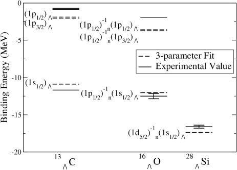
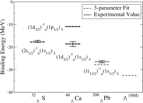
Figure 1: Results of the unweighted 3-parameter fit to a series of experimental data. The G2 parameter set of FST is used for both the nucleon and meson sectors [1]. The calculated binding energy of a single $\Lambda$ in infinite nuclear matter is also shown.

	M2	M3-1	M3-2	M4
$\chi^{2}_{10}(\mathrm{UW})\times 100$	0.105	0.0877
$\chi^{2}_{10}(\mathrm{W})\times 10$	0.598		0.515	0.485

Table 4: The $\chi^{2}$ values for both the unweighted (UW) and weighted (W) fits relative to the $\chi^{2}$ of the M1 set. Here $\chi^{2}$ is determined from Eq. (84) using 10 pieces of data.

In order to obtain a better fit to the data, we increase the level of truncation. Therefore, tensor couplings to both the vector and photon fields are included, which correspond to the terms in ${\cal L}_{\Lambda}^{\mathrm{(T)}}$. As a result, a third free parameter, $\mathrm{g_{T\Lambda}}$, is introduced. This fit is performed using seven pieces of experimental data: the six GS binding energies and the spin-orbit splitting given in Table 2. In this particular case, the weights in Eq. (84) are all taken to be equal. The resulting parameters are given in Table 3 as the M2 set and all satisfy the assumption of naturalness. Table 2 also outlines the numerical results of this 3-parameter fit. The outcome of this fit is shown graphically in Fig. 1. One can see that both the GS binding energies and the small spin-orbit splitting in the p-states are reproduced well. The calculated s-p shell excitation energies fail to duplicate the experimental values for the lightest $\Lambda$-hypernuclei; however, it is correctly given by the time one gets to ${}^{40}_{\Lambda}\mathrm{Ca}$. In Fig. 1, the value of $-32.4$ MeV is given as the calculated binding energy of a single $\Lambda$ in nuclear matter. This M2 parameter set will be used in the subsequent calculation of the $\mathrm{s}_{1/2}$-splittings.

A plot of the proton, neutron, and $\Lambda$ densities for the GS of ${}^{40}_{\Lambda}\mathrm{Ca}$ calculated using this M2 set is shown in Fig. 2. A graph of the Hartree spinors from the $\Lambda$ wave function, $\mathrm{G_{\Lambda}(r)}$ and $\mathrm{F_{\Lambda}(r)}$, for the GS of ${}^{40}_{\Lambda}\mathrm{Ca}$ using the M2 set is also given in Fig. 2. Notice that the magnitude of the lower spinor is very small; this indicates that the $\Lambda$ is essentially behaving as a nonrelativistic particle in the nuclear potential.

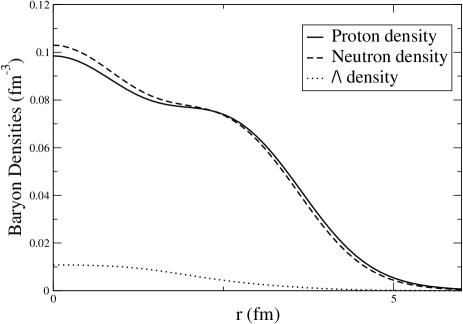
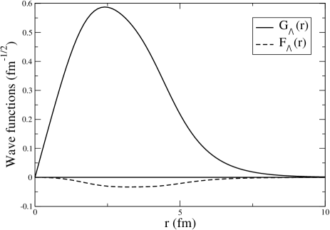
Figure 2: Top: plot of the proton, neutron, and lambda densities for the GS of ${}^{40}_{\Lambda}\mathrm{Ca}$. Bottom: radial wave functions of the $\Lambda$ in the $(1\mathrm{s}_{1/2})$ state for the GS of ${}^{40}_{\Lambda}\mathrm{Ca}$. Here the M2 parameter set was used.

Next, the two terms nonlinear in the scalar and vector field, shown in ${\cal L}_{\Lambda}^{\mathrm{(N)}}$, are retained. This brings the number of unconstrained parameters up to five. For this 5-parameter fit, ten pieces of experimental data are used; in addition to the data utilized in the 3-parameter fit, the three s-p shell $\Lambda$ excitation energies listed in Table 2 are also included. Two versions of the 5-parameter fit were conducted here: one unweighted and one weighted. In the former case, all of the weights are equal. For the latter, the weighting scheme is as follows: $\mathrm{W}_{\mathrm{X}}^{(i)}=1.0$ for GS binding energies; $\mathrm{W}_{\mathrm{X}}^{(i)}=10.0$ for s-p shell $\Lambda$ excitation energies; and $\mathrm{W}_{\mathrm{X}}^{(i)}=40.0$ for the spin-orbit splitting. The weights were selected using the formula $\mathrm{W}^{(i)}_{\mathrm{X}}=f_{i}(\mathrm{\Delta E_{exp}/E_{exp}})$ where $f_{i}$ is an arbitrary factor chosen to prevent any observable from dominating the fit [65]. However, not enough similar data was available to constrain the two new parameters individually. As a result, we initially restrict these parameters with the relation

$$\frac{\mu_{2}}{\mu_{1}}=\mathrm{\left(\frac{g_{S}\phi_{0}}{g_{V}V_{0}}\right)_{n.m.}^{2}}=1.624$$ (85)

where n.m. denotes the nuclear matter values [2]. The results of both 5-parameter fits are shown in Table 3; the M3-1 and M3-2 sets denote the unweighted and weighted schemes respectively. Again notice the parameters are all natural. However, the new parameters are not very well determined and fail to significantly improve the fit in either case, as can be seen from Table 4. Therefore, we leave the constraint of Eq. (85) intact.

Lastly, to include all possible terms in the $\Lambda$-lagrangian up to order $\nu=3$, all three terms in ${\cal L}_{\Lambda}^{\mathrm{(N)}}$ are retained. Again, not enough similar data was available to individually constrain the new parameters; therefore, we restrict these parameters with the relation

$$\mu_{1}=\mu_{3}=0.225\mu_{2}$$ (86)

and fix the remaining constants using the M2 set. These ratios were chosen because they tend to concentrate the effects of the new contributions in the surface of the nucleus, i.e. the additional contributions now vanish for uniform nuclear matter. This will have a greater effect on the s-p shell excitations than on the GSs. The weighting scheme described above was used. The resulting parameters are listed in Table 3 as the M4 set. Again, as seen in Table 4 the improvement in the overall fit is negligible. The M3-2 and M4 sets both improve the fit to the GSs but do worse with respect to the s-p shell excitations; the M3-1 set has the opposite effect. Also we mention that the parameter sets M3-1, M3-2, and M4 yield very similar density distributions to those acquired from the M2 set.

5.2 $\mathrm{s_{1/2}}$-splittings

In this section we discuss the calculation of the $\mathrm{s_{1/2}}$-splittings in $\Lambda$-hypernuclei and the results obtained from these calculations. Following the methodology established in section 4, one needs to evaluate $\delta\epsilon$ from Eq. (77) to determine the size of these doublets. It is possible to separate $\delta\epsilon$ into contributions from each portion of the effective interaction, or

$$\delta\epsilon=\delta\epsilon(\mathrm{s})+\delta\epsilon(\mathrm{vt})+\delta\epsilon(\mathrm{vs})$$ (87)

where s, vt, and vs represent the scalar, vector time, and vector spatial components respectively. As it turns out, the scalar and vector time components each cancel in the splitting, shown by

$$\mathrm{\delta\epsilon(s)=\delta\epsilon(vt)}=0$$ (88)

Therefore, the $\mathrm{s_{1/2}}$-splittings are entirely determined from the vector spatial term in the effective interaction, or

$$\delta\epsilon=\delta\epsilon(\mathrm{vs})$$ (89)

This is true for any system in which either the $\Lambda$ or the nucleon hole has $\mathrm{j=1/2}$. Note that this calculation tests a different sector of the underlying lagrangian than the mean field analysis and that, as there is no corresponding interpretation in the static limit $(\mathrm{M\rightarrow\infty})$, it is here an entirely relativistic effect. Now, to determine the splitting we only need to evaluate the matrix element in Eq. (LABEL:eqn:ph1) for the two appropriate J values. The integrals are solved using the Hartree spinors, $\mathrm{G}_{a}(\mathrm{r})$ and $\mathrm{F}_{a}(\mathrm{r})$, calculated in the single-particle analysis. Notice that the integrals in the vector spatial contribution mix the upper and lower components of the Hartree wave functions. Numerically, the integration is performed using Simpson’s method.

Nucleus	State	Levels	$|\delta\epsilon|$
${}^{12}_{\Lambda}\mathrm{B}$	$\mathrm{(1p_{3/2})_{p}^{-1}(1s_{1/2})_{\Lambda}}$	$2^{-}_{\mathrm{GS}}$, $1^{-}$	426
${}^{16}_{\Lambda}\mathrm{N}$	$\mathrm{(1p_{1/2})_{p}(1s_{1/2})_{\Lambda}}$	$1^{-}_{\mathrm{GS}}$, $0^{-}$	472
	$\mathrm{(1p_{3/2})_{p}^{-1}(1s_{1/2})_{\Lambda}}$	$2^{-}_{\mathrm{LL}}$, $1^{-}$	316
${}^{16}_{\Lambda}\mathrm{O}$	$\mathrm{(1p_{1/2})_{n}(1s_{1/2})_{\Lambda}}$	$1^{-}_{\mathrm{GS}}$, $0^{-}$	480
	$\mathrm{(1p_{1/2})_{n}(1p_{3/2})_{\Lambda}}$	$2^{+}_{\mathrm{LL}}$, $1^{+}$	125
	$\mathrm{(1p_{1/2})_{n}(1p_{1/2})_{\Lambda}}$	$1^{+}_{\mathrm{LL}}$, $0^{+}$	661
${}^{28}_{\Lambda}\mathrm{Si}$	$\mathrm{(1d_{5/2})_{n}^{-1}(1s_{1/2})_{\Lambda}}$	$3^{+}_{\mathrm{GS}}$, $2^{+}$	293
${}^{32}_{\Lambda}\mathrm{S}$	$\mathrm{(2s_{1/2})_{n}(1s_{1/2})_{\Lambda}}$	$1^{+}_{\mathrm{GS}}$, $0^{+}$	216
${}^{40}_{\Lambda}\mathrm{Ca}$	$\mathrm{(1d_{3/2})_{n}^{-1}(1s_{1/2})_{\Lambda}}$	$2^{+}_{\mathrm{GS}}$, $1^{+}$	308
	$\mathrm{(1d_{3/2})_{n}^{-1}(1p_{1/2})_{\Lambda}}$	$2^{-}_{\mathrm{LL}}$, $1^{-}$	393
${}^{208}_{\Lambda}\mathrm{Pb}$	$\mathrm{(1i_{13/2})_{n}^{-1}(1s_{1/2})_{\Lambda}}$	$7^{+}_{\mathrm{GS}}$, $6^{+}$	24

Table 5: $\mathrm{s_{1/2}}$-splittings, and some excited states, are shown with their respective configurations, level orderings, and doublet magnitudes. Here LL denotes lower level and $|\delta\epsilon|$ is in keV.

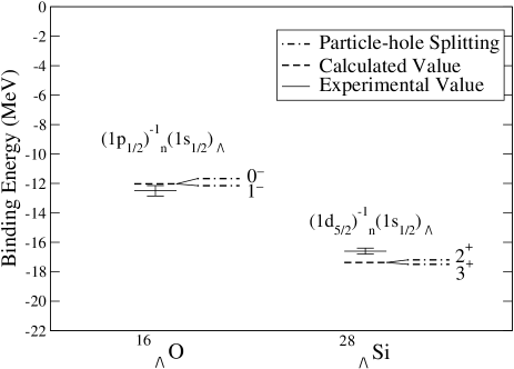
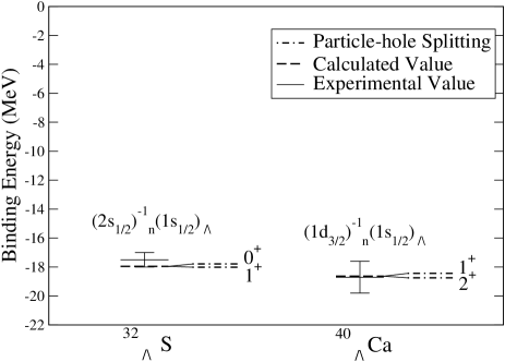
Figure 3: Graph of GS particle-hole splittings and their respective level orderings for ${}^{16}_{\Lambda}\mathrm{O}$ and ${}^{28}_{\Lambda}\mathrm{Si}$ on the top and ${}^{32}_{\Lambda}\mathrm{S}$ and ${}^{40}_{\Lambda}\mathrm{Ca}$ on the bottom. The single-particle calculations were conducted using the M2 parameter set and are plotted alongside the experimental values [47, 48, 49]. Notice that the splittings lie within the experimental error bars in all four cases.

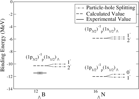
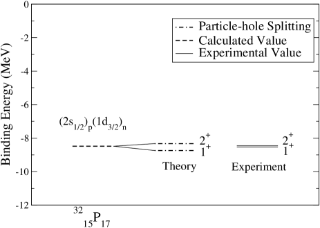
Figure 4: Top: graph of particle-hole splittings for ${}^{12}_{\Lambda}\mathrm{B}$ and ${}^{16}_{\Lambda}\mathrm{N}$ and their respective level orderings. In addition to the GSs, the first calculated excited state in ${}^{16}_{\Lambda}\mathrm{N}$ is also included. These calculations were conducted using the M2 parameter set. The experimental value for the GS of ${}^{12}_{\Lambda}\mathrm{B}$ is taken from [66]. Bottom: particle-hole splitting for the GS of ${}^{32}_{15}\mathrm{P}_{17}$. The level orderings and splittings are shown for both theory and experiment. Here the G2 parameter set of FST was used [1].

The results of this analysis are contained in Table 5. The splittings with a neutron hole listed in Table 5 all correspond to single-particle levels which were used in the fits of the preceding discussion, as shown in Fig. 1. The $\mathrm{s_{1/2}}$-splittings for ${}^{16}_{\Lambda}\mathrm{O}$, ${}^{28}_{\Lambda}\mathrm{Si}$, ${}^{32}_{\Lambda}\mathrm{S}$, and ${}^{40}_{\Lambda}\mathrm{Ca}$ are plotted in Fig. 3; notice that these four splittings are all within the experimental error bars and that the appropriate level orderings are shown. It should be mentioned that the three excited states with neutron holes shown in Table 5 will overlap with other states of the same J value. Therefore in these cases one must diagonalize the hamiltonian to determine the correct splitting and level ordering. The remaining doublets in Table 5, those with proton holes, are for predicted $\Lambda$ single-particle levels. These three are shown in Fig. 4; here, in addition to the GS splittings for both ${}^{12}_{\Lambda}\mathrm{B}$ and ${}^{16}_{\Lambda}\mathrm{N}$, the doublet for the first calculated excited state in ${}^{16}_{\Lambda}\mathrm{N}$ is also given. These splittings will be measured in an upcoming experiment using the reaction $\mathrm{(e,e^{\prime}K^{+})}$ with much greater resolution than the $\mathrm{(\pi^{+},K^{+})}$ reactions [58, 59]. As the effective interaction used here is isoscalar, there is no distinction in this approach between proton and neutron holes. This is apparent when comparing the GSs of ${}^{16}_{\Lambda}\mathrm{N}$ and ${}^{16}_{\Lambda}\mathrm{O}$; the slight difference in their splittings, which is only about 10 keV, arises from Coulomb effects. Also note that the splittings for configurations with the holes in the same shell are larger for the smaller j value. For example, the doublet for the GS of ${}^{12}_{\Lambda}\mathrm{B}$, in the $\mathrm{(1p_{3/2})_{p}^{-1}(1s_{1/2})_{\Lambda}}$ configuration, is smaller than that of the GS of ${}^{16}_{\Lambda}\mathrm{N}$, in the $\mathrm{(1p_{1/2})_{p}^{-1}(1s_{1/2})_{\Lambda}}$ state. The level orderings for each calculated doublet are also given in Table 5. Notice that for all of the cases considered here, the state with the higher J value is the GS or, in the case of excited states, the lower level.

Recent gamma-ray spectroscopy experiments [67] (and the experimental error bars on the GS binding energy of ${}^{12}_{\Lambda}\mathrm{B}$) suggest that these particle-hole splittings are in fact much smaller. In addition, the measured GS spins of ${}^{12}_{\Lambda}\mathrm{B}$ and ${}^{16}_{\Lambda}\mathrm{O}$ are 1 and 0 respectively [66, 68], whereas the values predicted here is 0 and 1 respectively. As the tensor coupling was important in the spin-orbit splittings, it may play an important role in the case of the $\mathrm{s}_{1/2}$-splittings. Higher order terms in the effective interaction, especially those involving the tensor coupling to the $\Lambda$, may be required to obtain a quantitative description of the small $\mathrm{s}_{1/2}$-doublet splitting and the correct level ordering. This is left for future work.

The present analysis was also extended to the case of ordinary nuclei. The necessary modifications to the theory were discussed in section 4. We apply this approach to the case of ${}^{32}_{15}\mathrm{P}_{17}$ in the $\mathrm{(2s_{1/2})_{p}(1d_{3/2})_{n}}$ state. As noted before, this calculation will require direct and exchange contributions from the scalar, vector, rho, and pion terms in the effective interaction. Fortunately, the statement of Eq. (88) holds here for the direct term and can be extended to include the direct rho time component as well. The result of our calculation is 413 keV; the observed value is 77 keV [60]. This is shown graphically in Fig. 4; notice that the correct magnitude and level ordering is obtained. However, it should be noted that this calculation is considerably more complicated than the $\Lambda$-N case.

In summary, we have successfully extended the hadronic effective field theory developed by FST to the region of the strangeness sector corresponding to single $\Lambda$-hypernuclei. This framework has the intrinsic strength of directly incorporating the following: special relativity, quantum mechanics, the underlying symmetry structure of QCD, and the nonlinear realization of spontaneously broken chiral symmetry. Furthermore, DFT provides a theoretical justification for this approach. This lagrangian can be used for predictive purposes once all the free parameters are determined. As a result, it was of interest to make a minimalist extension of this methodology in which a single, isoscalar $\Lambda$ is added to the theory. An appropriate $\Lambda$-lagrangian was constructed as an additional contribution to the full interacting lagrangian of FST. This system was solved using the Kohn-Sham analysis. Parameter fits were conducted at various levels of sophistication in the $\Lambda$-lagrangian while maintaining the full FST lagrangian with their G2 parameter set. The 3-parameter fit reproduces the GS binding energies and small spin-orbit splittings well, but fails to simulate fully the s-p shell excitations in the lightest hypernuclei, although by ${}^{40}_{\Lambda}\mathrm{Ca}$ the correct excitation energy is obtained. The inclusion of additional parameters does not significantly improve the quality of the fit.

Many of the GSs used in the fits were actually particle-hole states; as a result, it was of interest to calculate their splittings. A methodology for examining these splittings was developed using Dirac two-body matrix elements of an effective interaction. This effective interaction followed directly from the underlying lagrangian and to lowest order corresponded to simple scalar and vector exchange.${}^{\ref{foot:1}}$ Note that this lagrangian was designed to calculate other phenomena and there is nothing contained in it that guarantees the production of small particle-hole splittings. The primary conclusion from the present analysis is that all of the results obtained for the $\mathrm{s}_{1/2}$-doublet splittings used in the fitting procedure lie within the current experimental error bars. As a partial calibration, a calculation of the GS particle-hole splitting in ${}^{32}_{15}\mathrm{P}_{17}$, a much more complicated case, achieved the correct level ordering and doublet magnitude. Using this approach predictions were made for nuclei that will be measured in an upcoming $\mathrm{(e,e^{\prime}K^{+})}$ experiment at Jefferson Lab [58, 59].${}^{\ref{foot:1}}$

I would like to thank the following: Dr. J. D. Walecka for his support and advice; Dr. M. Huertas for the early use of a program he wrote to solve the Hartree equations [7] and for his help in its modification; and Dr. B. D. Serot for his careful reading of the manuscript and his helpful comments. This work was supported in part by DOE grant DE-FG02-97ER41023.

Appendix A

In this appendix, we discuss the selection of the terms in our $\Lambda$-lagrangian to order $\nu=3$. It is straightforward to see which terms are retained to order $\nu=2$, with the exception of the four fermion terms. Therefore, the following is a list of all remaining possible combinations of the fields to order $\nu=3$, consistent with this approach, and a short discussion of each.

• Four fermion terms in the nuclear case, such as $\mathrm{\bar{N}N\bar{N}N}$, are eliminated by substituting the meson equations of motion into the lagrangian. Under normal circumstances this is not feasible; however, this is allowed when the system is already in equilibrium. Here we want to extend the framework of FST to single $\Lambda$-hypernuclei with no additional mesons. In this case, either $\mathrm{\bar{N}N}\bar{\Lambda}\Lambda$ or $\bar{\Lambda}\Lambda\bar{\Lambda}\Lambda$ can be eliminated using this method, but not both simultaneously. Fortunately, the second term involves self-fields of the $\Lambda$ and consequently, can be discarded. This scheme also applies to terms with more than four fermion fields.

• The term $\bar{\Lambda}\sigma_{\mu\nu}\mathrm{V_{\mu\nu}}\Lambda$ is consistent with this framework.

• The terms $\bar{\Lambda}\Lambda\phi^{2}$ and $\bar{\Lambda}\Lambda\mathrm{V_{\mu}}^{2}$ are consistent with this framework. In the nucleon sector, terms of this variety were regrouped using meson field redefinitions. Here the terms have different constants than in the nucleon case; therefore, these terms cannot simply be regrouped, unless additional mesons are included.

• The term $\bar{\Lambda}\gamma_{\mu}\Lambda\phi\mathrm{V_{\mu}}$ is also retained. In the nuclear case, it was eliminated via the Dirac equation, but this is not possible here.

• Next, the following term is consistent with this methodology, but can be rewritten as

  $$\mathrm{\bar{\Lambda}\gamma_{\mu}\Lambda\frac{\partial\phi}{\partial x_{\mu}}}=\mathrm{\frac{\partial}{\partial x_{\mu}}\left(\bar{\Lambda}\gamma_{\mu}\Lambda\phi\right)}-\mathrm{\left[\frac{\partial}{\partial x_{\mu}}\left(\bar{\Lambda}\gamma_{\mu}\Lambda\right)\right]\phi}$$ (90)

  The second term is a total derivative, which does not change the action, and the third term is a four derivative of a conserved current, which is zero. Therefore this term can be neglected.

• Consider the following three terms: $\bar{\Lambda}\gamma_{\mu}\phi\mathrm{\frac{\partial}{\partial x_{\mu}}}\Lambda$, $\bar{\Lambda}\gamma_{\mu}\gamma_{\nu}\mathrm{V_{\mu}\frac{\partial}{\partial x_{\nu}}}\Lambda$, and $\bar{\Lambda}\gamma_{\mu}\gamma_{\nu}\mathrm{\frac{\partial}{\partial x_{\mu}}\frac{\partial}{\partial x_{\nu}}}\Lambda$. The Dirac equation for the $\Lambda$ can be substituted into each of these to convert them into a type of term already considered.

• Lastly, all of the contributions with $\mathrm{A_{\mu}}$ are absorbed into other terms in the same manner as like terms with $\mathrm{V_{\mu}}$. However, the terms $\bar{\Lambda}\gamma_{\mu}\Lambda\mathrm{A_{\mu}}$ and $\bar{\Lambda}\Lambda\mathrm{A_{\mu}^{2}}$ can be discarded as $\mathrm{Q=0}$ for the $\Lambda$. Therefore, the only remaining electromagnetic term is $\bar{\Lambda}\sigma_{\mu\nu}\mathrm{F_{\mu\nu}}\Lambda$.

Note that the parameters have yet to be determined. When the terms are regrouped, the free parameters can be redefined to suit our purposes.

References

- [1] R. J. Furnstahl, B. D. Serot, and H.-B. Tang, Nucl. Phys. A615, 441 (1997); (E) Nucl. Phys. A640, 505 (1998).
- [2] B. D. Serot and J. D. Walecka, Inter. J. of Mod. Phys. E6, 515 (1997).
- [3] A. Manohar and H. Georgi, Nucl. Phys. B234, 189 (1984).
- [4] H. Georgi, Phys. Lett. B298, 187 (1993).
- [5] J. D. Walecka, Theoretical Nuclear and Subnuclear Physics, Oxford University Press, Oxford 1995.
- [6] M. A. Huertas, Phys. Rev. C66, 024318 (2002); (E) Phys. Rev. C67, 019901 (2003).
- [7] M. A. Huertas, Ph.D. thesis, College of William and Mary (2003).
- [8] W. Kohn, Rev. Mod. Phys. 71, 1253 (1999).
- [9] B. D. Serot and J. D. Walecka, 150 Years of Quantum Many-Body Theory, World Scientific, Singapore 2001, p. 203.
- [10] R. Brockmann and W. Weise, Phys. Lett. 69B, 167 (1977).
- [11] J. Boguta and R. Bohrmann, Phys. Lett. 102B, 93 (1981).
- [12] J. V. Noble, Phys. Lett. B89, 325 (1980).
- [13] J. Mares and B. K. Jennings, Phys. Rev. C49, 2472 (1994);; Nucl. Phys. A585, 347c (1995).
- [14] J. Cohen and J. V. Noble, Phys. Rev. C46, 801 (1992).
- [15] J. Cohen and H. J. Weber, Phys. Rev. C44, 1181 (1991).
- [16] B. K. Jennings, Phys. Lett. B246, 325 (1990).
- [17] R. J. Lombard, S. Marcos, and J. Mares, Phys. Rev. C51, 1784 (1995).
- [18] N. K. Glendenning, D. Von-Eiff, M. Haft, H. Lenske, and M. K. Weigel, Phys. Rev. C48, 889 (1993).
- [19] L. L. Zhang, H. Q. Song, P. Wang, and R. K. Su, J. of Phys. G26, 1301 (2000).
- [20] P. Papazoglou, S. Schramm, J. Schaffner-Bielich, H. Stocker, and W. Greiner, Phys. Rev. C57, 2576 (1998).
- [21] P. Papazoglou, D. Zschiesche, S. Schramm, J. Schaffner-Bielich, H. Stocker, and W. Greiner, Phys. Rev. C59, 411 (1999).
- [22] Ch. Beckmann, P. Papazoglou, D. Zschiesche, S. Schramm, H. Stocker, and W. Greiner, Phys. Rev. C65, 024301 (2002).
- [23] H. Muller and J. Piekarewicz, J. of Phys. G27, 41 (2001).
- [24] H. Shen and H. Toki, Nucl. Phys. A707, 469 (2002).
- [25] K. Tsushima, K. Saito, and A. W. Thomas, Phys. Lett. B411, 9 (1997); (E) Phys. Lett. B421, 413 (1998).
- [26] C. M. Keil, F. Hoffmann, and H. Lenske, Phys. Rev. C61, 064309 (2000).
- [27] D. J.Millener, C. B. Dover, and A. Gal, Phys. Rev. C38, 2700 (1988).
- [28] Y. Yamamoto, H. Bando, and J. Zofka, Prog. Theor. Phys. 80, 757 (1988).
- [29] E. D. Cooper, B. K. Jennings, and J. Mares, Nucl. Phys. A580, 419 (1994); Nucl. Phys. A585, 157c (1995).
- [30] O. Hashimoto, Hyper. Int. 103, 245 (1996).
- [31] Th. A. Rijken, Nucl. Phys. A639, 29c (1998).
- [32] Th. A. Rijken, V. G. J. Stoks, and Y. Yamamoto, Phys. Rev. C59, 21 (1999).
- [33] D. Halderson, Phys. Rev. C60, 064001 (1999).
- [34] A. Reuber, K. Holinde, and J. Speth, Nucl. Phys. A570, 543 (1994).
- [35] J. Hao and T. T. S. Kuo, Phys. Rep. 264, 233 (1996).
- [36] I. Vidana, A. Polls, A. Ramos, and M. Hjorth-Jensen, Nucl. Phys. A644, 201 (1998).
- [37] Y. Yamamoto, S. Nishizaki, and T. Takatsuka, Prog. Theor. Phys. 103, 981 (2000).
- [38] J. Cugnon, A. Lejeune, and H. J. Schulze, Phys. Rev. C62, 064308 (2000).
- [39] I. Vidana, A. Polls, A. Ramos, and H. J. Schulze, Phys. Rev. C64, 044301 (2001).
- [40] S. Fujii, R. Okamoto, and K. Suzuki, Nucl. Phys. A651, 411 (1999).
- [41] M. Kohno, Y. Fujiwara, T. Fujita, C. Nakamoto, and Y. Suzuki, Nucl. Phys. A670, 319c (2000); Nucl. Phys. A674, 229 (2000b).
- [42] D. E. Lanskoy and Y. Yamamoto, Phys. Rev. C55, 2330 (1997).
- [43] Q. N. Usmani and A. R. Bodmer, Phys. Rev. C60, 055215 (1999).
- [44] F. Arias de Saavedra, G. Co, and A. Fabrocini, Phys. Rev. C63, 064308 (2001).
- [45] M. Oka, Nucl. Phys. A629, 379c (1998).
- [46] C. Dover, H. Feshbach, and A. Gal, Phys. Rev. C51, 541 (1995).
- [47] P. H. Pile, et al., Phys. Rev. Lett. 66, 2585 (1991).
- [48] R. Bertini, et al., Phys. Lett. 83B, 306 (1979).
- [49] T. Hasagawa, et al., Phys. Rev. C53, 1210 (1996).
- [50] H. Kohri, et al., Phys. Rev. C65, 034607 (2002).
- [51] T. Takahashi, et al., Nucl. Phys. A670, 265c (2000).
- [52] T. Cantwell, et al., Nucl. Phys. A236, 445 (1974).
- [53] A. Fetter and J. D. Walecka, Quantum Theory of Many-particle Systems McGraw-Hill, 1971.
- [54] R. J. Furnstahl, Phys. Lett. 152B, 313 (1985).
- [55] V. G. J. Stoks and Th. A. Rijken, Phys. Rev. C59, 3009 (1999).
- [56] P. M. M. Maessen, Th. A. Rijken, and J. J. de Swart, Phys. Rev. C40, 2226 (1989).
- [57] A. Edmonds, Angular Momentum in Quantum Mechanics Princeton University Press, Princeton 1957.
- [58] F. Garibaldi, et al., E-94-107 proposal: High resolution hypernuclear 1p shell spectroscopy (1994).
- [59] G. M. Urciuoli, et al., Nucl. Phys. A691, 43c (2001).
- [60] J. D. Walecka, Annals of Phys. 63, 219 (1971).
- [61] A. De-Shalit and J. D. Walecka, Nucl. Phys. 22, 184 (1961).
- [62] H. Matsunobu and H. Takebe, Prog. of Theor. Phys. 14, 589 (1955).
- [63] M. Rotenberg, R. Bivins, N. Metropolis, and J. Wooten, The 3-j and 6-j Symbols The Technology Press, Cambridge 1959.
- [64] J. McIntire, Phys. Rev. C66, 064319 (2002).
- [65] B. A. Nikolaus, T. Hoch, and D. G. Madland, Phys. Rev. C46, 1757 (1992).
- [66] M. Juric, et al., Nucl. Phys. B52, 1 (1973).
- [67] H. Tamura, et al., Mod. Phys. Lett. 18, 85 (2003).
- [68] D. J. Millener, nucl-th/0402091.