Quantitative Relativistic Effects in the Three-Nucleon Problem

Abstract

The quantitative impact of the requirement of relativistic invariance in the three-nucleon problem is examined within the framework of Poincaré invariant quantum mechanics. In the case of the bound state, and for a wide variety of model implementations and reasonable interactions, most of the quantitative effects come from kinematic factors that can easily be incorporated within a non-relativistic momentum-space three-body code.

I Introduction

Advances in computational algorithms as well as hardware speed have enabled a new era of precision calculations in the few-nucleon sector. It is now possible to compute binding properties, and in some cases other properties, of nuclei up through A=10, starting with the Schrödinger equation plus phenomenological two- and three-body interactions, to a precision that allows for a meaningful comparison between theory and experiment.

Computations are now precise enough that the quantitative role of special relativity becomes relevant. In principle, Poincaré invariance is an exact symmetry that should be satisfied by all numerical calculations, thereby permitting comparisons between theory and experiment to rest entirely upon the nuclear dynamics. In practice,

1. Consistent relativistic computation is much more numerically intensive, thus motivating non-relativistic calculations in practice.

2. Most estimates of relativistic effects have been quantitatively small enough that the non-relativistic calculations have satisfactory precision.

An additional complication is that a non-relativistic model does not imply a unique relativistic extension. Relativistic invariance requires the invariance of probabilities in different inertial coordinate systems; this symmetry can be satisfied in a variety of frameworks and models that share the same non-relativistic limit. Since information is lost in taking the non-relativistic limit, there is no unique way to get it back.

At the two-body level, calculations in a single inertial coordinate system are not constrained by Poincaré invariance; it only ensures that the results in all other inertial coordinate systems are equivalent. This affects how the two-body dynamics is embedded in the three-body problem. In addition, there is a unitary group of three-body scattering equivalences that preserves Poincaré invariance and leaves the two and three-body scattering and bound state observables unchanged, at the expense making off-shell modifications and modifications to the two and three-body interactions. This freedom is not constrained by experiment. This means that the contributions of relativistic effects, off-shell effects, and three-body interactions cannot be uniquely separated in the three-body problem.

Therefore, there is no single, unique “relativistic effect” in few-nucleon calculations. However, we find that, for a variety of dynamical input and some variation in model assumptions, there is a consistent pattern in the quantitative aspects of relativity in the calculations.

There are two primary approaches for modeling relativistic few-body problems in quantum mechanics. We consider here a class of Poincaré invariant quantum models Wigner (1939) of few-particle systems. In these models Poincaré invariance is an exact symmetry that is realized by a unitary representation of the Poincaré group on the few-particle Hilbert space. A number of equivalent representations of Poincaré invariant few-body models are given in Bakamjian and Thomas (1953); Keister and Polyzou (1991). Poincaré invariant quantum mechanics has as its starting point a Hilbert space with a fixed number of particles (nucleons) and a set of 2-, 3-,… body interactions. These features it shares with its non-relativistic counterpart based upon the Schrödinger equation. It differs from the latter in the relationship between interactions in different inertial reference frames. At the level of two-body phenomenology, one can make connections to parameters fitted to data on the basis of the Schrödinger equation. If this is done in one inertial coordinate system, the Poincaré invariance can be used to generate interactions in any other inertial frame. There are several ways to do this, as will be discussed below.

Glöckle, Kamada, and collaborators Kamada and Glöckle (1998); Kamada et al. (2002); Kamada and Glöckle (2004) have studied aspects of Poincaré invariant quantum mechanics in two- and three-body problems. They have introduced a mapping between the interactions in the relativistic two-body mass operator and the interactions in the non-relativistic center-of-momentum two-body Hamiltonian, and have solved the three-body problem for specific interactions Witala et al. (2005). Different methods for utilizing realistic nucleon-nucleon interactions in relativistic calculations were given by Coester, Pieper and Serduke Coester et al. (1975) and by Glöckle, Lee, and Coester Glöckle et al. (1986). Our goal here is to identify the dominant sources of relativistic effects for a variety of two-body mappings and interactions.

The second approach to the relativistic few-body problem uses quasipotential equations. These are relations between covariant amplitudes in local field theory. When some of the amplitudes are treated as input, these relations become equations for the remaining amplitudes. Matrix elements of few-body observables in eigenstates of the four momentum can be calculated from the solution of the quasipotential equations using Mandelstam’s method Mandelstam (1955); Huang and Weldon (1975). For systems of strongly interacting particles, the input to these equations is not known and must be modeled, as in Poincaré invariant quantum mechanics. While calculations of the same observables can be computed in both approaches, there exist no unique relation between quasipotential equations and Poincaré invariant quantum mechanics. Nevertheless, quasipotential models have played a historically important and valuable role in motivating the structure of model nucleon-nucleon interactions. The nature of the relativistic effects depends upon the specific assumptions used to extract quantum mechanical interactions from the quasipotential equations. Stadler and Gross Stadler and Gross (1997) have studied solutions to the three-nucleon bound state problem in the context of the spectator approximation to a meson-nucleon field theory. Sammarruca and Machleidt Sammarruca and Machleidt (1998) have studied specific kinematic factors that arise in extracting quantum mechanical interactions from quasipotential equations in an effort to identify the dominant sources of relativistic effects.

In this paper, we attempt to identify the important quantitative relativistic effects within the framework of Poincaré invariant quantum mechanics. The goal in this paper is not to provide complete solutions to a set of three-body problems, but rather to understand where the major relativistic effects occur. In fact, the most important effects are embedded in multiplicative kinematic factors, which makes it relatively easy to incorporate them into a Schrödinger-based momentum-space three-body code.

II The Two-Body Problem

One-nucleon momentum/spin eigenstates satisfy the normalization condition:

$$\langle{\bf p}^{\prime},\mu^{\prime}|{\bf p},\mu\rangle=\delta({\bf p}^{\prime}-{\bf p})\delta_{\mu^{\prime}\mu}.$$ (1)

These states transform as mass $m$ spin $1/2$ irreducible representations of the Poincaré group Keister and Polyzou (1991). For the two-body problem it is useful to use a basis that transforms irreducibly with respect to the tensor product of two one-body representations. These Poincaré irreducible eigenstates have the structure

$$|{\bf P},j,\mu,k;l,s\rangle$$ (2)

where ${\bf P}$ is the total linear momentum, $j$ is the canonical spin, $\mu$ is the $z$-component of the canonical spin, and $k$ is related to the invariant invariant mass of the non-interacting two-body system by

$$M^{(0)}=2\sqrt{m^{2}+k^{2}}.$$ (3)

The quantum numbers $l$ and $s$ are degeneracy quantum numbers that determine the multiplicity of each representation with the same $M^{(0)}$ and $j$; $l$ and $s$ have the same spectrum as the non-relativistic total spin and orbital angular momentum quantum numbers. The overlap coefficients with the tensor product of single particle states are Poincaré Clebsch-Gordan coefficients which can be found in (Joos (1962)Coester (1965)Keister and Polyzou (1991)Moussa and Stora (1964)).

The two-body mass operator is defined by adding interactions to the non-interacting mass operator:

$$M=M^{(0)}+v.$$ (4)

In Poincaré invariant quantum mechanics the delta functions that multiply interactions are important. The two-body interaction acting on the two-body Hilbert space is denoted by $v$; $\bar{v}$ denotes the internal two-body interaction related to $v$ by

$$\langle{\bf P}^{\prime},j^{\prime},\mu^{\prime},k^{\prime},l^{\prime},s^{\prime}|v|{\bf P},j,\mu,k,l,s\rangle=$$

$$\delta({\bf P}^{\prime}-{\bf P})\delta_{j^{\prime}j}\delta_{\mu^{\prime}\mu}\langle k^{\prime},l^{\prime},s^{\prime}|\bar{v}^{j}|k,l,s\rangle.$$ (5)

With this choice of $v$ it is possible to find simultaneous eigenstates of $M$, ${\bf P}$, $j^{(0)}$, and ${\bf j}^{(0)}\cdot\hat{\bf z}$. These states transform like mass $M$, spin ${\bf j}^{(0)}$ irreducible representations of the Poincaré group. Since these eigenstates are complete they define the interacting two-body dynamics.

Two-particle scattering is described by the transition operator

$${t}(e)={v}+{v}{1\over{e+i0-M}}{v}$$ (6)

which satisfies the relativistic Lippmann-Schwinger equation:

$${t}(e)={v}+{v}{1\over{e+i0-M^{(0)}}}{t}(e).$$ (7)

This transition operator has the same relation to the differential cross section as the corresponding non-relativistic expression, except that the single particle masses, $m$, appearing in the incident current and phase space factors are replaced by the corresponding single particle energies, $\omega=\sqrt{k^{2}+m^{2}}$. A proof based on time-dependent scattering theory is given in Keister and Polyzou (1991).

The reduced two-body transition operator $\bar{t}(e)$ is related to $t(e)$ by

$$\langle{\bf P}^{\prime},j^{\prime},\mu^{\prime},k^{\prime},l^{\prime}s^{\prime}|t(e)|{\bf P},j,\mu,k,l,s\rangle=$$

$$\delta({\bf P}^{\prime}-{\bf P})\delta_{j^{\prime}j}\delta_{\mu^{\prime}\mu}\langle k^{\prime},l^{\prime},s^{\prime}|\bar{t}^{j}(e)|k,l,s\rangle.$$ (8)

III Connections to Two-Body Phenomenology

All realistic descriptions of the quantum mechanical two-nucleon system utilize adjustable parameters in the interactions to fit published nucleon-nucleon phase-shift data and the deuteron binding energy. For Poincaré invariant quantum mechanical models, these parameters involve interaction strengths and ranges; for quasipotential models, the parameters may include meson-nucleon coupling strengths and form factors. Since there is an extensive investment of effort in fitting nucleon-nucleon data to solutions to the Schrödinger equation, it is advantageous to directly use existing high-quality interactions to construct equivalent relativistic interactions.

The relationship between relativistic and non-relativistic models fit to the same data is more complicated than the relation obtained by taking the non-relativistic limit of the relativistic model. Understanding the nature of the fitting process is the first element needed to understand the nature of relativistic corrections. The scattering cross section is a relativistic invariant Møller (1945); however, the angular distributions and spins have a frame dependence with known kinematic transformation properties. Kinematic Lorentz transformations are used to correctly transform measured laboratory differential scattering cross sections to the center of momentum frame. The properly transformed data are used to fit interactions that reproduce this data by solving the non-relativistic Schrödinger equation.

The scattering operator and consequently the phase shifts for a given angular momentum are Poincaré invariant. The phase shifts can be tabulated as functions of the invariant center of momentum momentum or energy, $\delta_{j}(k)$ or $\delta^{\prime}_{j}(e)$. These functions are equal when the center of momentum energy $e$ and invariant momentum $k$ are related by the correct relativistic relation. For equal mass particles this relation is $e=2\sqrt{k^{2}+m^{2}}$ which implies

$$\delta_{j}(k)=\delta^{\prime}_{j}(2\sqrt{m^{2}+k^{2}})\qquad\delta^{\prime}_{j}(e)=\delta_{j}\left(\sqrt{{e^{2}\over 4}-m^{2}}\right).$$ (9)

In the fitting procedure these phase shifts are identified with phase shifts obtained by solving the Schrödinger equation. This can be done in one of two inequivalent ways Allen et al. (2000). The first is by identifying $\delta_{j}(k)$ with the corresponding $k$-dependent Schrödinger phase shift and the second is by identifying $\delta_{j}^{\prime}(e)$ with the corresponding $e$-dependent Schrödinger phase shift. These are inequivalent because non-relativistically $e$ and $k$ are related by $e=k^{2}/m+2m$.

If these procedures are used there are no relativistic corrections in the center of momentum frame when compared to a relativistic model fit to the same data. The Schrödinger equation produces the exact Poincaré invariant phase shifts either as functions of the center of momentum energy or momentum (but not both).

The problem that can arise is if the phase shifts are fit to transformed cross section data as functions of $k$ and the potential is constructed by matching the phase shifts obtained from the Schrödinger equation as functions of $e$, then the phase shift or cross section predicted at energy $e=k^{2}/m+2m$ will be the same as the “measured” phase shift a shifted energy $e^{\prime}=2\sqrt{m^{2}+k^{2}}$. Similarly, if the phase shifts are fit to transformed cross section data as functions of $e$ and the potential is constructed by matching the phase shifts obtained from the Schrödinger equation as functions of $k$ then the phase shift or cross section predicted at momentum $k=\sqrt{em-2m^{2}}$ will be the same as the measured phase shift a shifted momentum $k^{\prime}=\sqrt{e^{2}/4-m^{2}}$.

This inconsistency increases with momentum. At relativistic energies the inconsistencies are of the same scale as typical relativistic corrections. This is illustrated in Figure 1, which compares the non-relativistic and relativistic energies $e_{nr}(k)$ to $e_{r}(k)$ for a nucleon with momenta $k$ up to 1 GeV. These curves show the scale of the energy mismatch as a function of $k$; it is a 7% effect at 1 GeV. Figure 2 illustrates the same effect with the total cross section. The curves in Figure 2 compare the total cross sections in the Born approximation for the Malfliet-Tjon V potential Malfliet and Tjon (1969). The curve in Figure 2 is the ratio $\sigma(k)/\sigma(k\sqrt{1+k^{2}/4m^{2}})$ for $k$ up to 1 GeV/$c$. In this example figure shows that an inconsistent treatment of the phase equivalence, while small at low momenta, leads to a 15% percent error in the total cross section at 1 GeV/$c$.

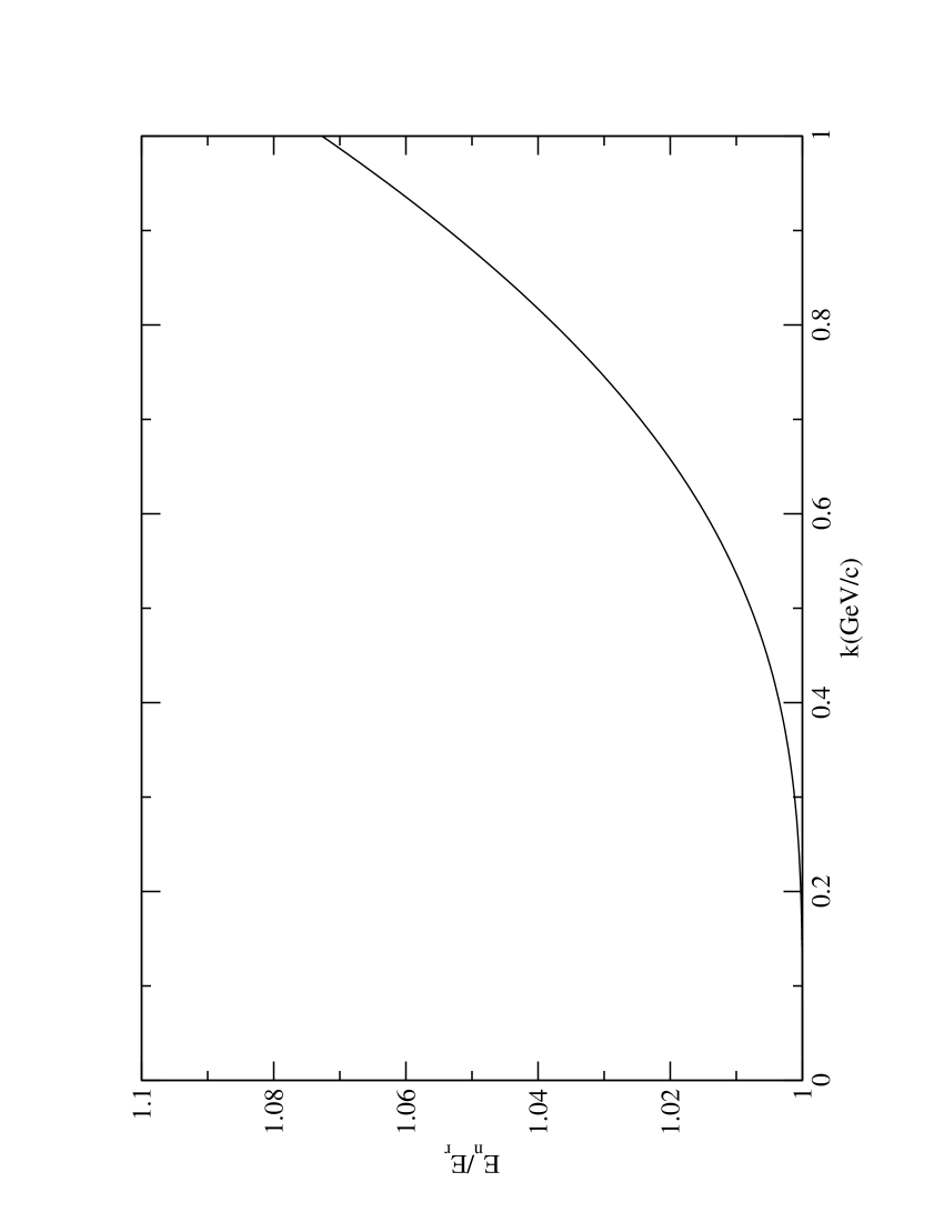
Figure 1: Relativistic vs Non-relativistic CM energy as a function of $k$.

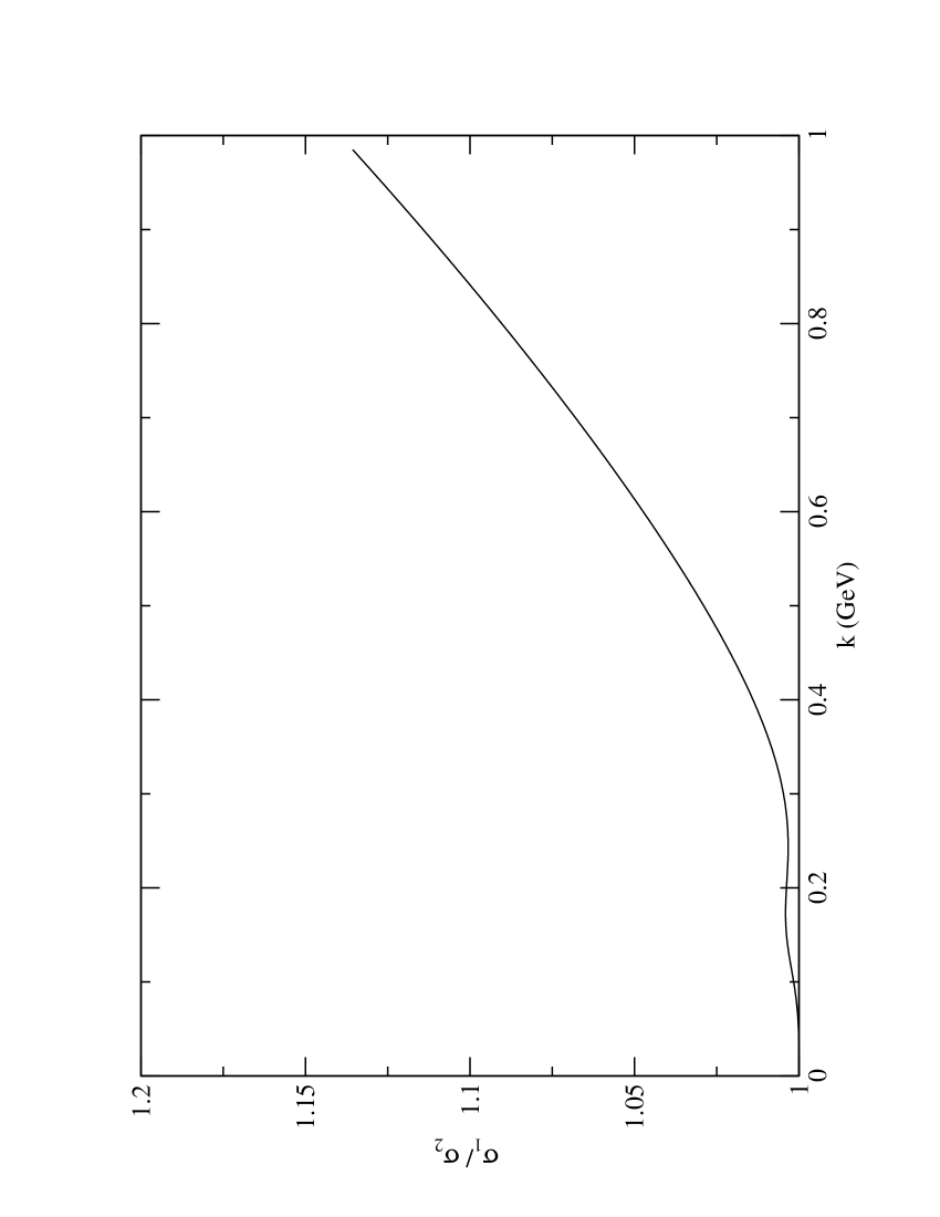
Figure 2: Differences in invariant cross section identified as functions of relative momentum to relative energy.

Thus, the first question that needs to be considered is how the non-relativistic interaction was constructed. For Argonne $V18$, which is a typical example of a realistic nucleon-nucleon interaction, the phase shifts are determined as functions of laboratory beam energy Wiringa, Stoks and Schiavilla (1995) which is converted to center-of-momentum momentum using

$$-p_{b}\cdot p_{t}=e_{Lab}m=(k^{2}+m^{2})+k^{2}.$$ (10)

Thus, for the $AV18$ interaction, the solution of the Schrödinger equation reproduces the invariant phase shifts $\delta_{j}(k)$ as functions of the invariant momentum.

The methods discussed in this paper make use of the phase equivalence between the interactions in the relativistic and non-relativistic Schrödinger equations. We consider three ways of utilizing two-body phenomenology based upon the fitted interactions in Schrödinger equation in Poincaré invariant quantum mechanics. These methods relate the half-shell relativistic two-body transition matrix elements to the half-shell non-relativistic transition matrix elements under different sets of assumptions about the phase shift fitting.

III.1 Coester-Pieper-Serduke (CPS)

This method was formulated to study relativistic effects in nuclear matter. It uses a nucleon-nucleon interaction, such as $AV18$, fit to $\delta_{j}(k)$ to construct a scattering equivalent relativistic interaction.

CPS Coester et al. (1975) add an interaction to the square of the non-interacting mass operator to get a Schrödinger-like equation:

$$M^{2}=M^{(0)2}+{u}=4mh\qquad h:={k^{2}\over m}+{{u}\over 4m}+m.$$ (11)

The operator ${u}/4m={v}_{nr}$ is identified with the interaction that appears in the non-relativistic Schrödinger Hamiltonian, $h$.

The relationship between ${u}$ in Eq. (11) and the relativistic interaction ${v}$ in Eq. (5) is

$${u}={v}^{2}+\{M^{(0)},{v}\}.$$ (12)

It would be tedious to evaluate ${v}$ directly; however, it is never needed because $M$, $M^{2}$ and $h=k^{2}/m+{v}_{nr}$, all have the same eigenstates.

If ${\hat{t}}(e)$ is generated by the “Lippmann-Schwinger” equation

$${\hat{t}}(e)={u}+{u}{1\over e^{2}-M^{(0)2}+i0^{+}}\hat{t}(e),$$ (13)

and $|\psi_{k}^{+}\rangle$ is a scattering eigenstate with momentum $k$ and $|\psi_{k}\rangle$ is the corresponding plane wave state, then the following half-shell relations follow:

$${t}(e(k))|\psi_{k}\rangle={v}|\psi_{k}^{+}\rangle=(M-M_{0})|\psi_{k}^{+}\rangle=$$

$${1\over e(k)+M_{0}}(M^{2}-M_{0}^{2})|\psi_{k}^{+}\rangle=$$

$${1\over e(k)+M_{0}}{u}|\psi_{k}^{+}\rangle={1\over e(k)+M_{0}}\hat{t}(e(k))|\psi_{k}\rangle=$$

$${4m\over e(k)+M_{0}}{v}_{nr}|\psi_{k}^{+}\rangle={4m\over e(k)+M_{0}}{t}_{nr}(e_{nr}(k))|\psi_{k}\rangle.$$ (14)

Taking matrix elements in the irreducible plane wave states $|k,j,l,s\rangle$ gives the relation

$$\langle k^{\prime},l^{\prime},s^{\prime}|\bar{t}^{j}(e(k))|k,l,s\rangle=$$

$$[e(k)+e(k^{\prime}))]^{-1}\langle k^{\prime},l^{\prime},s^{\prime}|{\hat{t}}^{j}(e(k))|k,l,s\rangle=$$

$${4m\over e(k)+e(k^{\prime})}\langle k^{\prime},l^{\prime},s^{\prime}|{\bar{t}}_{nr}^{j}(k^{2}/m)|k,l,s\rangle$$ (15)

where $e(k)=2\omega(k)=2\sqrt{k^{2}+m^{2}}$, $e_{nr}(k)=k^{2}/m$, and $\bar{t}^{j}$ is the reduced non-relativistic two-body transition operator.

This gives the desired relation between the relativistic and non-relativistic half off-shell transition matrix elements. This formula will be used to construct the kernel of the three-body equations.

It has been shown that for the CPS method the relativistic and non-relativistic cross sections are identical functions of the invariant momentum $k$ Keister and Polyzou (1991), and the relativistic and non-relativistic bound states have the same bound-state wave numbers. This phase equivalence is exact.

III.2 Glöckle-Lee-Coester (GLC)

Glöckle,Lee and Coester introduced an approximate variation of the CPS method that did not require introducing the interaction ${u}$. This approximation was used in the first calculation of a three-body binding energy based on Poincaré invariant quantum mechanics Glöckle et al. (1986).

Like the CPS method, the GLC method uses a nucleon-nucleon interaction, such as $AV18$ Wiringa, Stoks and Schiavilla (1995), fit to $\delta_{j}(k)$ to construct a scattering equivalent relativistic interaction. In this case the scattering equivalence is only approximate.

GLC Glöckle et al. (1986) define a new interaction:

$$\langle k^{\prime},l^{\prime},s^{\prime}|{\bar{v}}_{nr}^{j}|k,l,s\rangle=\sqrt{\omega^{\prime}\over m}\langle k^{\prime},l^{\prime},s^{\prime}|\bar{v}^{j}|k,l,s\rangle\sqrt{\omega\over m},$$ (16)

with the corresponding $t$ matrix elements:

$$\langle k^{\prime},l^{\prime},s^{\prime}|{\bar{t}}^{j}_{nr}(k^{2}/m)|k,l,s\rangle:=$$

$$\sqrt{\omega^{\prime}\over m}\langle k^{\prime},l^{\prime},s^{\prime}|\bar{t}^{j}(e(k))|k,l,s\rangle\sqrt{\omega\over m}.$$ (17)

Equation (17) replaces (15) in the CPS method. With the above definitions if $\bar{t}$ satisfies the relativistic Lippmann-Schwinger equation, it does not follow that $\bar{t}_{nr}$ will satisfy the non-relativistic Lippmann Schwinger equation, however is straightforward to derive

$$\langle k^{\prime},l^{\prime},s^{\prime}|{\bar{t}}_{nr}^{j}(k^{2}/m)|k,l,s\rangle=\langle k^{\prime},l^{\prime},s^{\prime}|{\bar{v}}_{nr}^{j}|k,l,s\rangle+$$

$$\sum_{l^{\prime\prime}s^{\prime\prime}}\int k^{\prime\prime 2}dk^{\prime\prime}\,{\langle k^{\prime},l^{\prime},s^{\prime}|{\bar{v}}^{j}_{nr}|k^{\prime\prime},l^{\prime\prime},s^{\prime\prime}\rangle\over k^{2}/m-k^{\prime\prime}{}^{2}/m+i0}\times$$

$$\langle k^{\prime\prime},l^{\prime\prime},s^{\prime\prime}|{\bar{t}}^{j}_{nr}(k^{2}/m)|k,l,s\rangle\left[1+{\omega-\omega^{\prime\prime}\over 2\omega^{\prime\prime}}\right].$$ (18)

The CPS approximation is equivalent to neglecting the term, ${\omega-\omega^{\prime\prime}\over 2\omega^{\prime\prime}}$, which is zero on shell. Neglecting this term gives the non-relativistic Lippmann-Schwinger equation. CPS approximate the solution, $\bar{t}^{j}_{nr}$, of (18) by the non-relativistic transition operator.

It can be shown that this method does not lead to an exact phase equivalence, it is possible to construct systematic corrections that converge to the $CPS$ result. In the original CPS calculation this approximation was found to be accurate. It was improved using a slight adjustment of the interaction parameters.

III.3 Glöckle-Kamada (GK)

The GK approach is designed to produce a relativistic dynamical model that is phase equivalent to a corresponding non-relativistic model where the phases shifts are fit as functions of center of momentum energy, $\delta^{\prime}(E)$.

The GK Kamada and Glöckle (1998) approach uses a unitary rescaling of the momentum variables to change the non-relativistic kinetic energy into the relativistic kinetic energy.

For each value of the momentum $k$, GK define the momentum $q$ by identifying the relativistic and non-relativistic energies

$$2m+{q^{2}\over m}=2\sqrt{m^{2}+k^{2}}.$$ (19)

This can solved for be either for $k(q)$ or $q(k)$. Defining $h(q)$ as

$$h^{2}(q):={q^{2}\over k^{2}}{dq\over dk}$$ (20)

Glöckle and Kamada identify a “relativistic” interaction:

$$\langle k^{\prime},l^{\prime},s^{\prime}|{\bar{v}}^{j}|k,l,s\rangle:=$$

$$h(k^{\prime})\langle q(k^{\prime}),l^{\prime},s^{\prime}|\bar{v}^{j}_{nr}|q(k),l,s\rangle h(k)$$ (21)

and $t$ matrix:

$$\langle k^{\prime},l^{\prime},s^{\prime}|{\bar{t}}^{j}(e(k))|k,l,s\rangle:=$$

$$h(k^{\prime})\langle q(k^{\prime}),l^{\prime},s^{\prime}|\bar{t}_{nr}^{j}(e_{nr}(q(k))|q(k),l,s\rangle h(k).$$ (22)

Then $\bar{t}^{j}$ and ${\bar{t}}^{j}_{nr}$ satisfy the relativistic and non-relativistic Lippmann-Schwinger equations, as functions of $k$ or $q$, respectively.

With this method (22) replaces (17) or (15).

In Kamada and Glöckle (1998) Kamada and Glöckle show that with the KG method the relativistic and non-relativistic phase shifts are identified as functions of the invariant energy $E$, and the relativistic and non-relativistic bound states have identical binding energy.

IV The Three-Body Problem

To construct kinematic variables for the three-body system, let $M^{(0)}$ denote the invariant mass of the non-interacting three-body system and $M^{(0)}_{ij}$ be the invariant mass for the non-interacting two-body sub-system consisting of particles $i$ and $j$.

Plane-wave basis states are tensor products of one-body Poincaré irreducible representation space basis vectors

$$|{\bf p}_{1},\nu_{1},{\bf p}_{2},\nu_{2},{\bf p}_{3},\nu_{3}\rangle.$$ (23)

As in the non-relativistic case it is useful to define the total momentum

$${\bf P}:=\sum_{i=1}^{3}{\bf p}_{i}$$ (24)

and relativistic Jacobi momenta, which are the the three-vector components of

$$K_{ij}^{\mu}:=L^{-1}({{\bf P}\over M^{(0)}})^{\mu}{}_{\nu}p_{k}^{\nu}$$ (25)

$$k_{ij}^{\mu}:=L^{-1}({{\bf p}_{i}+{\bf p}_{j}\over M^{(0)}_{ij}})^{\mu}{}_{\nu}p_{i}^{\nu}$$ (26)

where $L(\cdot)$ denotes a rotationless (canonical) Lorentz boost. These choices are appropriate for an “instant-form” representation. We use this representation for the purpose of illustration. Other choices give similar formulas.

The non-relativistic Jacobi moment are obtained if the Lorentz boosts $L$ are replaced by the corresponding Galilean boosts. Both the relativistic and corresponding Jacobi momentum operators have identical spectra.

For the three-body problem it is useful to successively pairwise couple the one-body Poincaré irreducible representations to obtain three-body Poincaré irreducible basis vectors. This is done using pairs of Poincaré Clebsch-Gordan coefficients. There are three bases that differ in the order of the pairwise coupling. We use the following shorthand notation for the basis that couples the irreducible representation associated with the pair $(kl)$ to the representation associated with the “spectator” particle, $m$:

$$|{\bf P},j,\mu,(kl)(m)\rangle:=|{\bf P},j,\mu;L_{kl},S_{kl},K_{kl},j_{kl},l_{kl},s_{kl},k_{kl}\rangle.$$ (27)

Here $K_{kl}$ and $k_{kl}$ are magnitudes of the relativistic Jacobi momenta. They are related to the invariant masses of the two- and three-body irreducible representation by

$$M^{(0)}_{kl}=2\sqrt{{k}_{kl}^{2}+m^{2}}$$ (28)

and

$$M^{(0)}=\sqrt{M^{(0)}_{kl}{}^{2}+{K}_{kl}^{2}}+\sqrt{m^{2}+{K}_{kl}^{2}}.$$ (29)

The two-body interaction $V_{kl}$ and reduced two-body interaction $\bar{V}_{kl}$ are defined in this basis by

$$\langle{\bf P},j,\mu,(kl)(m)|V_{kl}|{\bf P}^{\prime},j^{\prime},\mu^{\prime},(kl)(m)^{\prime}\rangle=$$

$$\delta({\bf P}-{\bf P}\,^{\prime})\delta_{jj^{\prime}}\delta_{\mu\mu^{\prime}}\langle(kl)(m)|{\bar{V}}_{kl}|(kl)(m)^{\prime}\rangle$$ (30)

where

$$\langle(kl)(m)|{\bar{V}}_{kl}|(kl)(m)^{\prime}\rangle={\delta(K_{kl}-K_{kl}^{\prime})\over K_{kl}K_{kl}^{\prime}}\times$$

$$\delta_{L_{kl}L_{kl}^{\prime}}\delta_{S_{kl}S_{kl}^{\prime}}\delta_{j_{kl}j_{kl}^{\prime}}\langle k_{kl},l_{kl},s_{kl}|\bar{v}^{j_{kl}}|k_{kl}^{\prime},l_{kl}^{\prime},s_{kl}^{\prime}\rangle.$$ (31)

and $\langle\cdots|\bar{v}^{j_{kl}}|\cdots\rangle$ is the reduced relativistic two-body interaction. The two-body transition operators can be embedded in the three-particle Hilbert space:

$$\langle(kl)(m)|{\bar{T}}_{kl}(e_{kl})|(kl)(k)^{\prime}\rangle:={\delta(K_{kl}-K_{kl}^{\prime})\over K_{kl}K_{kl}^{\prime}}\times$$

$$\delta_{L_{kl}L_{kl}^{\prime}}\delta_{S_{kl}S_{kl}^{\prime}}\delta_{j_{kl}j_{kl}^{\prime}}\langle k_{kl},l_{kl},s_{kl}|\bar{t}^{j_{jk}}(e_{kl})|k_{kl}^{\prime},l_{kl}^{\prime},s_{kl}^{\prime}\rangle.$$ (32)

It is important to note that the interaction $\bar{V}_{kl}$ is constructed from $\bar{v}_{kl}$ rather that $v_{kl}$. This is intentional; $\bar{V}_{kl}$ commutes with ${\bf K}_{kl}$ rather than ${\bf p}_{k}+{\bf p}_{l}$. It cannot commute with both because the relation (25) between these variables involves $k_{kl}$, which does not commute with $v_{kl}$. This requirement is used to establish three-body Poincaré invariance. It violates cluster properties for the generators, but cluster properties are still valid for the scattering matrix Coester (1965).

The two-body interactions that appear in the Faddeev-Lovelace equations have a complex relation to the interaction $\bar{V}_{kl}$ introduced above.

The first step in the derivation of the interaction terms in the Faddeev-Lovelace equations is to add the interaction ${V}_{jk}$ to the $(jk)$ subsystem in the presence of a third particle spectator, $l$. The mass operator $M_{(jk)(l)}$ is defined by its matrix elements in the basis (27) as

$$\langle{\bf P}^{\prime},j^{\prime},\mu^{\prime},(jk)(l)^{\prime}|M_{(jk)(l)}|{\bf P},j,\mu,(jk)(l)\rangle=$$

$$\delta({\bf P}^{\prime}-{\bf P})\delta_{j^{\prime}j}\delta_{\mu^{\prime}\mu}\langle(jk)(l)^{\prime}|\bar{M}_{(jk)(l)}|(jk)(l)\rangle$$ (33)

where

$$\langle(jk)(l)^{\prime}|\bar{M}_{(jk)(l)}|(jk)(l)\rangle=$$

$${\delta(K_{jk}^{\prime}-K_{jk})\over K^{\prime}_{jk}K_{jk}}\delta_{L_{jk}^{\prime}L_{jk}}\delta_{S_{jk}^{\prime}S_{jk}}\delta_{j_{jk}^{\prime}j_{jk}}\langle l_{jk}^{\prime},s_{jk}^{\prime},k_{jk}^{\prime}|$$

$$\left[\sqrt{(M_{jk}^{(0)}+\bar{V}^{j_{jk}}_{jk})^{2}+K_{jk}^{2}}+\sqrt{m^{2}+K_{jk}^{2}}\right]|l_{jk},s_{jk},k_{jk}\rangle.$$ (34)

where $\bar{V}^{j_{jk}}_{jk}$ is the two-body interaction introduced in equation (30).

It follows from the definition (33) that

$$[M_{(jk)(l)},{\bf j}^{(0)}]_{-}=[M_{(jk)(l)},{\bf P}]_{-}=0,$$ (35)

and the matrix element of $M_{(jk)(l)}$ has no explicit ${\bf P}$ dependence in the basis (27).

Two-body interactions $\tilde{V}_{(jk)(l)}$ that appear in the Faddeev-Lovelace equations are defined by

$$\tilde{V}_{(jk)(l)}:=M_{(jk)(l)}-M^{(0)}.$$ (36)

These can be used to define a three-body mass operator

$$M:=M^{(0)}+\tilde{V}_{(12)(3)}+\tilde{V}_{(23)(1)}+\tilde{V}_{(31)(2)}=M^{(0)}+\tilde{V}.$$ (37)

It follows from the definition (33) that

$$[M,{\bf j}^{(0)}]_{-}=[M,{\bf P}]_{-}=0,$$ (38)

and that simultaneous eigenstates of $M$, ${\bf P}$, ${\bf j}^{(0)}$ and ${\bf j}^{(0)}\cdot\hat{\bf z}$ transform as irreducible mass $M$ spin ${\bf j}^{(0)}$ eigenstates of the Poincaré group. Since these eigenstates are complete on the three-body Hilbert space, a Poincaré invariant dynamics is defined by the requirement that these eigenstates transform irreducibly with respect to the Poincaré group.

To construct dynamical equations for the three-body transition operators, first define residual interactions $\tilde{V}^{a}$ for each two-cluster partition $a=(ij)(k)$ by

$$\tilde{V}^{a}=\tilde{V}-\tilde{V}_{a}.$$ (39)

The three-body channel transition operators

$$T^{ab}(W):=\tilde{V}^{b}+\tilde{V}^{a}{1\over W-M+i0^{+}}\tilde{V}^{b}$$ (40)

where $W$ is a constant, satisfy the Faddeev-Lovelace equations

$$T^{ab}(W)=\tilde{V}^{b}+\sum_{c\not=a}\tilde{V}_{c}{1\over W-M_{c}+i0^{+}}T^{cb}(W).$$ (41)

where the sum runs over two-cluster partitions, $c=(jk)(l),(kl)(j)$ and $(lj)(k)$. The identity

$$\tilde{V}_{c}{1\over W-M_{c}+i0^{+}}=\tilde{T}_{c}(W){1\over W-M_{0}+i0^{+}}$$ (42)

where

$$\tilde{T}_{c}(W):=\tilde{V}_{c}+\tilde{V}_{c}{1\over W-M_{c}+i0^{+}}\tilde{V}_{c}$$ (43)

leads to the equivalent form of the Faddeev-Lovelace equations:

$$T^{ab}(W)=\tilde{V}^{b}+\sum_{c\not=a}\tilde{T}_{c}(W){1\over W-M_{0}+i0^{+}}T^{cb}(W).$$ (44)

The difficulty with the relativistic Faddeev-Lovelace equations is that the transition operator $\tilde{T}_{c}(W)$ differs from the off-shell two-body transition operators. This can be remedied by the observing that the eigenfunctions of $M_{12}$ and $M_{(12)(3)}$ differ by delta functions. Our goal is to replace these by expressions involving non-relativistic transition operators.

It follows that on the right half shell,

$$\langle(jk)(l)^{\prime}|\tilde{T}^{j}_{(jk)(l)}(W)|(jk)(l)\rangle=$$

$$\langle(jk)(l)^{\prime}|(M_{(jk)(l)}-M_{0})|(jk)(l)^{\pm}\rangle$$ (45)

where the $)^{\pm}$ indicates a scattering eigenstate with invariant mass eigenvalue

$$W=\sqrt{{K}^{2}_{jk}+4k^{2}_{jk}+4m^{2}}+\sqrt{{K}^{2}_{jk}+m^{2}}$$ (46)

and

$$\langle(jk)(l)^{\prime}|\bar{T}^{j_{jk}}_{jk}(e)|(jk)(l)\rangle=$$

$$\langle(jk)(l)^{\prime}|(M_{jk}-M_{jk0})|(jk)(l)^{\pm}\rangle$$ (47)

for $e=2\sqrt{k_{jk}^{2}+m^{2}}$. Since the initial states are eigenstates of $M_{(jk)(l)}$ and $M_{jk}$ respectively and the final states are eigenstates of $M^{(0)}$ and $M^{(0)}_{jk}$ respectively, it follows that

$$\langle(jk)(l)^{\prime}|\tilde{T}^{j}_{(jk)(l)}(W)|(jk)(l)\rangle=$$

$${2\sqrt{k_{jk}^{2}+m^{2}}+2\sqrt{k_{jk}^{\prime 2}+m^{2}}\over\sqrt{K_{jk}^{2}+4k_{jk}^{2}+4m^{2}}+\sqrt{K_{jk}^{\prime 2}+4k_{jk}^{\prime 2}+4m^{2}}}\times$$

$$\langle(jk)(l)^{\prime}|\bar{T}^{j_{jk}}_{jk}(e)|(jk)(l)\rangle$$ (48)

for the right half shell transition matrix elements. There is a similar expression for the left-half-shell transition amplitudes.

The right hand side of this equation can be expressed in term of the reduced half-shell two-body transition operators which are related to the corresponding non-relativistic transition operators by (15) (17) and (22). Combining these equations with (32) gives

$$\langle(jk)(l)^{\prime}|\tilde{T}^{j}_{(jk)(l)}(W)|(jk)(l)\rangle=$$

$$\delta_{L_{kl}L_{kl}^{\prime}}\delta_{S_{kl}S_{kl}^{\prime}}\delta_{j_{kl}j_{kl}^{\prime}}{\delta(K_{kl}-K_{kl}^{\prime})\over K_{kl}K_{kl}^{\prime}}\times$$

$${2\sqrt{k_{jk}^{2}+m^{2}}+2\sqrt{k_{jk}^{\prime 2}+m^{2}}\over\sqrt{K_{jk}^{2}+4k_{jk}^{2}+4m^{2}}+\sqrt{K_{jk}^{\prime 2}+4k_{jk}^{\prime 2}+4m^{2}}}\times$$

$${4m\over e(k_{kl})+e(k^{\prime}_{kl})}\langle k_{kl}^{\prime},l_{kl}^{\prime},s_{kl}^{\prime}|{\bar{t}}_{nr}^{j}(k_{kl}^{2}/m)|k_{kl},l_{kl},s_{kl}\rangle$$ (49)

for the CPS method,

$$\langle(jk)(l)^{\prime}|\tilde{T}^{j}_{(jk)(l)}(W)|(jk)(l)\rangle\approx$$

$$\delta_{L_{kl}L_{kl}^{\prime}}\delta_{S_{kl}S_{kl}^{\prime}}\delta_{j_{kl}j_{kl}^{\prime}}{\delta(K_{kl}-K_{kl}^{\prime})\over K_{kl}K_{kl}^{\prime}}\times$$

$${2\sqrt{k_{jk}^{2}+m^{2}}+2\sqrt{k_{jk}^{\prime 2}+m^{2}}\over\sqrt{K_{jk}^{2}+4k_{jk}^{2}+4m^{2}}+\sqrt{K_{jk}^{\prime 2}+4k_{jk}^{\prime 2}+4m^{2}}}\times$$

$$\sqrt{\omega^{\prime}_{kl}\over m}\langle k_{kl}^{\prime},l_{kl}^{\prime},s_{kl}^{\prime}|\bar{t}^{j}(e(k_{kl}))|k_{kl},l_{kl},s_{kl}\rangle\sqrt{\omega_{kl}\over m}.$$ (50)

for the GLC method, and

$$\langle(jk)(l)^{\prime}|\tilde{T}^{j}_{(jk)(l)}(W)|(jk)(l)\rangle=$$

$$\delta_{L_{kl}L_{kl}^{\prime}}\delta_{S_{kl}S_{kl}^{\prime}}\delta_{j_{kl}j_{kl}^{\prime}}{\delta(K_{kl}-K_{kl}^{\prime})\over K_{kl}K_{kl}^{\prime}}\times$$

$${2\sqrt{k_{jk}^{2}+m^{2}}+2\sqrt{k_{jk}^{\prime 2}+m^{2}}\over\sqrt{K_{jk}^{2}+4k_{jk}^{2}+4m^{2}}+\sqrt{K_{jk}^{\prime 2}+4k_{jk}^{\prime 2}+4m^{2}}}\times$$

$$h(k_{kl}^{\prime})\langle q(k_{kl}^{\prime}),l_{kl}^{\prime},s_{kl}^{\prime}|\bar{t}_{nr}^{j}(e_{nr}(q(k_{kl}))|q(k_{kl}),l_{kl},s_{kl}\rangle h(k_{kl})$$ (51)

for the GK method. Unfortunately these relations only hold for the half-shell transition matrix elements. The relations (49)-(50) are exact.

The fully off-shell matrix elements of $\tilde{T}_{c}(W)$ that are needed as input in the Faddeev Lovelace equation can be obtained from the two-body bound state wave functions and the half-shell transition matrix elements by quadrature, or directly from the half-shell transition matrix elements by solving the first resolvent equation. Either of these methods provides a means for constructing the kernel of the relativistic Faddeev-Lovelace equations from solution of the relativistic Lippmann-Schwinger equations. This step, of constructing the fully off-shell input to the Faddeev Lovelace equation, is the most non-trivial difference between the non-relativistic and relativistic three-body problems. It involves either an additional spectral expansion or solving an additional integral equation.

While the purpose of this paper is to discuss the consequences of avoiding this additional step, we discuss this step briefly for completeness.

The first method for constructing the off-shell transition operators from the half-shell operators uses the spectral decomposition which can be expressed compactly by

$$\langle f^{\prime}|\tilde{T}_{a}^{j_{a}}(W^{\prime\prime})|i\rangle=$$

$$\langle f^{\prime}|\tilde{V}_{a}^{j_{a}}|i\rangle+{\langle f^{\prime}|\tilde{V}_{a}^{j_{a}}|b\rangle\langle b|\tilde{V}^{j_{a}}_{a}|i\rangle\over W^{\prime\prime}-W_{b}+i0^{+}}+$$

$$\int d[a^{\prime\prime\prime}]{\langle f^{\prime\prime}|\tilde{V}_{a}^{j_{a}}|a^{\prime\prime\prime+}\rangle\langle a^{\prime\prime\prime+}|\tilde{V}_{a}^{j_{a}}|i\rangle\over W^{\prime\prime}-W^{\prime\prime\prime}_{a}+i0^{+}}$$ (52)

where $|b\rangle$ denotes the two body bound states (we assume here that there is only one corresponding to the deuteron). Subtracting (52) from the same equation with $W^{\prime\prime}\to W_{i}$ gives

$$\langle f^{\prime}|\tilde{T}_{a}^{j_{a}}(W^{\prime\prime})|i\rangle=\langle f^{\prime}|\tilde{T}_{a}^{j_{a}}(W_{i})|i\rangle+$$

$$\langle f^{\prime}|b\rangle\langle b|i\rangle[W_{b}-W_{f^{\prime}}][W_{b}-W_{i}]\times$$

$$[{1\over W^{\prime\prime}-W_{b}+i0^{+}}-{1\over W_{i}-W_{b}+i0^{+}}]+$$

$$\int d[a^{\prime\prime\prime}]\langle f^{\prime}|\tilde{T}_{a}^{j_{a}}(W^{\prime\prime\prime})|a^{\prime\prime\prime}\rangle\langle a^{\prime\prime\prime}|\tilde{T}_{a}^{j_{a}}(W^{\prime\prime\prime})|i\rangle\times$$

$$[W^{\prime\prime\prime}-W_{f^{\prime}}][W^{\prime\prime\prime}-W_{i}]\times$$

$$[{1\over W^{\prime\prime}-W^{\prime\prime\prime}+i0^{+}}-{1\over W_{i}-W^{\prime\prime\prime}+i0^{+}}]$$ (53)

which expresses the off-shell transition matrix elements in terms of the half shell matrix elements using the spectral decomposition. These methods were used in the original Glöckle, Lee and Coester paper and by Glöckle and Kamada Kamada and Glöckle (2004). We also used this method in our calculations of in the next section.

An alternative is to use the first resolvent equation with the definition of $\tilde{T}_{a}^{j_{a}}(W)$ to shift the value of $W$

$$\langle f^{\prime}|\tilde{T}_{a}^{j_{a}}(W)|i\rangle=$$

$${w_{f}+w_{i}\over\sqrt{w_{f}^{2}+K_{a}^{2}}+\sqrt{w_{i}^{2}+K_{a}^{2}}}\langle f|\bar{T}^{j_{a}}_{a}(w_{f})|i\rangle+$$

$$\int{w_{f}+w^{\prime\prime}\over\sqrt{w_{f}^{2}+K_{a}^{2}}+\sqrt{w^{\prime\prime 2}+K_{a}^{2}}}\langle f|\bar{T}^{j_{a}}_{a}(w_{f})|a^{\prime\prime}\rangle d[a^{\prime\prime}]\times$$

$${W_{f}-W\over(\sqrt{w_{f}^{2}+K_{a}^{2}}+\sqrt{w^{\prime\prime 2}+K_{a}^{2}})(W-W^{\prime\prime})}\times$$

$$\langle a^{\prime\prime}|\tilde{T}^{j_{a}}_{a}(W)|i\rangle$$ (54)

This uses left half shell two-body transition operators to calculate the off-shell input to the Faddeev-Lovelace equations. The left half-shell two-body transition matrix elements have similar relations to the non-relativistic left half shell two-body transition transition matrix elements as the right half off shell transition matrix elements. This method can be used to systematically study the size of the corrections due to the off shell effects.

The kernel of the Faddeev Lovelace equations has the form

$$\langle(ij)(k)|(i^{\prime}j^{\prime})(k^{\prime})\rangle{\langle(i^{\prime}j^{\prime})(k^{\prime})|\tilde{T}_{(i^{\prime}j^{\prime})(k^{\prime})}(W)|(i^{\prime}j^{\prime})(k^{\prime})\rangle\over W-M_{0}^{\prime}+i0^{+}}$$

Equations (49), (50) or (51) give expressions for $\langle(i^{\prime}j^{\prime})(k^{\prime})|\tilde{T}_{(i^{\prime}j^{\prime})(k^{\prime})}(W)|(i^{\prime}j^{\prime})(k^{\prime})\rangle$, when $W=W^{\prime}$, in terms of the non-relativistic two-body transition operator.

The non-relativistic kernel has a similar structure. The recoupling coefficients $\langle(ij)(k)|(i^{\prime}j^{\prime})(k^{\prime})\rangle$, which relate different orders of coupling of Poincaré irreducible representations are replaced by coefficients that relate different orders of coupling $SU(2)$ irreducible representations. The matrix elements $\langle(i^{\prime}j^{\prime})(k^{\prime})|\tilde{T}_{(i^{\prime}j^{\prime})(k^{\prime})}(W)|(i^{\prime}j^{\prime})(k^{\prime})\rangle$ are replaced by off-shell two body transition matrix elements, and the energy denominator ${1/(W-M_{0}^{\prime})}$ is replaced by the corresponding non-relativistic energy denominator.

The energy denominator and transition matrix elements in the relativistic and non-relativistic case are related by kinematic factors when $\tilde{T}$ is on the right half shell; this is precisely the point where the energy denominator has an integrable singularity. This suggests that the off shell contributions for $\tilde{T}$ might be suppressed in the dynamical equations.

Relativistic effects also appear in the permutation operators $\langle(ij)(k)|(i^{\prime}j^{\prime})(k^{\prime})\rangle$. The difference between the relativistic and non-relativistic coefficients can be easily seen when the recoupling coefficients are computed using the Balian-Brezin method Jean et al. (1994)Balian and Brezin (1969).

The non-relativistic overlap matrix that relates the (12)(3) coupling scheme to the (23)(1) coupling scheme is:

$$\langle{\bf P},j,\mu,(23)(1)|{\bf P}^{\prime}j^{\prime}\mu^{\prime}(12)(3)\rangle=$$

$$\delta({\bf P}-{\bf P}^{\prime})\delta(E-E^{\prime}){\delta_{jj^{\prime}}\delta_{\mu\mu^{\prime}}\over 2j+1}\times$$

$$\sum_{\mu^{\prime\prime}=-j}^{j}\sum{8\pi^{2}(m_{1}+m_{2})(m_{1}+m_{3})\over m_{1}m_{2}m_{3}k_{23}k_{12}K_{23}K_{12}}\times$$

$$Y^{*}_{L_{23}m_{L}}(\hat{\bf K}_{23})Y^{*}_{l_{23}m_{l}}(\hat{\bf k}_{23})Y_{L_{12}^{\prime}m_{L}^{\prime}}(\hat{\bf K}_{12})Y_{l_{12}^{\prime}m_{l}^{\prime}}(\hat{\bf k}_{12})\times$$

$$\langle j,\mu^{\prime\prime}|L_{23},m_{L},S_{23},m_{S}\rangle\langle S_{23},m_{S}|s_{1},m_{1},j_{23},\mu_{23}\rangle\times$$

$$\langle j_{23},\mu_{23}|l_{23},m_{l},s_{23},m_{23}\rangle\langle S_{23},m_{23}|s_{2},m_{2},s_{3},m_{3}\rangle\times$$

$$\langle S_{12}m_{12}|s_{1},m_{1},s_{2},m_{2}\rangle\langle j_{12}\mu_{12}|l_{12}^{\prime},m_{l}^{\prime},s_{12},m_{12}\rangle\times$$

$$\langle S_{12}^{\prime}m_{S}^{\prime}|s_{3},m_{3},j_{12},\mu_{12}\rangle\langle J,\mu^{\prime\prime}|L_{12}^{\prime},m_{L}^{\prime},S_{12}^{\prime},m_{S}^{\prime}\rangle$$ (55)

where the angular variables can be computed for any convenient set of vectors of ${\bf k}_{12}$, ${\bf K}_{12}$, ${\bf k}_{23}$, ${\bf K}_{23}$ that have the correct values of $k_{12}^{2}$, $k_{23}^{2}$, $K_{12}^{2}$ and $K_{12}^{2}$.

An identical computation can be done in the relativistic case with the following result:

$$\langle{\bf P},j,\mu,(23)(1)|{\bf P}^{\prime}j^{\prime}\mu^{\prime}(12)(3)\rangle=$$

$$\delta({\bf P}-{\bf P}^{\prime})\delta(M^{(0)}-M^{(0)\prime}){\delta_{jj^{\prime}}\delta_{\mu\mu^{\prime}}\over 2j+1}\sum_{\mu^{\prime\prime}=-j}^{j}\sum\times$$

$${8\pi^{2}\over k_{12}k_{23}K_{12}K_{23}}\left[{(\omega_{1}(k_{12})+\omega_{2}(k_{12}))^{3}\over\omega_{1}(k_{12})\omega_{2}(k_{12})\omega_{3}(K_{12})\omega_{12}(K_{12})}\right]^{1/2}\times$$

$$\left[{(\omega_{2}(k_{23})+\omega_{3}(k_{23}))^{3}\over\omega_{2}(k_{23})\omega_{3}(k_{23})\omega_{1}(K_{23})\omega_{23}(K_{23})}\right]^{1/2}\times$$

$$Y^{*}_{L_{23}m_{L}}(\hat{\bf K}_{23})Y^{*}_{l_{23}m_{l}}(\hat{\bf k}_{23})Y_{L_{12}^{\prime}m_{L}^{\prime}}(\hat{\bf K}_{12})Y_{l_{12}^{\prime}m_{l}^{\prime}}(\hat{\bf k}_{12})\times$$

$$\langle J,\mu^{\prime\prime}|L,m_{L},S,m_{S}\rangle\langle S,m_{S}|s_{1},m_{1},j_{23},\mu_{23}\rangle\times$$

$$\langle j_{23},\mu_{23}|l,m_{l},s_{23},m_{23}\rangle\langle S_{23},m_{23}|s_{2},m_{2},s_{3},m_{3}\rangle\times$$

$$D^{s_{1}}_{m_{1}\bar{m}_{1}}[R_{w}(L({\bf K}_{12}),{\bf k}_{12}^{\prime})]D^{s_{3}}_{m_{3}\bar{m}_{3}}[R_{w}^{-1}(L({\bf K}_{23}),{\bf k}_{32})]\times$$

$$D^{s_{2}}_{m_{2}\bar{m}_{2}}[R_{w}^{-1}(L({\bf K}_{23}),{\bf k}_{23})R_{w}(L({\bf K}_{12}),{\bf k}_{21})]\times$$

$$\langle S_{12}m_{12}|s_{1},\bar{m}_{1},s_{2},\bar{m}_{2}\rangle\langle j_{12}\mu_{12}|l^{\prime},m_{l}^{\prime},s_{12},m_{12}\rangle\times$$

$$\langle S^{\prime}m_{S}^{\prime}|s_{3},\bar{m}_{3},j_{12},\bar{\mu}_{12}\rangle\langle J,\mu^{\prime\prime}|L^{\prime},m_{L}^{\prime},S^{\prime},m_{S}^{\prime}\rangle$$ (56)

Comparison of the two coefficients shows three differences;

• The energy conserving delta function $\delta(E-E^{\prime})$ in (55) is replaced by a delta function in the invariant mass $\delta(M^{(0)}-M^{(0)\prime})$.

• The second modification is that in the relativistic expression the coefficient

  $${8\pi^{2}(m_{1}+m_{2})(m_{2}+m_{3})\over m_{1}m_{2}m_{3}}$$ (57)

• is replaced by

  $${8\pi^{2}\over k_{12}k_{23}K_{12}K_{23}}\left[{(\omega_{1}(k_{12})+\omega_{2}(k_{12}))^{3}\over\omega_{1}(k_{12})\omega_{2}(k_{12})\omega_{3}(K_{12})\omega_{12}(K_{12})}\right]^{1/2}\times$$

  $$\left[{(\omega_{2}(k_{23})+\omega_{3}(k_{23}))^{3}\over\omega_{2}(k_{23})\omega_{3}(k_{23})\omega_{1}(K_{23})\omega_{23}(K_{23})}\right]^{1/2}$$ (58)

• which agrees with the non-relativistic expression in the limit that all of the relative momenta vanish.

• The third modification to the recoupling coefficients involves the addition of momentum-dependent rotations that appear between the $SU(2)$ Clebsch-Gordan coefficients.

This choice of recoupling coefficient assumes that the spin in the relativistic problem is the canonical spin. In the relativistic expression $R_{w}(\Lambda,{\bf p})$ is the Wigner rotation

$$R_{w}(\Lambda,{\bf p}):=L^{-1}(\Lambda p)\Lambda L({\bf p})$$ (59)

where $L({\bf p})$ is the rotationless Lorentz transformation boosts a particle at rest to momentum ${\bf p}$. The subscript ${\bf K}_{23}$ indicates that the starting four vector is

$$(\omega_{23},{\bf K}_{23}))=$$

$$\left(\sqrt{(\sqrt{m_{2}^{2}+{k_{23}}^{2}}+\sqrt{m_{3}^{2}+{k_{23}}^{2}})^{2}+{K}_{23}^{2}},-{\bf K}_{23}\right).$$ (60)

As with the multiplicative factors, when all of the momenta vanish these rotations become the identity, and the expression reduces to the non-relativistic expression.

In the Balian-Brezin form the transition from the non-relativistic to relativistic recoupling coefficients involves including some simple momentum dependent factors.

The form of the relativistic recoupling coefficients will depend on the specific representation of the relativistic dynamics. The coefficients given above are in an “instant-form” representation.

V Results and Discussion

In this section consider the contributions of various terms to the kernel of the relativistic Faddeev Lovelace equations.

The most complex modification of the non-relativistic Faddeev Lovelace equations involves the treatment of the off-energy shell kernel. As was mentioned in the previous section, in order to compute this from a non-relativistic two body transition operator fit to data, it was necessary either to utilize a full spectral expansion or to solve an integral equation. Both of these procedures involve a significant effort beyond that required to solve the non-relativistic equation. On the other hand we showed that the half-on-shell kernel could be calculated exactly in terms of the non-relativistic transition matrix elements by introducing only multiplicative kinematic factors. In addition, the on shell value was closest to scattering singularity in the matrix elements of the three body free resolvent.

The first test that we perform is to investigate the impact of simply including the kinematic factors that are needed to construct the half-on-shell kernel. These approximations are given by equations (49), (50), and (51).

To set these approximations we consider a simple model without spin. The non-relativistic dynamics is given by the Malfliet-Tjon V interaction Malfliet and Tjon (1969), which has a long range attractive part and a short range repulsive core. Using this model we compare

• The exact calculation of off shell matrix elements of $\tilde{T}(W)$ computed using the spectral expansion (53).

• These approximations of $\tilde{T}(W)$ given by equations (49), (50), and (51), and by keeping only the first term in Eq. (53), ignoring the dispersive contributions.

• The non-relativistic off shell transition operator.

The following kinematic variables were varied in these comparisons:

1. $W=3m+E_{NN}$ (three-body energy);

2. ${\bf K}_{ij}$ (spectator momentum);

3. ${\bf k}$ (initial two-body momentum);

4. ${\bf k}^{\prime}={\bf k}$ (initial=final two-body momentum).

We also considered all three methods of using the non-relativistic two-body dynamics as input.

The results of these calculations are shown in figures 3 - 14. The plots compare the difference between the non-relativistic and exact results divided by the exact result. This is done for each method. Figures 3-6 use the CPS method, figures 7-10 plot the same quantities for the GLC method, and figures 11-14 plot the same quantities for the GK method. The first plot in each set varies the off shell energy for initial and final values of $k_{ij}$ equal and for a fixed value of $K_{ij}$. The next plot fixes the energy $K_{ij}$ and varies the initial and final values of $k_{ij}$. The third plot varies the final $k_{ij}$ keeping everything else fixed and the fourth plot varies $K_{ij}$ holding everything else constant.

In the CPS and GLC cases the error in the approximations (49) or (50) to the exact off shell matrix elements is no more that a few tenths of a percent in all four cases. They are significant improvements over the straight non-relativistic result. In the GK case the errors can be as much as 5% percent in some kinematic regions, although the errors are typically about twice the size of the errors using the other two methods.

These calculation suggest that the bulk of the relativistic effects in the transition operators in the Faddeev Lovelace kernel comes from the kinematic factors that appear in (49), (50) or (51)

The presence of the free resolvent in the Faddeev Lovelace kernel only serves to improve the approximation to the full kernel, since it is largest on the half shell.

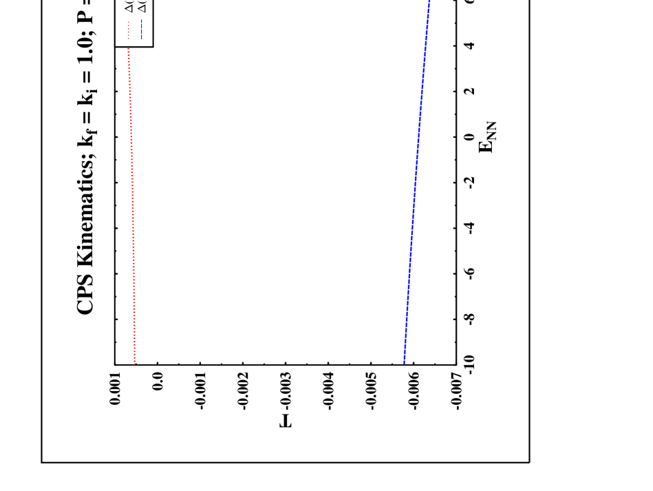
Figure 3: Fractional deviation of approximate $T$ matrix compared to exact evaluation of Eq. (53) using the CPS method, as a function of the 2-body energy (MeV) in the 3-body CM frame. Dotted line uses approximate value described in the text. Dashed line uses the nonrelativistic value.

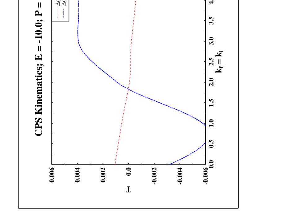
Figure 4: Fractional deviation of approximate $T$ matrix compared to exact evaluation of Eq. (53) using the CPS method, as a function of the 2-body relative momentum (fm^-1), initial and final momenta kept equal. Dotted line uses approximate value described in the text. Dashed line uses the nonrelativistic value.

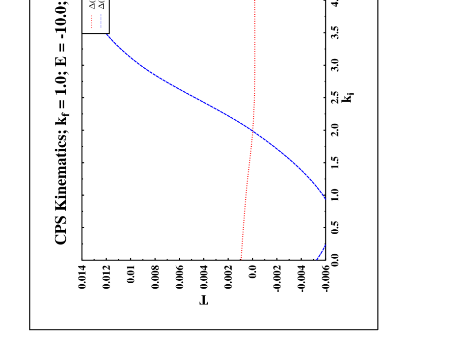
Figure 5: Fractional deviation of approximate $T$ matrix compared to exact evaluation of Eq. (53) using the CPS method, as a function of the 2-body initial relative momentum (fm^-1). Dotted line uses approximate value described in the text. Dashed line uses the nonrelativistic value.

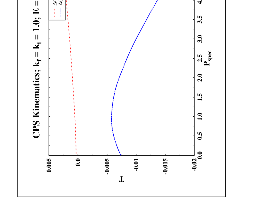
Figure 6: Fractional deviation of approximate $T$ matrix compared to exact evaluation of Eq. (53) using the CPS method, as a function of the spectator momentum (fm^-1). Dotted line uses approximate value described in the text. Dashed line uses the nonrelativistic value.

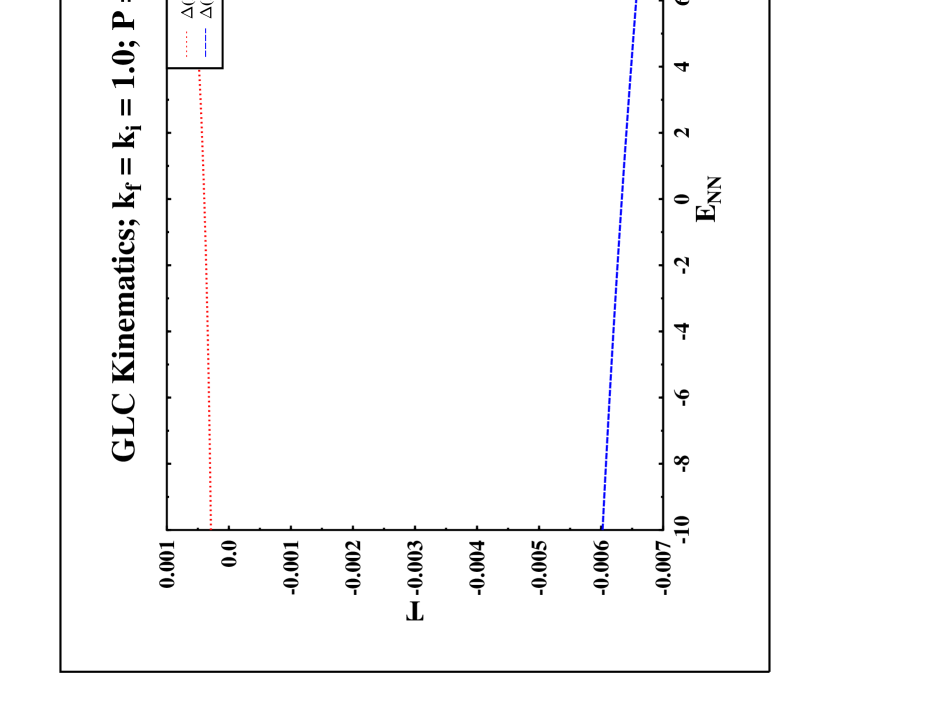
Figure 7: Same as Fig. 3 except using the GLC method.

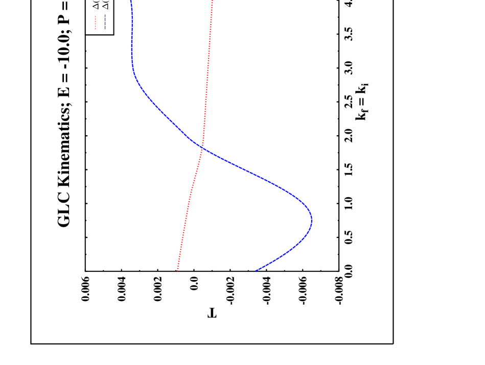
Figure 8: Same as Fig. 4 except using the GLC method.

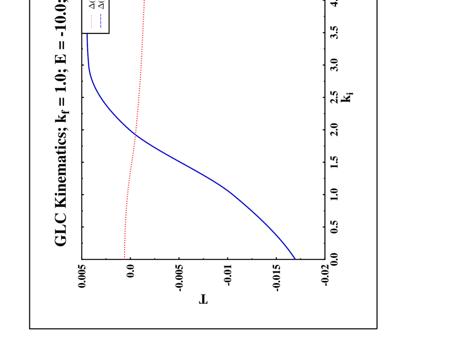
Figure 9: Same as Fig. 5 except using the GLC method.

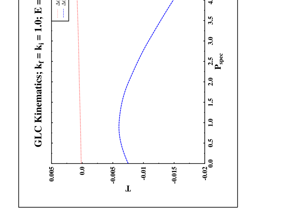
Figure 10: Same as Fig. 6 except using the GLC method.

Figure 11: Same as Fig. 3 except using the GK method.

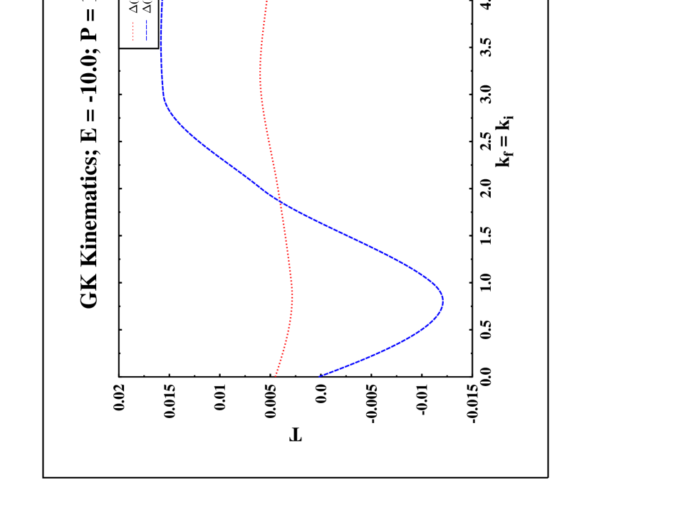
Figure 12: Same as Fig. 4 except using the GK method.

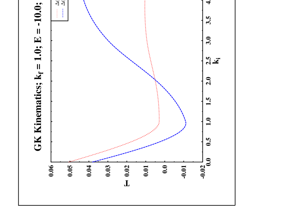
Figure 13: Same as Fig. 5 except using the GK method.

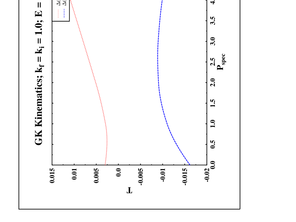
Figure 14: Same as Fig. 6 except using the GK method.

The other factor that appears in a full relativistic three body calculation are the three body recoupling coefficients. These differ from the non-relativistic coefficients by kinematic factors and the presence of momentum dependent spin rotation functions. In many relativistic calculations the overall contribution of the spin effects have proved to be unimportant, however most of these applications have involved bound states.

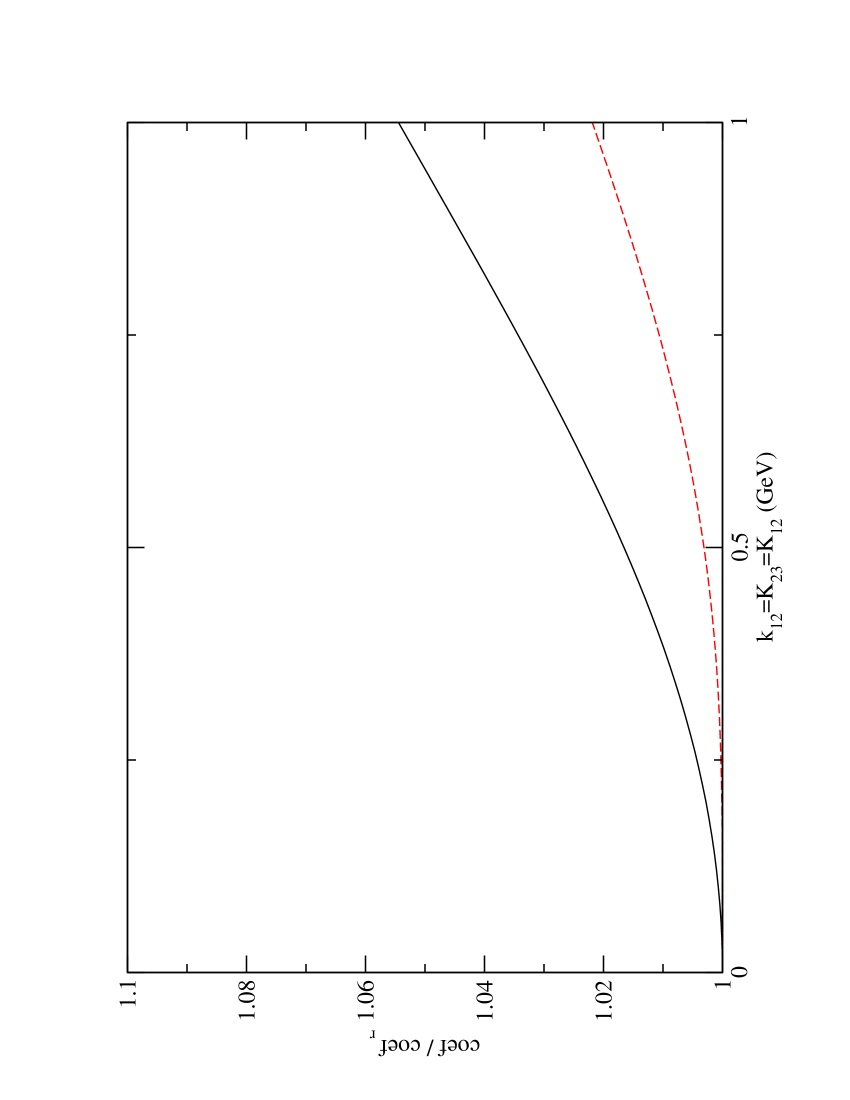
Figure 15: Ratio of the recoupling coefficients.

It is a simple matter to compute relativistic and nonrelativistic recoupling coefficients. To compare them the, delta function in either invariant mass or non-relativistic internal energy is replaced by a delta function in the momentum followed by the appropriate Jacobian factors. The comparison can then be made between the coefficients of the delta functions in the two cases. Figure 15 is typical of the behavior of the recoupling coefficient. The curves are computed for $k_{12}=K_{23}=K_{12}$ for a representative set of spin quantum numbers. The solid curve is the ratio of the non-relativistic to the relativistic recoupling coefficient when they are made to have the same delta function. The dotted curve shows the ratio of relativistic coefficient with the rotation functions turned off to the full relativistic recoupling coefficient.

The curves show that the non-relativistic curve is about 2% higher than the relativistic curve at 0.5 GeV. It grows to just over 5% at 1 GeV. Including the correct multiplicative kinematic factors without including spin rotations leads to considerable improvement at 0.5 GeV; and it grows to just over 2% at 1 GeV. This is consistent with previous calculations that suggest the the recoupling coefficients have small effects.

With the Balian-Brezin method the inclusion of both the spin factors and kinematic factors involve minor modifications to an existing non-relativistic program.

Our conclusion is that negligible errors will be made if the relativistic Faddeev-Lovelace kernel is approximated by replacing the transition matrix elements of $\tilde{T}$ by the expressions in (49),(50), and (51). Care must be used to match the method used to the fitting procedure used to determine the non-relativistic two body interaction. The recoupling coefficients are not needed for calculations dominated by lower momenta; and they lead $5\%$ effects at 1 GeV. The inclusion of the correct kinematic factors reduces errors considerably.

VI Comparison to Approaches Based On Quasipotential Theory

The development and the results discussed above utilize Wigner’s formulation of relativistic quantum mechanics, using a direct construction of a unitary representation of the Poincaré group on the two-nucleon Hilbert space Wigner (1939). The two-nucleon interactions have specific connections both to the Schrödinger equation and to the three-nucleon problem. One can also approach these problems within the framework of a quasipotential theory. The first results for three-nucleon binding were obtained by Stadler and Gross Stadler and Gross (1997), using the so-called spectator approximation Gross (1969, 1974, 1982). Within this framework they can obtain the observed triton binding while maintaining a fit to the observed nucleon-nucleon phase shifts and the deuteron binding. When they compare the results of their “full” calculation to a nonrelativistic approximation, they find that most of the new effects come from the inclusion of negative-energy states. These would correspond approximately to three-nucleon interactions in Poincaré invariant quantum theory. They also find that so-called “boost effects” in their framework are small and give a repulsive contribution to the triton binding. Those results are consistent with the results obtained in Poincaré invariant quantum theory.

An earlier work by Sammarruca and Machleidt Sammarruca and Machleidt (1998) examined the effect of kinematic factors within frameworks based on field theories. They made use of an earlier relation obtained by Brown, Jackson and Kuo Brown et al. (1969), who used quasipotential methods to argue that the non-relativistic interaction should include non-localities. The Brown, Jackson, Kuo method leads to a modified interaction, however unlike the methods discussed above the new interaction must be refit to the phase shift data. This method leads to the following relation between their minimal relativistic and nonrelativistic $t$ matrices:

$$t_{R}({\bf k}^{\prime}\,{\bf k})=\sqrt{\omega_{k}^{\prime}\over m}t_{NR}({\bf k}^{\prime}\,{\bf k})\sqrt{\omega_{k}\over m}.$$ (61)

Sammarruca and Machleidt then use this modified two-nucleon interaction within their relativistic framework and get a net attractive correction to ³H binding when using this factor. Again, this is understandable at least naively when considering that the $t$ matrices receive essentially the opposite factor from those discussed above [Eqs. 49-51]. However, both the Brown, Jackson and Kuo method and the CGL method in principle require a refitting of the phase shifts to get an exact phase equivalence. Thus we cannot make a direct comparison to these methods.

VII Conclusion

We have explored here the quantitative impact of the requirement of relativistic invariance with the framework of Poincaré invariant quantum mechanics. In the range of models discussed here, the dominant effects are manifested in kinematic terms that can easily be incorporated into a Schrödinger-based momentum-space calculation, namely, multiplicative factors of the $E/m$ form, and energy denominators that employ the relativistic energy-momentum relation. There are additional small effects that come from relativistic corrections to the recoupling coefficients. These can be minimized by including the correct relativistic kinematic factors. A correct treatment of these terms involves only minimal modifications of the non-relativistic recoupling coefficients. Quantitatively the effects of all of these corrections are small, and contribute repulsive corrections to three-nucleon binding. This means that the resolution of the discrepancy between Poincaré invariant three-nucleon calculations and the experimentally observed binding energies must come from three-nucleon forces. The quantitative relativistic effects grow with internal momenta; non-relativistic three-nucleon scattering calculations at energies of several hundred MeV may well require corrections beyond the simple square-root factors.