Description of the Nuclear Octupole and Quadrupole Deformation

Description of the Nuclear Octupole and Quadrupole DeformationP.G. Bizzeti, A.M. Bizzeti–Sona

1,2, A.M. Bizzeti–Sona1,2

1

2

A parametrization of octupole plus quadrupole deformation, in terms of intrinsic variables defined in the rest frame of the overall tensor of inertia, is presented and discussed. The model is valid for situations close to the axial symmetry, but non axial deformation parameters are not frozen to zero. The properties of the octupole excitations in the deformed Thorium isotopes ²²⁶Th, ²²⁸Th are interpreted in the frame of this model. A tentative interpretation of octupole oscillations in nuclei close to the X(5) symmetry, in terms of an exactly separable potential, is also discussed.

1 Introduction

We present here a formalism to describe the simultaneous octupole and quadrupole deformations of the nuclear surface, close to but not coincident with the axial symmetry limit, in the frame of Bohr hydrodynamical model. This scheme has been developed in order to discuss phase–transition phenomena in the octupole degree of freedom, a subject which – as it will be explained in the following Section 2 – appeared as a natural development of the experimental and theoretical researches of the group of Florence in the recent years.

Sections  3 and  4 describe the basis of this model and its application to the phase transition between octupole oscillations around a permanently deformed reflection–symmetric shape and rigid rotation of a reflection–asymmetric rotor. These parts summarize the results contained in a recent paper in the Physical Review C [1]. Finally, some new results are reported in the Section 5, while in Section 6 a simple model, based on a separable potential, is discussed and used to tentatively interpret the octupole oscillations in nuclei close to the X(5) critical point.

2 Some history

Our interest on the octupole excitations dates at least from the late ’90s, when we have searched and found evidence for two–octupole–phonon excitations in ¹⁴⁴Nd and ¹⁴⁶Sm [2] and we have long searched, but not found, three–octupole–phonon excitations in ¹⁴⁸Gd [3].

Later, we have been impressed by Iachello results [4, 5] on the symmetries at the critical point, such as E(5) and X(5) (other symmetries, like Y(5) and Z(5), have been proposed later [6, 7]). The first example of X(5) symmetry was identified in ¹⁵²Sm [8], a well known transitional nucleus. We had some experience of another transitional region, that of Mo and Tc isotopes: so, we could identify another possible X(5) candidate [9] in the ¹⁰⁴Mo isotope . We also observed that the X(5) model was able to account for not only the ground–state band, but also the excited $\gamma$ bands, both in ¹⁰⁴Mo and in ¹⁵²Sm. This fact is not trivial, because the negative parity bands, present at low excitation in ¹⁵²Sm, show a very different behaviour. We shall come back to this point in the following.

We also noted some regularities in the proton and neutron numbers of these two X(5) nuclei. In fact, ¹⁰⁴Mo has $Z=42,\ N=62$, ¹⁵²Sm has $Z=62,\ N=90$: one could suspect that another phase transition takes place also for $Z\approx 90$.

Actually, the standard indicators of quadrupole collectivity, and in particular the ratio $R_{2}=E(4^{+})/E(2^{+})$ give indication of a phase transition in the Ra ($Z=88$) and Th ($Z=90$) isotopic chains. Heavier isotopes have rotational character, while the lighter ones appear to be vibrational (or non collective). Moreover, the energies of positive parity levels in the ground–state band of ²²⁴Th and ²²⁴Ra show an impressive agreement with the predictions of the X(5) model [10, 11]. However, in addition to the positive parity band, these nuclei possess a odd-$J$, negative parity band which starts with a $1^{-}$ level lying slightly above the $2^{+}$ and merges with the positive–parity one at $J\approx 5$ or 6. This means that octupole degrees of freedom are important in these nuclei, and their effect must be considered when the evolution of the nuclear shape is followed along the isotopic chain. We observe that ²³⁰Th and heavier isotopes of Th give evidence of octupole vibrations combined with the rotation of a deformed (but reflection symmetric) core: rotational–like bands are built over the one–octupole–phonon states with different values of $K$ (the angular–momentum component along the approximate symmetry axis). In lighter isotopes, the excitation energy of the $1^{-}$ band head of the $K^{\pi}=0^{-}$ band decreases well below those of the other octupole bands, and approaches the rotational–energy value. Eventually, one observes an alternate–parity band which approaches (but never reaches) the behaviour of a rigid, rotation asymmetric rotor, typical of binary asymmetric molecules. In conclusion, a phase transition for the octupole degrees of freedom seems to take place in the Th and Ra isotopes, not far from the critical point of the quadrupole one, but in the opposite direction: with octupole vibration where the quadrupole deformation is stable, and vice-versa. We can also observe that only the $K^{\pi}=0^{-}$ band seems to change substantially along the isotopic chain. This means that the relevant quadrupole and octupole degrees of freedom are those related to axially symmetric, or quasi–axially–symmetric, deformations.

At this point, one needs a theoretical scheme able to describe the evolution of quadrupole and octupole deformations, close to the axial symmetry, across the critical point of the phase transition.

In the frame of the algebraic approach, new developments of the Interacting Vector Boson Model have been reported at this workshop [13]. The $spdf$ extension of the IBM [14] is also able to account for negative–parity excitations. This model, however, is not the most suitable to describe the phase transitions.

In the frame of the geometrical approach, the most complete treatment is the one proposed by Donner and Greiner [15]. They use the Bohr intrinsic frame, defined by the symmetry axes of the quadrupole, and refer to this frame the seven amplitudes of the octupole mode (the overall tensor of inertia being not diagonal in this reference frame). This approach, however, is useful only when all the octupole amplitudes are small compared to the quadrupole deformation. Other models [16, 17, 18] frozen to zero part of the dynamical variables, and are usually limited to the axially symmetric case: what is probably enough in the presence of a stable quadrupole deformation, but not necessarily when the quadrupole deformation approaches zero.

Finally, we have noted a very interesting work by Wexler and Dussel [19], which shows that it is possible to define an intrinsic reference frame for the octupole mode, in which the tensor of inertia is diagonal. In this frame, the seven octupole amplitudes can be parametrized in terms of four intrinsic variables (as the five quadrupole amplitudes are parametrized in term of $\beta_{2}$ and $\gamma_{2}$ in the Bohr representation). This approach, however, is valid for the octupole mode alone.

In conclusion: in order to describe quadrupole and octupole deformation, close to but not coincident with the axial symmetry and with the octupole amplitude not necessarily small compared with the quadrupole one, we were obliged to introduce our own parametrization scheme.

3 The basis of the model

We must start, as usual, from the definition of the nuclear surface in polar coordinates, in the laboratory frame:

$$r(\theta,\phi)=R_{0}\Big{[}1+\!\sum_{\lambda=2,3}\phantom{mj}\sum_{\phantom{m}\mu=-\lambda,\lambda}\alpha^{(\lambda)}_{\mu}Y^{*}_{\lambda,\mu}(\theta,\phi)\Big{]},\hskip 19.91692pt\alpha^{(\lambda)}_{-\mu}=(-)^{\mu}{\alpha_{\mu}^{(\lambda)}}^{*}$$ (1)

We limit our model space to quadrupole and octupole, and we assume that the deformation is small enough not to need to introduce a monopole or dipole term to keep constant the nuclear volume and the center–of–mass position. For the expression of the kinetic energy, we use that of the Bohr hydrodynamical model, $T=\frac{1}{2}\sum_{\lambda}B_{\lambda}\sum_{\mu}|\dot{\alpha}^{(\lambda)}_{\mu}|^{2}\ .$ Then, the laboratory amplitudes $\alpha^{(\lambda)}_{\mu}$ are expressed in terms of the corresponding amplitudes in a proper intrinsic frame and of the Euler angles $\theta_{1},\ \theta_{2},\ \theta_{3}$ defining the orientation of the intrinsic frame in the lab,

$$\sqrt{B_{\lambda}}\ \alpha^{(\lambda)}_{\mu}=\sum_{\nu}a^{(\lambda)}_{\nu}{D^{(\lambda)}_{\mu\nu}}^{*}(\theta_{i})$$ (2)

where the $D^{(\lambda)}$ are Wigner matrices. Note that, in order to simplify the notations, the inertia parameter $B_{\lambda}$ has been included in our definition of $a^{(\lambda)}$. In terms of the new variables, the expression of the kinetic energy splits in three parts: a vibrational term $T_{\rm vib}=\frac{1}{2}\sum_{\lambda,\mu}|\dot{a}^{(\lambda)}_{\mu}|^{2}$; a rotational term $T_{\rm rot}=\frac{1}{2}\sum_{k,k^{\prime}}{\mathcal{J}_{kk^{\prime}}}q_{k}q_{k^{\prime}}$, quadratic in the intrinsic components $q_{k}$ of the angular velocity; and a coupling term $T_{\rm coup}$, not present in the Bohr model for quadrupole motion: $T_{\rm coup}=i\sqrt{21}\ [q^{(1)}\otimes[a^{(3)}\otimes\dot{a}^{(3)}]^{(1)}]^{(0)}_{0}$. For the non diagonal components of the tensor of inertia, the hydrodynamical model gives

$${\mathcal{J}_{13}}\! {+} \!{i\ \mathcal{J}_{23}}\ =\ \sum_{\lambda}{C_{2}(\lambda)}\ \left[a^{(\lambda)}\otimes a^{(\lambda)}\right]^{(2)}_{1}$$ (3)

$${\mathcal{J}_{23}}\! = \!\sum_{\lambda}{C_{2}(\lambda)}\ {\rm Im}\left[a^{(\lambda)}\otimes a^{(\lambda)}\right]^{(2)}_{2}$$ (4)

where $C_{2}(2)=-\sqrt{21}$, $C_{2}(3)=\sqrt{126}$. It is relatively easy to find a parametrization which automatically sets to zero the non-diagonal products of inertia, as far as quadrupole and octupole are treated separately. For the quadrupole, it is the classical one by Bohr, $a^{(2)}_{0}=\beta_{2}\cos\gamma_{2}$, $a^{(2)}_{1}=0$ $a^{(2)}_{2}=\sqrt{1/2}\ \beta_{2}\ \sin\gamma_{2}$. For the octupole, we assume a parametrization similar to that of Wexler and Dussel [19]:

$$a^{(3)}_{0} = \beta_{3}\ \cos\gamma_{3}$$ (5)

$$a^{(3)}_{1} = -(5/2)\ \left(X+iY\right)\ \sin\gamma_{3}$$ (6)

$$a^{(3)}_{2} = \sqrt{1/2}\ \beta_{3}\ \sin\gamma_{3}$$ (7)

$$a^{(3)}_{3} = X\left[\cos\gamma_{3}+(\sqrt{15}/2)\ \sin\gamma_{3}\right]+i\ Y\left[\cos\gamma_{3}-(\sqrt{15}/2)\ \sin\gamma_{3}\right]\ .$$

In both cases, the $a^{(\lambda)}_{\mu}$ amplitudes with $|\mu|=2$ are real, while the $|\mu|=1$ terms are either zero or small of the second order, if we consider small of the first order the other non-axial amplitudes.

The problem arises when both quadrupole and octupole terms are present, since the principal axes of the quadrupole and of the octupole tensor of inertia do not necessarily coincide.

We want to use, as in the Bohr model, an intrinsic frame defined by the principal axes of the tensor of inertia. We must therefore impose the conditions ${\cal J}_{ij}=0$ for $i\neq j$. This is a set of 3 non linear equations, but we can linearize them if we assume that non axial amplitudes are small in comparison with the axial ones. One obtains, up to the first order in the small amplitudes,

$$\mathcal{J}_{12} = -2\sqrt{6}\left(\beta_{2}{\rm Im}\ a^{(2)}_{2}+\sqrt{5}\ \beta_{3}{\rm Im}\ a^{(3)}_{2}\right)=0$$ (8)

$$\mathcal{J}_{13} + i\mathcal{J}_{23}\ =\ \sqrt{6}\ \left(\beta_{2}a^{(2)}_{1}+\sqrt{2}\ \beta_{3}a^{(3)}_{1}\right)=0$$ (9)

which are automatically verified if we put

$$\begin{array}[c]{lp{0.1mm}lp{0mm}l}a^{(2)}_{1}=-c_{1}\sqrt{2}\ \beta_{3}\left(\eta_{c}+i\zeta_{c}\right)&&a^{(3)}_{1}=c_{1}\beta_{2}\left(\eta_{c}+i\zeta_{c}\right)\\[8.0pt] {\rm Im}\;a^{(2)}_{2}=-c_{2}\sqrt{5}\ \xi_{c}&&{\rm Im}\;a^{(3)}_{2}=c_{2}\beta_{2}\ \xi_{c}\end{array}$$ (10)

with the new parameters $\eta_{c},\ \zeta_{c}$ and $\xi_{c}$ small of the first order. The factors $c_{1}$, $c_{2}$ are – at the moment – arbitrary functions of $\beta_{2}$ and $\beta_{3}$.

Now, we can introduce the matrix of inertia $\cal G$, which relates the classical kinetic energy to the components $u_{i}$ of the generalized velocity vector:

$$T=\frac{1}{2}\sum{\cal G}_{ik}u_{i}u_{k}$$ (11)

where, in our case, $u=\{\dot{\beta}_{2},\ \dot{\gamma}_{2},\ \dot{\beta}_{3},\ \dot{\gamma}_{3},\ \dot{X},\ \dot{Y},\ \dot{\xi},\ \dot{\eta},\ \dot{\zeta},\ q_{1},\ q_{2},\ q_{3}\}$. The matrix $\cal G$ and its determinant $G$ play an important role in the quantization of the kinetic energy, according to the Pauli procedure [20].

If we want that the results of the Bohr model be obtained at the limit of $\beta_{3}\ll\beta_{2}$, we must verify that this happens, first of all, for the determinant $G$. Now, the simplest possible choice of constant factors $c_{1}$ ad $c_{2}$ in the Eq. 10 would give $G\propto\beta_{2}^{14}$, while in the Bohr model it should be $\propto\beta_{2}^{8}$. A better choice would be

$$c_{1}=(\beta_{2}^{2}+2\beta_{3}^{2})^{-1/2}\phantom{mmm}c_{2}=(\beta_{2}^{2}+5\beta_{3}^{2})^{-1/2}$$ (12)

With this choice, $G$ has the correct limit when $\beta_{3}\rightarrow 0$. Moreover, all non diagonal elements of $\cal G$ involving either $\beta_{2}$ or $\beta_{3}$ and one of the derivative of the other intrinsic amplitudes or $q_{3}$ are exactly zero. Other non diagonal elements are small at least of the first order and it is possible to show [1] that they have negligible effects, apart from the elements of the last line and column. The latter, in fact, are also small of the first order, but must be compared with the diagonal element ${\cal J}_{3}$, which is small of the second order.

Table 1: The matrix of inertia $\mathcal{G}$: leading terms and relevant first-order terms. Other first-order terms are indicated with the symbol $\approx\!0$. Here $\gamma=\sqrt{5}\gamma_{2}\!-\!\gamma_{3}$, $\mathcal{J}_{1}=3(\beta_{2}^{2}+2\beta_{3}^{2})+2\sqrt{3}(\beta_{2}^{2}\gamma_{2}+\sqrt{5}\beta_{3}^{2}\gamma_{3})$; $\mathcal{J}_{2}=3(\beta_{2}^{2}+2\beta_{3}^{2})-2\sqrt{3}(\beta_{2}^{2}\gamma_{2}+\sqrt{5}\beta_{3}^{2}\gamma_{3})$; and $\mathcal{J}_{3}=4(\beta_{2}^{2}\gamma_{2}^{2}+\beta_{3}^{2}\gamma_{3}^{2})+18(X^{2}+Y^{2})+2(\eta^{2}+\zeta^{2})+8\xi^{2}$.

	$\dot{\beta_{2}}$	$\dot{\gamma_{2}}$	$\dot{\beta_{3}}$	$\dot{\gamma_{3}}$	$\dot{X}$	$\dot{Y}$	$\dot{\xi}$	$\dot{\eta}$	$\dot{\zeta}$	$q_{1}$	$q_{2}$	$q_{3}$
$\dot{\beta_{2}}$	1	0	0	0	0	0	0	0	0	$\approx\!0$	$\approx\!0$	0
$\dot{\gamma_{2}}$	0	$\beta_{2}^{2}$	0	0	0	0	0	0	0	$\approx\!0$	$\approx\!0$	$\frac{-\!\sqrt{40}\beta_{2}\beta_{3}\xi}{\sqrt{\beta_{2}^{2}+5\beta_{3}^{2}}}$
$\dot{\beta}_{3}$	0	0	1	0	0	0	0	0	0	$\approx\!0$	$\approx\!0$	0
$\dot{\gamma_{3}}$	0	0	0	$\beta_{3}^{2}$	$\approx\!0$	$\approx\!0$	0	$\approx\!0$	$\approx\!0$	$\approx\!0$	$\approx\!0$	$\frac{\sqrt{8}\beta_{2}\beta_{3}\xi}{\sqrt{\beta_{2}^{2}+5\beta_{3}^{2}}}$
$\dot{X}$	0	0	0	$\approx\!0$	2	0	0	$\approx\!0$	0	$\approx\!0$	$\approx\!0$	$6Y$
$\dot{Y}$	0	0	0	$\approx\!0$	0	2	0	0	$\approx\!0$	$\approx\!0$	$\approx\!0$	$-\!6X$
$\dot{\xi}$	0	0	0	0	0	0	2	0	0	$\approx\!0$	$\approx\!0$	$\frac{\sqrt{8}\beta_{2}\beta_{3}\gamma}{\sqrt{\beta_{2}^{2}+5\beta_{3}^{2}}}\phantom{.}$
$\dot{\eta}$	0	0	0	$\approx\!0$	$\approx\!0$	0	0	2	0	$\approx\!0$	$\approx 0$	$2\zeta$.
$\dot{\zeta}$	0	0	0	$\approx\!0$	0	$\approx\!0$	0	0	2	$\approx\!0$	$\approx\!0$	$-2\eta$
$q_{1}$	$\approx\!0$	$\approx\!0$	$\approx\!0$	$\approx\!0$	$\approx\!0$	$\approx\!0$	$\approx\!0$	$\approx\!0$	$\approx\!0$	${\mathcal{J}_{1}}$	0	0
$q_{2}$	$\approx\!0$	$\approx\!0$	$\approx\!0$	$\approx\!0$	$\approx\!0$	$\approx\!0$	$\approx\!0$	$\approx\!0$	$\approx\!0$	0	${\mathcal{J}_{2}}$	0
$q_{3}$	0	$[..]$	0	$[..]$	$6Y$	$-\!6X$	$[..]$	$2\zeta$.	$-2\eta$	0	0	$\mathcal{J}_{3}$

Relevant terms of the matrix $\cal G$ are shown in the Table 1. It can be observed that the variables $\gamma_{2}$ and $\gamma_{3}$ appear only in the combination $\gamma=\sqrt{5}\ \gamma_{2}-\gamma_{3}$. In the place of $\gamma_{2}$ and $\gamma_{3}$ it will be convenient to use the new variable $\gamma$ and the orthogonal combination $\gamma_{0}\!=\!c_{0}\ (\beta_{2}^{2}\gamma_{2}+\sqrt{5}\beta_{3}^{2}\gamma_{3})$, entering in the expression of $G$. Once more, the factor $c_{0}$ is – at the moment – an arbitrary function of $\beta_{2}$ and $\beta_{3}$. We can observe that $\gamma_{0}$ is a measure of the triaxiality of the overall tensor of inertia. In fact, if $\gamma_{0}=0$, ${\cal J}_{1}={\cal J}_{2}$ (apart from terms of the second order) and the tensor of inertia is axially symmetric, even if the nuclear surface is not. In some way, $\gamma_{0}$ plays a role similar to that of $\gamma_{2}$ in the pure quadrupole case.

Now, to characterize the different degrees of freedom with respect to the angular momentum projection $L_{3}$ and to the parity, it is convenient to perform another change of representation:

$$X = w\sin\vartheta\phantom{mmmj}Y\ =\ w\cos\vartheta$$

$$\eta = v\sin\varphi\phantom{mmmm}\zeta\ =\ v\cos\varphi$$ (13)

$$\xi = u\sin\chi\phantom{mmmm}\gamma\ =\ \sqrt{2}\ \left(\sqrt{\beta_{2}^{2}+5\beta_{3}^{2}}\ /\ \beta_{2}\beta_{3}\right)u\cos\chi$$ (14)

$$\frac{\gamma_{0}}{c_{0}} = f_{0}(\beta_{2},\beta_{3})\ u_{0}$$ (15)

Choosing $f_{0}(\beta_{2},\beta_{3})=\sqrt{\beta_{2}^{2}+5\beta_{3}^{2}}$ one obtains for the determinant of $\mathcal{G}$

$$G={\rm Det}\;\mathcal{G}=2304\ \big{(}\beta_{2}^{2}+2\beta_{3}^{2}\big{)}^{2}\ u_{0}^{2}\ v^{2}\ u^{2}\ w^{2}\ .$$ (16)

At this point, the matrix of inertia takes a very simple form. The relevant non-diagonal terms are limited to the small sub-matrix involving $q_{3}$ and the time derivatives of $\varphi,\ \chi$ and $\vartheta$, which can be diagonalized easily. To this purpose, we evaluate the intrinsic angular momentum component $L_{3}=\partial T/\partial q_{3}$ and also the conjugate moments $p_{\varphi},\ p_{\chi},\ p_{\vartheta}$ of the angular variables $\varphi,\ \chi,\ \vartheta$:

$$p_{\varphi} = 2v^{2}\ (\dot{\varphi}+q_{3})$$

$$p_{\chi} = 2u^{2}\ \left(\dot{\chi}+2q_{3}\right)$$ (17)

$$p_{\vartheta} = 2w^{2}\ (\dot{\vartheta}+3q_{3})\ .$$

$$L_{3} = \mathcal{J}_{3}q_{3}+\left[2v^{2}\dot{\varphi}+4u^{2}\dot{\chi}+6w^{2}\dot{\vartheta}\right]$$ (18)

$$= (p_{\varphi}+2p_{\chi}+3p_{\vartheta})\ +\ 4u_{0}^{2}q_{3}\ .$$

One can immediately observe that when $u_{0}=0$ (i.e. when ${\cal J}_{1}={\cal J}_{2}$), $q_{3}\rightarrow\infty$ unless $L_{3}=\Omega\equiv p_{\varphi}+2p_{\chi}+3p_{\vartheta}$. This means that $\Omega$ is the component of the intrinsic angular momentum along the axis 3, which survives also if this is an axial–symmetry axis for the overall tensor of inertia. If we assume that the potential energy does not depend on $\varphi,\ \chi,$ or $\vartheta$, it is easy to realize that $p_{\varphi},\ p_{\chi}$ and $p_{\vartheta}$ are quantized and are integer multiples of $\hbar$: the degrees of freedom corresponding to the pairs of variables $(v,\ \varphi),\ (u,\ \chi),\ (w,\ \vartheta)$ correspond to 1, 2 and 3 units of angular momentum along the intrinsic axis 3. This is obvious in the latter case, which concerns the octupole variables $a^{(3)}_{\pm 3}$, but not for the other two, in which quadrupole and octupole variables are mixed together. It is also possible to show [1] that these variables carry negative parity.

It remains to consider the variable $u_{0}$. If we assume that the differential equation for $u_{0}$ can be decoupled from the others, this equation takes the form

$$\left\{\frac{1}{u_{0}}\frac{\partial}{\partial u_{0}}\left[u_{0}\frac{\partial}{\partial u_{0}}\right]+\frac{2}{\hbar^{2}}\left[E_{u_{0}}-U(u_{0})\right]-\ \frac{1}{u_{0}^{2}}\left[\frac{K_{0}}{2}\right]^{2}\right\}\phi(u_{0})=0$$ (19)

where we have put $K_{0}=L_{3}-\Omega$. The variable $u_{0}$ can take positive as well as negative values. The condition of continuity for the wavefunction $\phi(u_{0})$ and its derivative at $u_{0}=0$ imposes that $K_{0}=2n_{u_{0}}$, with $n_{u_{0}}$ integer. We can conclude that the degree of freedom associated to the variable $u_{0}$ carries two units of angular momentum along the intrinsic axis 3, and it is possible to show that it carries positive parity. The inverse of the matrix $\cal G$ turns out to be diagonal (at the relevant order) in the space of momenta conjugate to the variables defined in the Eq. 15 and of the angular momentum components $L_{1}$, $L_{2}$ and $K_{0}$. The Table 2 shows a more general form of this matrix, with the variable $u_{0}$ replaced by $\gamma_{0}=u_{0}/R(\beta_{2},\beta_{3})$, where $R=1/[c_{0}(\beta_{2},\beta_{3})f_{0}(\beta_{2},\beta_{3})]$  (see Eq. 15). A more formal derivation of these results, involving the derivatives of the Euler angles, can be found in the Appendix C of ref. [1].

Table 2: The matrix ${\cal G}^{-1}$ in the space of momenta (only the leading terms are shown). Here, $K_{0}=L_{3}-\Omega$, with $\Omega=p_{\varphi}+2p_{\chi}+3p_{\vartheta}$, and $\gamma_{0}=u_{0}/R$.

	$\partial/\partial{\beta}$	$\partial/\partial{\delta}$	$\partial/\partial{\gamma_{0}}$	$\partial/\partial{v}$	$\partial/\partial{u}$	$\partial/\partial{w}$	$\partial/\partial{\varphi}$	$\partial/\partial{\chi}$	$\partial/\partial{\vartheta}$	$L_{1}$	$L_{2}$	$K_{0}$
$\partial/\partial{\beta}$	1	0	0	0	0	0	0	0	0	0	0	0
$\partial/\partial{\delta}$	0	$\frac{1}{\beta^{2}}$	0	0	0	0	0	0	0	0	0	0
$\partial/\partial{\gamma_{0}}$	0	0	$\frac{1}{R^{2}}$	0	0	0	0	0	0	0	0	0
$\partial/\partial{v}$	0	0	0	$\frac{1}{2}$	0	0	0	0	0	0	0	0
$\partial/\partial{u}$	0	0	0	0	$\frac{1}{2}$	0	0	0	0	0	0	0
$\partial/\partial{w}$	0	0	0	0	0	$\frac{1}{2}$	0	0	0	0	0	0
$\partial/\partial{\varphi}$	0	0	0	0	0	0	$\frac{1}{2v^{2}}$	0	0	0	0	0
$\partial/\partial{\chi}$	0	0	0	0	0	0	0	$\frac{1}{2u^{2}}$	0	0	0	0
$\partial/\partial{\vartheta}$	0	0	0	0	0	0	0	0	$\frac{1}{2w^{2}}$	0	0	0
$L_{1}$	0	0	0	0	0	0	0	0		$\frac{1}{{\cal J}_{1}}$	0	0
$L_{2}$	0	0	0	0	0	0	0	0	0	0	$\frac{1}{{\cal J}_{2}}$	0
$K_{0}$	0	0	0	0	0	0	0	0	0	0	0	$\frac{1}{R^{2}\gamma_{0}^{2}}$

4 The axial octupole mode with stable quadrupole deformation

This is the simplest case in which the properties of octupole excitation can be followed from the limit of harmonic oscillations around the reflection symmetric core to the opposite limit of stable octupole deformation. A detailed discussion of this subject can be found in the ref. [1], and a few preliminary results have been reported at two earlier Conferences [10, 11]. Here, we only summarize these results.

A preliminary comment is in order. The properties of the quadrupole vibrations around an axially deformed core are better described [23] with respect to the intrinsic parameters $a^{(2)}_{2}$, $\delta a^{(2)}_{0}=a^{(2)}_{0}-\bar{a}^{(2)}_{0}$ than in terms of the Bohr parameters $\beta_{2}$ and $\gamma_{2}$. We have seen that the parameter $u_{0}$ defined in the eq. 15 plays, in our treatment, a role analogous to that of $a^{(2)}_{2}$ in the pure quadrupole Hamiltonian. It appears reasonable, therefore, to use it as a dynamical variable instead of defining an angle variable similar to the $\gamma_{2}$ of the quadrupole case. Therefore, we can use the form of the matrix ${\cal G}^{-1}$ given in Table 2, with $R=1$, to derive the differential equation for $\beta_{3}$, according to the Pauli prescriptions (in doing this, we assume decoupling of the $\beta_{3}$ motion from the small–amplitude oscillations in all other degrees of freedom). One obtains

$$\frac{{\rm d}^{2}\psi(x)}{{\rm d}x^{2}}+\frac{2x}{1+x^{2}}\frac{{\rm d}\psi(x)}{{\rm d}x}+\left[\epsilon-\frac{J(J+1)}{6(1+x^{2})}-v(x)\right]\psi(x)\!=\!0$$ (20)

where $x=\sqrt{2}\beta_{3}/\bar{\beta}_{2}$, while $v(x),\ \epsilon$ are the potential energy and the energy eigenvalue in a proper energy unit, and $\psi(-x)=(-)^{J}\psi(x)$. As for the potential $v(x)$, we have considered two simple cases: a quadratic expression $v=\frac{1}{2}cx^{2}$ or a critical (square-well) potential, as in the X(5) model: $v(x)=0$ for $|x|<b$ and $=+\infty$ for $|x|>b$. In both cases, the model has one free parameter ($c$ or $b$) to be adjusted to fit the experimental data. In the figure 1 the energies of positive and negative parity levels of ²²⁶Th and ²²⁸Th are compared with different model predictions. The former turns out to be close to the results we obtain for a critical-point potential, while the latter is closer to those obtained with a quadratic potential.

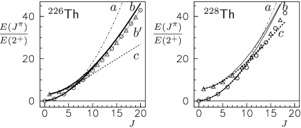
Figure 1: (From ref. [1]). Excitation energies for states of positive parity (circles) and negative parity (triangles), in units of $E(2^{+})$, for the ground-state band of ²²⁶Th and ²²⁸Th. Theoretical curves: $a$ – rigid rotor; $b\ (b^{\prime})$ – present model with critical potential, fitted on the $1^{-}$ state (on the high-spin states); $c$ – present model with harmonic potential.

5 Latest developments

The results reported until now are, apart from some limited extensions, those contained in our recent paper in Physical Review C [1]. From now on, we move to the region where not only $\beta_{3}$ but also $\beta_{2}$ is allowed to vary, in principle down to zero: this is still a partially unexplored land, were work is in progress and results might be subject to change. Eventually, it will be useful to move from the Cartesian representation in terms of $\beta_{2},\ \beta_{3}$ to a polar one, in terms of the new variables $\beta$, $\delta$ with $\beta_{2}=\beta\cos\delta$, $\beta_{3}=\beta\sin\delta$ as in the work by Minkov [21], but for the moment we will continue to use the Cartesian representation.

For consistency with the well established results on the pure quadrupole case, we need that our results converge to those of the Bohr model in the limit of small octupole deformation. As we are going to see, this requirement will put some restrictions on the possible models of octupole plus quadrupole excitations. E.g., the form of the matrix $\cal G$ we have used in the case of permanent quadrupole deformation is not suitable in the present case, as its determinant $G$, at the limit of small $\beta_{3}$, is proportional to $\beta_{2}^{4}$, while it should be proportional to $\beta_{2}^{8}$ according to the Bohr model. It is easy to recognize that the responsibility for the disagreement can be attributed to the choice of $u_{0}$ as a dynamical variable. Since in the Bohr model the variable $\gamma_{2}$ is used in the place of $a^{(2)}_{2}$, it is now necessary to replace $u_{0}$ with an adimensional variable $\gamma_{0}=u_{0}/R$. We could choose now $R=\beta\equiv\sqrt{\beta_{2}^{2}+\beta_{3}^{2}}$, to obtain the correct limit $G\propto\beta_{2}^{8}$ for $\beta_{3}\!\rightarrow 0$. This is somewhat better, but still not enough: the equation for $\beta_{3}$ obtained with the Pauli quantization rule does not converge to the one of Bohr when $\beta_{3}\rightarrow 0$.

In fact, if we only take into account the dynamical variables $\beta_{2}$ and $\beta_{3}$ (assuming that their equations can be approximately separated from that of $\gamma_{0}$, as in Iachello X(5) model, and from all other dynamical variables), we obtain

$$\left\{G^{-1/2}\frac{\partial}{\partial\beta_{2}}\left[G^{1/2}\frac{\partial}{\partial\beta_{2}}\right]\right.+G^{-1/2}\frac{\partial}{\partial\beta_{3}}\left[G^{1/2}\frac{\partial}{\partial\beta_{3}}\right]$$ (21)

$$+\left.\frac{2}{\hbar^{2}}\left[E-V_{0}(\beta_{2},\beta_{3})\right]-\frac{J(J+1)}{3(\beta_{2}^{2}+2\beta_{3}^{2})}\right\}\ \Psi(\beta_{2},\beta_{3}) = 0$$ (22)

This equation can be somewhat simplified with the substitution

$$\Psi(\beta_{2},\beta_{3})=g^{-1/2}\ \Phi(\beta_{2},\beta_{3})$$ (23)

with $g\propto G^{1/2}$, to obtain

$$\bigg{\{}\frac{\partial^{2}}{\partial\beta_{2}^{2}}+\frac{\partial^{2}}{\partial\beta_{3}^{2}}+\frac{2}{\hbar^{2}}\left[E-V_{0}\right]-\frac{J(J+1)}{3(\beta_{2}^{2}+2\beta_{3}^{2})}\ +\ v(\beta_{2},\beta_{3})\bigg{\}}\ \Phi(\beta_{2},\beta_{3})=0$$ (24)

with

$$v(\beta_{2},\beta_{3})=\frac{1}{4g^{2}}\ \left[\left(\frac{\partial g}{\partial\beta_{2}}\right)^{2}+\left(\frac{\partial g}{\partial\beta_{3}}\right)^{2}\right]-\frac{1}{2g}\left[\frac{\partial^{2}g}{\partial\beta_{2}^{2}}+\frac{\partial^{2}g}{\partial\beta_{3}^{2}}\right]$$ (25)

If $R=\beta$, $g=(\beta_{2}^{2}+\beta_{3}^{2})\ (\beta_{2}^{2}+2\beta_{3}^{2})$, and one obtains

$$v(\beta_{2},\beta_{3})=-\frac{5\beta_{2}^{4}+16\beta_{2}^{2}\beta_{3}^{2}+14\beta_{3}^{4}}{(\beta_{2}^{2}+\beta_{3}^{2})\ (\beta_{2}^{2}+\beta_{3}^{2})^{2}}\Rightarrow-\frac{5}{\beta_{2}^{2}}\ \textit{\rm for}\ \beta_{3}\Rightarrow 0$$ (26)

A similar calculation is possible for the pure quadrupole case, starting from the Bohr expression of $G\propto\beta_{2}^{8}$, but the result is $v(\beta_{2})=-2/\beta^{2}$. Even if the limit of $G$ for $\beta_{3}\rightarrow 0$ converge to the corresponding one of the Bohr model, this is not necessarily true for $v$.

However, it is easy to realize that $v(\beta_{2},\beta_{3})$ converges to $v(\beta_{2})$ of the Bohr model if the first and second partial derivatives of $g$ with respect to $\beta_{3}$ tend to zero when $\beta_{3}\rightarrow 0$. A possible choice of variables leading to this result corresponds to keeping $c_{0}=\sqrt{\beta_{2}^{2}+2\beta_{3}^{2}}$ (instead of $\sqrt{\beta_{2}^{2}+5\beta_{3}^{2}}$ ) in the definition of $\gamma_{0}$. In this case one obtains

$$g(\beta_{2},\beta_{3})=\frac{(\beta_{2}^{2}+\beta_{3}^{2})(\beta_{2}^{2}+2\beta_{3}^{2})^{2}}{\beta_{2}^{2}+5\beta_{3}^{2}}\Rightarrow\beta_{2}^{4}\left[1+8\left(\beta_{3}/\ \beta_{2}\right)^{4}+...\right]$$ (27)

and the first and second derivative of $g$ with respect to $\beta_{3}$ vanish for $\beta_{3}\rightarrow 0$.

6 Specific model for quadrupole–octupole oscillations

We now consider the case of simultaneous quadrupole–octupole oscillations, and in particular the quadrupole motion corresponding to the critical point of phase transition described by the X(5) model. At the limit of small amplitude for the octupole oscillations, we should therefore obtain the same results of X(5). The point is that the octupole amplitude must be, at this limit, small compared to the quadrupole amplitude, which, in turn, can become zero. It is convenient, therefore, to use the new variables $\beta$, $\delta$ defined by

$$\beta_{2}=\beta\cos{\delta}\phantom{mmmm}\beta_{3}=\beta\sin{\delta}$$ (28)

and reach the limit by confining $\delta$ to very small values by a proper potential term. It is clear that also the amplitudes $v,\ u,\ w$ must be small compared to $\beta$, as well as $\gamma_{0}$ compared to 1. At the moment, however, we will forget their presence and only discuss the Schrödinger equation involving the variables $\beta,\ \delta$ and the Euler angles. With this ansatz, and assuming that the potential energy has the form $(\hbar^{2}/2)\ V(\beta,\delta)$, for $K=0$ we obtain

$$\Bigg{\{}\frac{1}{g}\frac{\partial}{\partial\beta}\left[g\frac{\partial}{\partial\beta}\right]+\frac{1}{g}\frac{\partial}{\partial\delta}\left[\frac{1}{\beta^{2}}g\frac{\partial}{\partial\delta}\right]+\epsilon-V-\frac{A_{J}}{\beta^{2}(1+\sin^{2}\delta)}\ \Bigg{\}}\ \Psi(\beta,\delta)=0$$ (29)

where $g\propto G^{1/2}\propto\beta^{5}\ [(1+\sin^{2}\delta)^{2}/\ (1+4\sin^{2}\delta)]\ \gamma_{0}\ u_{0}\ v\ u\ w$, $\epsilon=2E/\hbar^{2}$, and $A_{J}=J(J+1)/3$.

The Eq. 29 has a structure very similar to that of the Bohr equation for pure quadrupole motion at the limit close to the axial symmetry, with our parameter $\delta$ in the place of $\gamma_{2}$. In the case of X(5) symmetry, the Bohr equation has been solved [5] by approximate separation of the variables, substituting the factor $1/\beta_{2}^{2}$ with a proper average value in the differential equation for $\gamma_{2}$. It has already been noted, however, that this approach does work for the $\gamma$ excited bands but not for the negative-parity ones [9]. Now we want to explore some alternative procedure which could better account for the experimental data.

It is convenient to exploit the result of Eq.s 23,24,25, to eliminate in the Eq.29 the first–derivative terms, with the substitution

$$\Psi(\beta,\delta)=g^{-1/2}\ \Psi_{0}(\beta,\delta)$$ (30)

giving

$$\Bigg{\{} \frac{\partial^{2}}{\partial\beta^{2}}+\frac{1}{\beta^{2}}\frac{\partial^{2}}{\partial\delta^{2}}+\epsilon-V(\beta,\delta)-\frac{A_{J}}{\beta^{2}(1+\sin^{2}\delta)}$$

$$-\frac{7}{4}\ \frac{1}{\beta^{2}}-\frac{2\sin^{2}\delta\ (25+12\sin^{2}\delta+8\sin^{4}\delta)}{(1+\sin^{2}\delta)(1+4\sin^{2}\delta)^{2}}\ \frac{1}{\beta^{2}}\Bigg{\}}\ \Psi_{0}=0\ .$$

We can separate the potential term in two parts, one of which depends only on $\beta$: $V(\beta,\delta)=V_{0}(\beta)+V_{1}(\delta,\beta)$ and search a solution in the form $\Psi_{0}(\beta,\delta)=\psi(\beta)\Phi(\delta,\beta)$:

$$\frac{1}{\psi} \left[\frac{\rm{d}^{2}\psi}{\rm{d}\beta^{2}}+\left(\epsilon-V_{0}(\beta)-\frac{A_{J}+\frac{7}{4}+A^{\prime}}{\beta^{2}}\right)\psi\right]$$

$$+ \frac{1}{\beta^{2}\Phi}\left[\frac{\partial^{2}\Phi}{\partial\delta^{2}}+\frac{2\beta^{2}}{\psi}\frac{\partial\psi}{\partial\beta}\frac{\partial\Phi}{\partial\beta}+\beta^{2}\frac{\partial^{2}\Phi}{\partial\beta^{2}}+\Bigg{(}A^{\prime}-\beta^{2}\ V_{1}(\delta,\beta)\right.$$

$$+ \left.\frac{A_{J}\sin^{2}\delta}{1+\sin^{2}\delta}-\frac{2\sin^{2}\delta\ (25+12\sin^{2}\delta+8\sin^{4}\delta)}{(1+\sin^{2}\delta)(1+4\sin^{2}\delta)^{2}}\Bigg{)}\Phi\right]=0\ .$$

This equation is exactly separable if $\beta^{2}V_{1}(\delta,\beta)$ does not depend on $\beta$, i.e. $V_{1}(\delta,\beta)=v(\gamma)/\ \beta^{2}$. This class of potentials has been considered, e.g., by Fortunato [24] in his general discussion about the solutions of the Bohr Hamiltonian. We can reasonably suspect that it be not realistic in our case, but a discussion of this simply solvable model can shed light on the general properties of the quadrupole–octupole vibrations and help to identify more realistic solutions. With such a potential, $\Phi=\phi(\delta)$ is a solution of the differential equation

$$\left[\frac{{\rm d}^{2}\!\phi}{{\rm d}\delta^{2}}\!+\!\left(\!A^{\prime}\!-\!v(\delta)\!+\!\frac{A_{J}\sin^{2}\!\delta}{1\!+\!\sin^{2}\!\delta}\!-\!\frac{2\!\sin^{2}\!\delta(25\!+\!12\sin^{2}\!\delta\!+\!8\sin^{4}\!\delta)}{(1\!+\!\sin^{2}\!\delta)(1\!+\!4\sin^{2}\delta)^{2}}\right)\!\phi\right]\!=\!0$$ (33)

We want to explore first the case of small oscillations of $\delta$ around zero. For our discussion, we do not need to specify the exact form of the potential, but, just as an example, we can assume a harmonic restoring force and expand up to the second order the terms in $\sin^{2}\delta$ (whose effect, however, will be negligible at least for not-to-high values of $J$), to obtain the eigenvalues $A^{\prime}_{n}=(2n+1)A^{\prime}_{0}$ and eigenfunctions alternatively even or odd, with parity $(-)^{n}$. Or, as an alternative, one could use a square-well potential $v(\delta)=0$ for $\delta<\delta_{\ell}$ and $=+\infty$ elsewhere, as exemplified in Fig. 3 $a$. Other potentials would give a different spectrum of eigenvalues but, if they have a single minimum at $\delta=0$, the ground state must correspond to a symmetric solution. We indicate with $A^{\prime}_{+}$ the eigenvalue corresponding to the ground state and with $A^{\prime}_{-}$ the one corresponding to the lowest antisymmetric solution. We want that, for even spin and parity, the equation in $\beta$ take the form of that of the X(5) model, i.e., in our notations,

$$\frac{\rm{d}^{2}\psi}{\rm{d}\beta^{2}}+\left(\epsilon-V_{0}(\beta)-\frac{A_{J}+2}{\beta^{2}}\right)\psi=0$$ (34)

Comparison with Eq. 6 shows that this result would be obtained with $A^{\prime}_{0}=1/4$. Actually, it is probably unnecessary to assume that this relation holds. A general problem of all models considering explicitly only part of the overall set of dynamical variables, is the effect of the zero–point energies of the neglected degrees of freedom, which possibly depend on the value of the active model variables. If a phenomenological potential is used for the latter, this potential should already include the zero–point energies of all other degrees of freedom not explicitly taken into account.

Assuming that the positive–parity states must be described by the X(5) Hamiltonian, the following equation in $\beta$ holds for the lowest $K^{\pi}=0^{\pm}$ bands

$$\frac{\rm{d}^{2}\psi}{\rm{d}\beta^{2}}+\left(\epsilon-V_{0}(\beta)-\frac{A_{J}+2+\Delta_{\pi}}{\beta^{2}}\right)\psi=0$$ (35)

We now consider in particular the case of the critical–point potential, $V_{0}=0$ when $\beta$ is in the interval $0-\beta_{0}$ and $V_{0}=+\infty$ elsewhere. As for the parity dependent term $\Delta_{\pi}$, with our assumptions is $\Delta_{+}=0$. For negative parity, the term $\Delta_{-}=A^{\prime}_{-}-A^{\prime}_{+}$ will be considered as an adjustable parameter. With this assumption, the spectrum of eigenvalues is given by

$$\epsilon(s,J,\pi)-\epsilon_{0}=C\ [x(s,J,\pi)]^{2}$$ (36)

with $C$ constant, $x(s,J,\pi)$ the $s^{th}$ zero of the Bessel function $J_{\nu}(x)$ and

$$\nu=\sqrt{J(J+1)/3+9/4+\Delta_{\pi}}$$ (37)

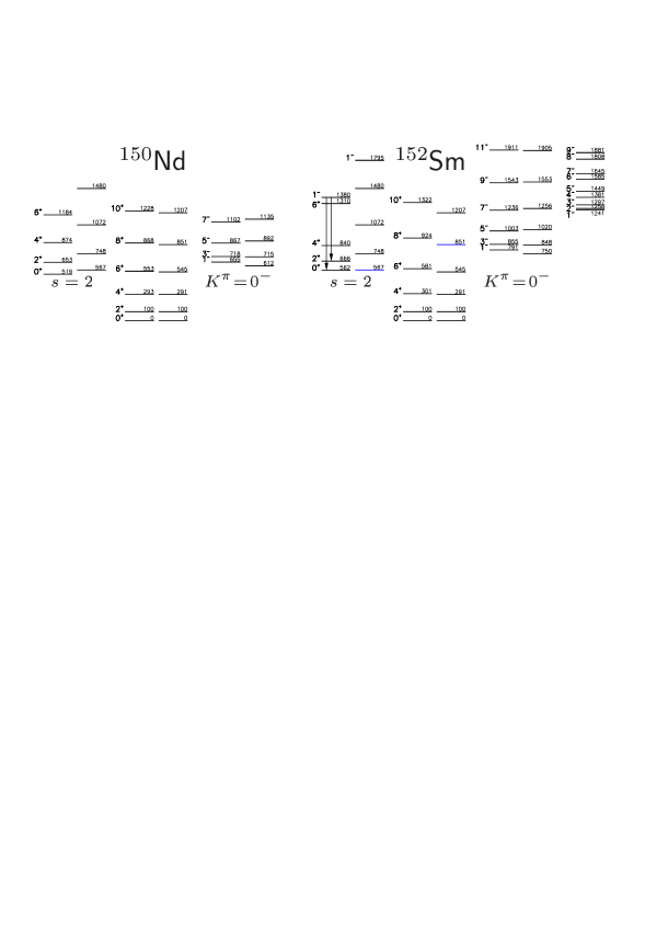
Figure 2: The experimental (left) and theoretical energies (normalized to that of the first excited state) of the $K=0$ bands in ¹⁵⁰Nd and ¹⁵²Sm. In the latter, the experimental values for the $K^{\pi}=1^{-}$ band are also shown. Theoretical values for even $J$ and parity are those of the X(5) model, for odd $J$ and parity are obtained with $\Delta_{-}=15$ for ¹⁵⁰Nd and with $\Delta_{-}=20$ for ¹⁵²Sm.

Fig. 2 shows a partial level scheme of ¹⁵²Sm and ¹⁵⁰Nd, normalized to the energy of the first excited state, and compared with the values derived from Eq. 36 (which, for positive–parity states, coincide with those of the X(5) model). The agreament is fairly good in both cases. In ¹⁵²Sm, the comparison can be extended to the lowest negative–parity state of the $s=2$ band, if the level reported as $1^{(-)}$ really belongs to this band as it would be suggested by its decay. If it is so, its energy is significantly lower than the model prediction, but this happens also for all the $s=2$ excited states of even parity and spin. It must also be noted that in ¹⁵²Sm the odd-$J$ levels of the next octupole band ($K^{\pi}=1^{-}$) seem to mix with those of the lowest one, as indicated by the large odd-even staggering. In the heavier $N=90$ isotones the second octupole band (with $K\neq 0$) gets closer to the first one, and our model is no longer valid in such a case. In well established X(5) nuclei lying in different regions, the lower negative bands seem to be built over intruder states, having a band head $J^{\pi}=3^{-}$ or $5^{-}$.

Is the agreement shown by Fig. 2 a purely accidental one? It is possible, but at least it shows that in this case experimental data can be reproduced by using a separable potential. We shall see that this is not possible in other cases, and in particular in those which seem more interesting to us, ²²⁴Th and ²²⁴Ra.

In these two nuclei, the even $J$, positive parity states follow closely the X(5) model predictions. The negative–parity part of the ground state band lies significantly higher than the positive parity part at low values of $J$, while the two parts merge together above $J\approx 8$. This behaviour is very different from those of the $\gamma$–excited bands in the X(5) nuclei and of the negative parity bands in ¹⁵²Sm and ¹⁵⁰Nd. It could be natural to assume that in these mass-224 nuclei the axial quadrupole and octupole amplitudes do not oscillate independently, but are strictly correlated together: the nuclear deformation oscillates along two symmetric valleys, starting at $\beta=0$ and caracterized by an average value of $\delta$ close to $+\delta_{0}$ or to $-\delta_{0}$. With reference to our Eq.s 28, this means that $\beta$ oscillates in a wide interval, while $\delta$ is confined to a narrow region around some nonzero value. As the potential must be symmetric with respect to $\delta$, this means that possible values of $\delta$ are localized in one of the two regions around $+\delta_{0}$ or $-\delta_{0}$. According to Eq. 33 (with $v(\delta)$ indepentent of $\beta$), this would result in a negligible parity staggering.

In fact, as long as we forget the symmetry of the wavefunction with respect to $\delta$, we find a doubly degenerate spectrum, corresponding to eigenfunction localised either around $+\delta_{0}$ or around $-\delta_{0}$. Reflection symmetry requires that the complete wavefunction be symmetric (the sum of the two) for even values of J and $\pi$, or antisymmetric (their difference) for odd values. As long as the two localized wavefunctions have no overlap (or have a negligible one), the eigenvalues corresponding to even or odd combinations are (almost) equal to those of the localized solutions. The dependence on $J$ of the last-but-one term of Eq. 33 has a minor effect on the results, particularly at low values of $J$. As a consequence, the ground–state band has no staggering (or a very limited one).

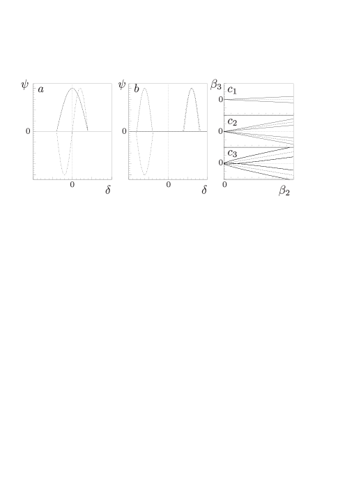
Figure 3: The lowest even and odd parity wavefunctions in a separable model with $\delta$ restricted to a small interval around 0 (part $a$) or around $\pm\delta_{0}$ (part $b$). The part $c$ shows the corresponding allowed regions in the $\beta_{2}-\beta_{3}$ plane ($c_{1}$ and $c_{2}$, respectively) and the region corresponding to one standard deviation for the localized wavefunctions in the schematic model discussed in the text ($c_{3}$).

How can we proceed? A possible way out is to assume a potential, symmetric in $\delta$, and approaching the harmonic behaviour around $\delta\approx\pm\delta_{0}$. In this case, the equation is no longer separable in the entire field. For large values of $\beta$, one still finds localized solutions, with a $\beta$ dependent extension around the average value ($\pm\delta_{0}$): for a fixed value of $\beta$, the variance of $\delta$ would have the form $D^{2}(\delta)=C/\beta$. As $\beta\rightarrow 0$, the two localized solutions start to overlap (Fig. 3 $c_{3}$), and this would remove the degeneracy of even and odd combinations, as long as the wavefunctions in $\beta$ have a non-negligible value in the region where the overlap is significant. At moderately large values of $J$, the significant values of $\psi(\beta)$ are pushed out of this region by the centrifugal-like term of Eq. 35, and the staggering will disappear.

Although this approximation is certainly insufficient just in the region of overlap, we think it can give a qualitative explanation of the behaviour of the negative–parity band (not far from the point of view of Jolos and von Brentano [17]) and, perhaps, give some indication for future developments.

References

- [1] P.G. Bizzeti, and A.M. Bizzeti-Sona (2004) Phys. Rev. C 70 064319.
- [2] L. Bargioni et al. (1996) Phys. Rev. C 51 R1057.
- [3] Zs. Podolyák et al. (2000) Europ.Phys. J. A 8 147.
- [4] F. Iachello (2000) Phys. Rev. Lett. 85 3580.
- [5] F. Iachello (2001) Phys. Rev. Lett. 87 052502.
- [6] F. Iachello (2003) Phys. Rev. Lett. 91 132502.
- [7] D. Bonatsos et al. (2004) Phys. Lett. B 588 172
- [8] R.F. Casten and N.V. Zamfir, Phys. Rev. Lett. 87 052503.
- [9] P.G. Bizzeti, and A.M. Bizzeti-Sona (2002) Phys. Rev. C 66 031301.
- [10] P.G. Bizzeti, and A.M. Bizzeti-Sona (2004) Eur. Phys. J. A 20 179.
- [11] P.G. Bizzeti (2003) in Symmetries in Nuclear Structure (ed. A. Vitturi and R. Casten; World Scientific, Singapore) p. 262.
- [12] C.Hutter et al (2003) Phys. Rev. C 67 054315.
- [13] A.I. Georgieva, H.G. Ganev, J.P. Draayer (2005); H.G. Ganev, A.I. Georgieva, J.P. Draayer (2005); V.P. Garistov, A.A. Solnyshkin, A.I. Georgieva, V.V. Burov, H.G. Ganev (2005) These Proceedings.
- [14] C.E. Alonso et al. (1995) Nucl. Phys. A 586 100; A.A. Raduta and D. Ionescu (2003) Phys. Rev. C 67 044312; N.V. Zamfir and D. Kunezov (2003) Phys. Rev. C 67 014305; and references therein.
- [15] W. Donner and W. Greiner (1966) Z. Phys. 197 440.
- [16] P.A. Butler and Nazarewicz (1996) Rev. Mod. Phys. 68 349, and references therein.
- [17] R.V. Jolos and P. von Brentano (1999) Phys. Rev. C 60 064317.
- [18] N. Minkov et al. (2001) Phys. Rev. C 63 044305; N. Minkov et al. (2004) Proc. of the 23th Int. Workshop on Nuclear Theory (ed. S. Dimitrova, Sofia) p. 203.
- [19] C. Wexler and G.G. Dussel (1999) Phys. Rev. C 60 014305.
- [20] W. Pauli (1933) in Handbuch der Physik (Springer, Berlin) Vol. XXIV/I.
- [21] N. Minkov, These Proceedings.
- [22] J. Eisenberg and W. Greiner (1987) Nuclear Models (North Holland, Amsterdam).
- [23] See Section 6.1 of ref. [22].
- [24] L.Fortunato (2005) These Proceedings.
- [25] W. Nazarewicz and P. Olanders (1985) Nucl. Phys. A 441 420.