Two-particle interferometry for non-central heavy-ion collisions

Abstract

In non-central heavy ion collisions, identical two particle Hanbury-Brown/Twiss (HBT) correlations $C({\bf K},{\bf q})$ depend on the azimuthal direction of the pair momentum ${\bf K}$. We investigate the consequences for a harmonic analysis of the corresponding HBT radius parameters $R_{ij}^{2}$. Our discussion includes both, a model-independent analysis of these parameters in the Gaussian approximation, and the study of a class of hydrodynamical models which mimic essential geometrical and dynamical properties of peripheral heavy ion collisions. Also, we discuss the additional geometrical and dynamical information contained in the harmonic coefficients of $R_{ij}^{2}$. The leading contribution of their first and second harmonics are found to satisfy simple constraints. This allows for a minimal, azimuthally sensitive parametrization of all first and second harmonic coefficients in terms of only two additional fit parameters. We determine to what extent these parameters can be extracted from experimental data despite finite multiplicity fluctuations and the resulting uncertainty in the reconstruction of the reaction plane.

I Introduction

The goal of the current and future experimental heavy ion programs at CERN and BNL is to test the equilibration properties of hadronic matter at energy densities where quarks and gluons are the relevant physical degrees of freedom. Anisotropic (directed) transverse flow is an important observable for this program, since both hydrodynamic and thermodynamic behaviour is based on equilibration processes between local degrees of freedom. Hydrodynamical flow effects result from pressure gradients which due to compression of the hadronic matter build up during the collision process. Their strength depends on the equation of state of the hot matter and provides insight into the collision dynamics. Moreover, hadronic observables mainly test the final collision stage and a back extrapolation is needed to extract from them information about the hot and dense earlier stages. For this to work, collective and random (’thermal’) motion in the collision region have to be distinguished properly. Hence, concepts of different types of collective flow play a central role in understanding the dynamics of heavy ion collisions.

Directed anisotropic flow was observed in both AGS [1, 2] and SPS [3, 4] experiments, as well as at lower BEVALAC/SIS energies [5]. Directivity[3, 4], 2- and 3-dimensional sphericity [6, 7, 8], or the so-called deformation parameter $R_{p}$ [5] are typical variables used in its characterization. With minor differences, all of them are sensitive to azimuthal anisotropies in the triple-differential particle distributions. The most complete experimentally feasible parametrization is obtained in a Fourier expansion in the azimuthal angle for different values of rapidity and transverse momentum, [9, 1, 2, 10]

$$E{dN\over d^{3}p} = {d^{3}N\over p_{t}\,dp_{t}\,dy\,d\phi}=\int d^{4}xS(x,p)$$ (1)

$$= \textstyle{1\over 2\pi}{d^{2}N\over p_{t}\,dp_{t}\,dy}[1+2\sum_{n=1}^{\infty}v_{n}\cos n(\phi-\psi_{R}^{(n)})]\,.$$ (2)

Here, the azimuthal angles $\psi_{R}^{(n)}$ allow for the determination of the reaction plane and the harmonic coefficients $v_{n}$ characterize the size of the total vector sum of transverse momenta ($n=1$), the approximate elliptic shape of the azimuthal distribution ($n=2$) and higher order triangle-type ($n=3$), rectangle-type ($n=4$) etc. deformations.

In Eq. (2), we have expressed the one-particle distribution in terms of the emission function $S(x,p)$ which specifies the collision region at freeze-out. $S(x,p)$ is a Wigner distribution and denotes the phase space probability that a particle of four momentum $p$ is emitted from a space-time point $x$ in the collision region. Features of collective dynamics as e.g. directed flow are encoded in the source function $S(x,p)$ as $x$-$p$ position-momentum correlations. Observables extracted from the one-particle distributions (2) are not sensitive to the space-time characterisitics (and a fortiori to $x$-$p$ correlations) of the source. The question arises to what extent observables which are sensitive to $x$-$p$ correlations can support and refine the picture obtained via the analysis of (2). This motivates an azimuthally sensitive Hanbury-Brown Twiss analysis of 2-particle correlation functions, which is the main focus of the present work.

Identical two-particle correlations $C({\bf K},{\bf q})$, here written in terms of the average $K=\textstyle{1\over 2}(p_{1}+p_{2})$ and relative $q=p_{1}-p_{2}$ pair momentum, are the only known observables sensitive to space-time characteristics of the source. Their space-time interpretation is based on the result [11, 12, 13, 14]

$$C({\bf K},{\bf q}) = 1+|\langle e^{i{\bf q}{\cdot}({\bf x}-\vec{\beta}t)}\rangle|\,,$$ (3)

$$\langle f(x)\rangle = {\int d^{4}xf(x)S(x,K)\over\int d^{4}xS(x,K)}\,,$$ (4)

where we have used the on-shell condition $q\cdot K=0$ to substitute the temporal component $q^{0}$ in the 4-dimensional Fourier transform, $\vec{\beta}={\bf K}/K_{0}$. According to (4), determining $K$-dependent geometrical and dynamical source infomation reduces to a Fourier inversion problem (which due to the on-shell constraint however does not have a unique solution). In the standard analysis of (4), one assumes an azimuthally symmetric collision and characterizes $C({\bf K},{\bf q})$ with four Gaussian Hanbury-Brown/Twiss HBT radius parameters which depend on $|{\bf K}_{\perp}|$ and the longitudinal pair rapidity $Y$ only [16]. In contrast, the anisotropic case requires six HBT radius parameters $R_{ij}$ which in addition depend on the azimuthal angle $\Phi$ of ${\bf K}_{\perp}$ [15]. Previous discussions of the azimuthal dependence of $C({\bf K},{\bf q})$ were based on event generator studies [17, 18] for finite impact parameter collisions, or exploited the Lorentz invariance of the correlator to derive azimuthally dependent HBT radius parameters [19]. The present work is complementary to these and starts in analogy to (2) from expanding the angular dependence of $C({\bf K},{\bf q})$ in a harmonic series,

$$C({\bf K},{\bf q}) = 1+\exp{\left({\sum_{ij}R_{ij}^{2}q_{i}q_{j}}\right)}\,,$$ (5)

$$R_{ij}^{2}(K_{\perp},\Phi,Y) = R_{ij,0}^{2}(K_{\perp},Y)$$ (6)

$$+ 2\sum_{n=1}^{\infty}{R^{c}_{ij,n}}^{2}(K_{\perp},Y)\cos n\Phi$$ (7)

$$+ 2\sum_{n=1}^{\infty}{R^{s}_{ij,n}}^{2}(K_{\perp},Y)\sin n\Phi\,.$$ (8)

Here, the components $i$,$j$ are given in the “out-side-long” osl-system where the relative pair momentum has a transverse out component $q_{o}$ parallel to the pair momentum ${\bf K}_{\perp}$, a longitudinal long component $q_{l}$ along the beam and a remaining side component. To discuss the azimuthal $\Phi$-dependence of the two-particle correlator (8), we frequently use an impact-parameter fixed system. In this system, the direction of the impact parameter $\vec{b}$ specifies the $x$-axis, the $z$-axis is along the beam and the $y$-axis is perpendicular to the reaction plane spanned by $x$ and $z$. Accordingly, the total angular momentum $\vec{L}$ of the system, with

$$L_{i}=\epsilon_{ijk}\langle\!\langle x_{j}\,p_{k}\,\rangle\!\rangle=\epsilon_{ijk}\int{d^{3}p\over E}\int d^{4}x\,x_{j}\,p_{k}\,S(x,p)\,,$$ (9)

points along the $y$ direction.

One central theme of the following is to determine those harmonic coefficients ${R_{ij,n}^{c}}^{2}$, ${R_{ij,n}^{s}}^{2}$, whose contributions are not negligible. We shall find that there are very few independent ones. This makes a comparisons with experimental data feasible. Also, we aim at understanding which geometrical and dynamical information about the particle emitting source is contained in the harmonic coefficients. In section II, we attack both problems by deriving model-independent expressions for the HBT radius parameters. These allow for the calculation of HBT radii from $\Phi$-dependent space-time variances $\langle x_{\mu}x_{\nu}\rangle$ of arbitrary model emission functions $S(x,K)$. Investigating the $\Phi$-dependence of $\langle x_{\mu}x_{\nu}\rangle$ leads then to relations between the harmonic coefficients in (8). In the more detailed model-independent discussion in section III and the subsequent model study in section IV, we restrict our investigation to mid-rapidity and to symmetric collision systems. Due to the reflection symmetry with respect to the $y$-$z$-plane, all odd harmonic coefficients vanish in this case, and this considerably simplifies the discussion. In section V, we extend this analysis to the fragmentation regions. Again, we derive simple relations between the non-vanishing first harmonic coefficients, and we illustrate our findings quantitatively in a subsequent model study. The discussion in sections II-V implicitly assumes that the orientation $\psi_{R}$ of the reaction plane is known. It hence neglects finite multiplicity fluctuations which introduce in practice a significant uncertainty in determining $\psi_{R}$. In section VI we investigate to what extent information about the anisotropy of the correlator $C({\bf K},{\bf q})$ can be obtained despite these statistical constraints. The main results are then summarized in the Conclusion.

II Azimuthal Dependence of Cartesian HBT Radius Parameters

Here, we derive model-independent expressions for the Cartesian HBT radius parameters (8) in terms of space-time variances [16, 15] of the emission function $S(x,K)$. These radius parameters depend in general on the azimuthal orientation of the pair momentum ${\bf K}$ which we define with respect to the direction of the impact parameter $\vec{b}$,

$$\Phi=\angle(\vec{\bf K}_{\perp},\vec{b})\,.$$ (10)

They can be calculated as second derivatives of the correlator $C({\bf K},{\bf q})$ with respect to the relative momentum components $i,j=o,s,l$ in the osl-system. In what follows, we consider the emission function $S(x,K)$ to be given in the impact parameter fixed coordinate system. Then, to express the HBT radii in terms of space-time variances, one has to rotate the coordinate system by the angle $\Phi$,

$$({\cal D}_{\Phi}\vec{\beta})=\left(\begin{array}[]{c}\beta_{\perp}\\ 0\\ \beta_{l}\end{array}\right)\,,{\cal D}_{\Phi}\vec{\tilde{x}}=\left(\begin{array}[]{c}\tilde{x}\cos\Phi+\tilde{y}\sin\Phi\\ -\tilde{x}\sin\Phi+\tilde{y}\cos\Phi\\ \tilde{z}\end{array}\right)\,,$$ (18)

$$R_{ij}^{2}({\bf K})=-\left.{\partial^{2}C({\bf q},{\bf K})\over\partial q_{i}\,\partial q_{j}}\right|_{{\bf q}=0}\,$$ (19)

$$=\langle[({\cal D}_{\Phi}\tilde{x})_{i}-({\cal D}_{\Phi}\beta)_{i}\tilde{t}][({\cal D}_{\Phi}\tilde{x})_{j}-({\cal D}_{\Phi}\beta)_{j}\tilde{t}]\rangle\,.$$ (20)

Here, $\tilde{x}_{\mu}=x_{\mu}-\langle x_{\mu}\rangle$, and all coordinates $x$, $y$ and $z$ are given in the impact-parameter fixed system. The space-time variances specify the curvature of the correlator at ${\bf q}=0$ and coincide with the experimentally determined half widths of $C({\bf K},{\bf q})$ for Gaussian shapes only [20, 21]. Deviations from a Gaussian can be characterized by more refined methods [21]. The present investigation is restricted to correlators of sufficiently Gaussian shape and makes no attempt to quantify (possibly $\Phi$-dependent) non-Gaussian deviations. In the analysis of azimuthally symmetric HBT correlation radii, this Gaussian approximation has led to a qualitative and quantitative understanding of the $K_{\perp}$-dependence of correlation functions [15]. This motivates us to adopt the same starting point for an azimuthally sensitive analysis. The six $\Phi$-dependent HBT radius parameters (20) read

$$R_{s}^{2}(K_{\perp},\Phi,Y)=\langle\tilde{x}^{2}\rangle\sin^{2}\Phi+\langle\tilde{y}^{2}\rangle\cos^{2}\Phi-\langle\tilde{x}\tilde{y}\rangle\sin 2\Phi\,,$$ (21)

$$R_{o}^{2}(K_{\perp},\Phi,Y)=\langle\tilde{x}^{2}\rangle\cos^{2}\Phi+\langle\tilde{y}^{2}\rangle\sin^{2}\Phi+\beta_{\perp}^{2}\langle\tilde{t}^{2}\rangle$$ (22)

$$\qquad\qquad-2\beta_{\perp}\langle\tilde{t}\tilde{x}\rangle\cos\Phi-2\beta_{\perp}\langle\tilde{t}\tilde{y}\rangle\sin\Phi+\langle\tilde{x}\tilde{y}\rangle\sin 2\Phi\,,$$ (23)

$$R_{os}^{2}(K_{\perp},\Phi,Y)=\langle\tilde{x}\tilde{y}\rangle\cos 2\Phi+\textstyle{1\over 2}\sin 2\Phi(\langle\tilde{y}^{2}\rangle-\langle\tilde{x}^{2}\rangle)$$ (24)

$$\qquad\qquad+\beta_{\perp}\langle\tilde{t}\tilde{x}\rangle\sin\Phi-\beta_{\perp}\langle\tilde{t}\tilde{y}\rangle\cos\Phi\,,$$ (25)

$$R_{l}^{2}(K_{\perp},\Phi,Y)=\langle(\tilde{z}-\beta_{l}\tilde{t})^{2}\rangle\,,$$ (26)

$$R_{ol}^{2}(K_{\perp},\Phi,Y)=\langle(\tilde{z}-\beta_{l}\tilde{t})(\tilde{x}\cos\Phi+\tilde{y}\sin\Phi-\beta_{\perp}\tilde{t})\rangle\,,$$ (27)

$$R_{sl}^{2}(K_{\perp},\Phi,Y)=\langle(\tilde{z}-\beta_{l}\tilde{t})(\tilde{y}\cos\Phi-\tilde{x}\sin\Phi)\rangle\,.$$ (28)

These equations separate the explicit $\Phi$-dependence of the HBT-radii (which is a consequence of the changing direction of the pair momentum ${\bf K}$ with respect to the reaction plane) from the implicit $\Phi$-dependence of the spatio-temporal widths $\langle\tilde{x}_{\mu}\tilde{x}_{\nu}\rangle$ (which reflects a $\Phi$-dependent change of the shape of the effective emission region). In general, both implicit and explicit $\Phi$-dependence will show up in the harmonic coefficients

$${R_{ij,m}^{c}}^{2} = \textstyle{1\over 2\pi}\int_{-\pi}^{\pi}R_{ij}^{2}\,\cos(m\Phi)\,d\Phi\,,$$ (30)

$${R_{ij,m}^{s}}^{2} = \textstyle{1\over 2\pi}\int_{-\pi}^{\pi}R_{ij}^{2}\,\sin(m\Phi)\,d\Phi\,,$$ (31)

which determine the complete Gaussian parametrization (8).

The following discussion of the $\Phi$-dependent HBT radius parameters (28) is focussed mainly on the transverse parameters $R_{s}^{2}$, $R_{o}^{2}$, $R_{os}^{2}$. Their harmonic coefficients depend on the $\Phi$-dependence of the transverse spatial widths

$$T_{ij}^{\perp}=\langle\tilde{x}_{i}\tilde{x}_{j}\rangle\,,$$ (32)

$i$, $j$ being components in the transverse plane. Any $\Phi$-dependence of $T^{\perp}$ is a consequence of non-trivial $x$-$\Phi$ correlations and a fortiori of position-momentum correlations in the source. To illustrate this point, we have sketched in Fig. 1 two simplified scenarios. If there are no $x$-$\Phi$-correlations, then the transverse shape of the effective emission region is $\Phi$-independent and reflects the global geometry of the collision region. For non-trivial $x$-$\Phi$ correlations, this simple relation between the emission region and the global geometry breaks down. In sections III and V, we find observable combinations of first and second harmonic coefficients which are sensitive to this difference. More generally, we classify the possible $\Phi$-dependences of (32) and discuss their implications for the harmonic analysis of HBT radius parameters.

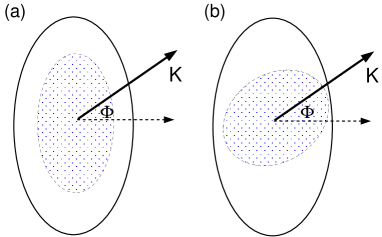
FIG. 1.: Schematic picture of a transverse cut through the collision region. Shaded is the effective emission region contributing to the correlator for pair momentum ${K}$. Two different scenarios are shown: in (a) the anisotropy is determined by the global geometry of the collision, in (b) it is significantly influenced by the collective dynamics of the source. Both scenarios can be distinguished experimentally, see the text.

We conclude this section by shortly commenting on the $\Phi$-dependence of $R_{l}^{2}$, $R_{ol}^{2}$ and $R_{sl}^{2}$. The longitudinal radius parameter $R_{l}^{2}$ shows no explicit $\Phi$-dependence and coincides formally with the expression for the azimuthally symmetric case [16]. The radii $R_{ol}^{2}$ and $R_{sl}^{2}$ contain explicit $\Phi$-dependent terms proportional to $\langle\tilde{t}\tilde{x}\rangle$ or $\langle\tilde{t}\tilde{y}\rangle$. These characterize asymmetries of the particle emission probability around the point of highest emissivity and they vanish for models with Gaussian emission functions $S(x,k)$. In the light of this, we consider in what follows all harmonic coefficients $m\geq 1$ of the HBT radii $R_{l}^{2}$, $R_{ol}^{2}$, $R_{sl}^{2}$ to be negligible,

$${R_{l,m}^{c}}^{2} = {R_{l,m}^{s}}^{2}\approx 0\,,$$ (34)

$${R_{ol,m}^{c}}^{2} = {R_{ol,m}^{s}}^{2}\approx 0\,,$$ (35)

$${R_{sl,m}^{c}}^{2} = {R_{sl,m}^{s}}^{2}\approx 0\,.$$ (36)

This is a reasonable but model-dependent assumption. For all models studied below, we have checked (1) numerically, see section IV B.

III Azimuthal analysis of the mid-rapidity region

In this section, we discuss the azimuthal analysis of 1- and 2-particle spectra for symmetric collision systems like Pb-Pb or Au-Au at mid-rapidity. The important simplification at mid-rapidity is that all observables are invariant under $\Phi\to\Phi+\pi$, a $180^{o}$-rotation in the transverse plane. All odd harmonic coefficients vanish. This is different for the fragmentation region or for non-symmetric collision systems where the only remaining symmetry is that with respect to the reaction plane. The arising complications are discussed in section V. Here, we first discuss a scenario, for which the space-time variances (32) do not depend on the azimuthal direction of ${\bf K}_{\perp}$. Then, we turn to the discussion of an arbitrary $\Phi$-dependence of $T^{\perp}$.

A The elliptic approximation

We start by considering an elliptic approximation of the transverse spatial widths $T_{ij}^{\perp}$. This toy example will be useful in the sequel for comparisons with the general case. It provides a simple picture for the consequences of a purely geometrical scenario, and it can account for some of the main features of the harmonic coefficients, calculated in the model study in section IV.

In the elliptic approximation, we characterize the tensor $T^{\perp}$ by its principal axes (eigenvectors) $\vec{g}_{1}$, $\vec{g}_{2}$, and the corresponding eigenvalues $g_{1}$ and $g_{2}$. If the orientation of the reaction plane and $\vec{g}_{1}$ differs by an angle $\varphi$, then $T_{ij}^{\perp}$ takes a simple form in the impact-parameter fixed system,

$$T^{\perp} = \bar{g}\left(\begin{array}[]{cc}1+\alpha_{T}\cos 2\varphi&-\alpha_{T}\sin 2\varphi\\ -\alpha_{T}\sin 2\varphi&1-\alpha_{T}\cos 2\varphi\end{array}\right)\,,$$ (40)

$$\bar{g} = \textstyle{1\over 2}(g_{1}+g_{2})\,,\,\qquad\alpha_{T}={{g_{1}-g_{2}}\over{g_{1}+g_{2}}}\,.$$ (41)

This is somewhat analogous to the expression of the transverse sphericity tensor in [7, 8]. It provides a convenient parametrization of the three independent expectation values $\langle\tilde{x}_{i}\tilde{x}_{j}\rangle$ in terms of the average size $\bar{g}$ of the homogeneity region, its transverse spatial anisotropy $\alpha_{T}$ and the orientation $\varphi$ of its principal axis $\vec{g}_{1}$ with respect to the reaction plane. In case of an azimuthally symmetric collision with vanishing impact parameter, $\varphi=0$, the cross term vanishes, $\langle\tilde{x}_{s}\tilde{x}_{o}\rangle=0$, and the spatial asymmetry $\alpha_{T}$ in (40), (41) describes the difference between the spatial widths in the out- and side-directions. In terms of these parameters, the ‘transverse’ HBT radii $R_{o}$, $R_{s}$ and $R_{os}$ read

$$R_{s}^{2}(K_{\perp},\Phi,Y) = \bar{g}{\left({1-\alpha_{T}\cos 2(\varphi+\Phi)}\right)}\,,$$ (43)

$$R_{o}^{2}(K_{\perp},\Phi,Y) = \bar{g}{\left({1+\alpha_{T}\cos 2(\varphi+\Phi)}\right)}$$ (45)

$$+\beta_{\perp}^{2}\langle\tilde{t}^{2}\rangle+C_{o}\,,$$

$$R_{os}^{2}(K_{\perp},\Phi,Y) = -\bar{g}\alpha_{T}\sin 2(\varphi+\Phi)+C_{os}\,,$$ (46)

$$C_{o} = -2\beta_{\perp}\langle\tilde{t}\tilde{x}\rangle\cos\Phi-2\beta_{\perp}\langle\tilde{t}\tilde{y}\rangle\sin\Phi\,,$$ (47)

$$C_{os} = +\beta_{\perp}\langle\tilde{t}\tilde{x}\rangle\sin\Phi-\beta_{\perp}\langle\tilde{t}\tilde{y}\rangle\cos\Phi\,.$$ (48)

The two correction terms $C_{o}$, $C_{os}$ contain widths $\langle\tilde{t}\tilde{x}_{i}\rangle$ which are linear in $\tilde{t}$ and measure asymmetries of the source around the point of highest emissivity. At mid-rapidity, all observables are invariant under $\Phi\to\Phi+\pi$, and $\langle\tilde{x}\tilde{t}\rangle(\Phi+\pi)=-\langle\tilde{x}\tilde{t}\rangle(\Phi)$. The correction terms hence do not contribute to the first harmonic coefficients ${R_{ij,1}}^{2}$, but to the second ones. Moreover, they vanish for emission functions $S(x,K)$ which are Gaussian in the spatial components. Their contribution to $R_{o}^{2}$, $R_{os}^{2}$ is neglected in the remainder of this section, and the validity of this approximation is checked in the numerical model study of section IV.

The main assumption of the elliptic approximation which we avoid in section III B, is that the parameters $\bar{g}$ and $\alpha_{T}$ do not depend on the azimuthal orientation of ${K}_{\perp}$. The homogeneity region is determined entirely by the geometry, cf. Fig. 1a. The eigenvectors $\vec{g}_{1}$, $\vec{g}_{2}$ lie parallel and orthogonal to the reaction plane and the angle $\varphi$ should vanish; it hence accounts only for the statistical uncertainty in determining the reaction plane, see section VI. Comparing the expressions (III A) with the Fourier expansion (8) of the HBT radius parameters, we find for $\varphi=0$

$${R_{o,0}}^{2} = \bar{g}+\beta_{\perp}^{2}\langle\tilde{t}^{2}\rangle\,,\qquad{R_{s,0}}^{2}=\bar{g}\,,$$ (50)

$${R_{o,2}^{c}}^{2} = -{R_{s,2}^{c}}^{2}=-{R_{os,2}^{s}}^{2}=\textstyle{1\over 2}\alpha_{T}\bar{g}\,.$$ (51)

The other second and higher order Fourier coefficients vanish. According to (III A), the ansatz (8) for the correlator contains redundant information. In the present case, neither the shape of $T^{\perp}$ nor the size of the homogeneity region depend on $\Phi$ while the anisotropy terms of the HBT radius parameters are sufficiently many to encode for such a non-trivial $\Phi$-dependence.

B The general case

To discuss an arbitrary $\Phi$-dependence of the transverse spatial widths, we start from a complete Fourier expansion of $T^{\perp}_{ij}=\langle\tilde{x}_{i}\tilde{x}_{j}\rangle$, respectively of its linear combinations

$$A = \textstyle{{\langle\tilde{x}^{2}\rangle+\langle\tilde{y}^{2}\rangle}\over 2}=\sum_{n=0}^{\infty}\left(A_{n}\cos n\Phi+A^{\prime}_{n}\sin n\Phi\right)\,,$$ (52)

$$B = \textstyle{{\langle\tilde{x}^{2}\rangle-\langle\tilde{y}^{2}\rangle}\over 2}=\sum_{n=0}^{\infty}\left(B_{n}\cos n\Phi+B^{\prime}_{n}\sin n\Phi\right)\,,$$ (53)

$$C = \langle\tilde{x}\tilde{y}\rangle=\sum_{n=0}^{\infty}\left(C^{\prime}_{n}\cos n\Phi+C_{n}\sin n\Phi\right)\,.$$ (54)

Here, the coefficients $A_{n}$, $A^{\prime}_{n}$, etc. are functions of the longitudinal pair rapidity $Y$ and the transverse pair momentum $|{\bf K}_{\perp}|$, only. The symmetry of the collision region with respect to the reaction plane implies that the terms $\langle\tilde{x}^{2}\rangle$, $\langle\tilde{y}^{2}\rangle$ are invariant under $\Phi\to-\Phi$, while the term $\langle\tilde{x}\tilde{y}\rangle$ changes its sign. Calculating the coefficients in (54) via Fourier transform, it is easy to check that the primed ones vanish,

$$A^{\prime}_{n}=B^{\prime}_{n}=C^{\prime}_{n}=0\,.$$ (55)

The general $\Phi$-dependent HBT radius parameters (28) read

$$R_{s}^{2} = A-B\cos 2\Phi-C\sin 2\Phi\,,$$ (56)

$$R_{o}^{2} = A+B\cos 2\Phi+C\sin 2\Phi+\beta_{\perp}^{2}\,\langle\tilde{t}^{2}\rangle\,,$$ (57)

$$R_{os}^{2} = -B\sin 2\Phi+C\cos 2\Phi\,,$$ (58)

where we have dropped the small correction terms $C_{o}$, $C_{os}$. From these HBT radius parameters (58) one can calculate the harmonic coefficients (II). Especially, we obtain the zeroth harmonics

$$R_{s,0}^{2} = A_{0}-\textstyle{1\over 2}B_{2}-\textstyle{1\over 2}C_{2}\,,$$ (59)

$$R_{o,0}^{2} = A_{0}+\textstyle{1\over 2}B_{2}+\textstyle{1\over 2}C_{2}+\beta_{\perp}^{2}\,\langle\tilde{t}^{2}\rangle\,,$$ (60)

$$R_{os,0}^{2} = 0\,,$$ (61)

and the second harmonic coefficients

$${R_{s,2}^{c}}^{2} = -\textstyle{1\over 2}B_{0}+\textstyle{1\over 2}A_{2}-\textstyle{1\over 4}B_{4}-\textstyle{1\over 4}C_{4}\,,$$ (62)

$${R_{o,2}^{c}}^{2} = \textstyle{1\over 2}B_{0}+\textstyle{1\over 2}A_{2}+\textstyle{1\over 4}B_{4}+\textstyle{1\over 4}C_{4}\,,$$ (63)

$${R_{os,2}^{s}}^{2} = -\textstyle{1\over 2}B_{0}+\textstyle{1\over 4}B_{4}+\textstyle{1\over 4}C_{4}\,,$$ (64)

$${R_{s,2}^{s}}^{2} = {R_{o,2}^{s}}^{2}={R_{os,2}^{c}}^{2}=0\,.$$ (65)

For the case of $\Phi$-independent spatial widths $T^{\perp}$, only the terms with index $0$ survive on the right hand side, and (65) coincides with (51) for $A_{0}=\bar{g}$ and $B_{0}=\alpha_{T}\bar{g}$. If deviations from (51) are observed, this is an unambiguous sign for source gradients leading to a $\Phi$-dependence of $T_{ij}^{\perp}$. From the absence of such deviations, however, one cannot conclude that there are no source gradients. In the following model study we shall find that even in the presence of sizeable source gradients, such deviations can be small. Then, the use of equations (51) resides in reducing the number of fit parameters in an azimuthal HBT-analysis, see section VI.

Let us finally anticipate that for the models studied below, the fourth harmonic coefficients $A$, $B$ and $C$ are negligible. It follows from (65) that then the deviations of (51) are essentially determined by the term $\textstyle{1\over 2}A_{2}$ only, i.e.,

$${R_{o,2}^{c}}^{2}+2\,{R_{os,2}^{s}}^{2}\approx{R_{s,2}^{c}}^{2}\,.$$ (66)

IV A model calculation

We introduce now a simple hydrodynamical model for the emission function of a heavy ion collision which includes anisotropy effects. For this model, we calculate both the one- and two-particle spectra, illustrating the main points of the above model-independent discussion.

In the central rapidity region of a peripheral collisions, the initial distribution of the highly excited nuclear matter is given by the intersection of the nuclear spheres. The largest pressure gradient developping from such initial conditions is expected to be aligned with the impact parameter $\vec{b}$, cf.  [7, 18]. To mimic this scenario, we consider the class of model emission functions

$$S(x,K)=\tau_{0}m_{\perp}\cosh(\eta-y)\,\exp\left(\textstyle{-K^{\mu}u_{\mu}(x)\over T}\right)\,H(x)\,,$$ (67)

whose azimuthally symmetric versions have been discussed extensively in the literature. For a review, cf. [15]. These models assume the emission of particles from a thermalized system with collective four-velocity $u_{\mu}$, confined in a space-time volume determined by $H(x)$. The factor $P\cdot n(x)=\tau_{0}m_{\perp}\cosh(\eta-y)$ specifies a simple hyperbolic freeze-out hypersurface. We introduce an azimuthal anisotropy in the source both via an elliptic shape of the geometrical emission region,

$$H(x)=\exp\left[-{(\tau-\tau_{0})^{2}\over 2(\Delta\tau)^{2}}-{{(\eta-\eta_{0})}^{2}\over 2(\Delta\eta)^{2}}-{x^{2}\over 2\rho_{x}^{2}}-{y^{2}\over 2\rho_{y}^{2}}\right],$$ (68)

and via an azimuthally asymmetric flow pattern $u_{\mu}(x)$ which is properly normalized, $u_{\mu}u^{\mu}=1$,

$$u_{\mu}(x) = (u_{l}\cosh\eta,u_{x},u_{y},u_{l}\sinh\eta)\,,$$ (69)

$$u_{x} = \textstyle{x\over\lambda_{x}}\,,\,\,u_{y}=\textstyle{y\over\lambda_{y}}\,,\,\,u_{l}=\sqrt{1+u_{x}^{2}+u_{y}^{2}}\,.$$ (70)

In the longitudinal direction, we choose a boost invariant flow pattern satisfying Bjorken scaling [22], i.e., the main energy flow is along the beam axis. Instead of the variables $\rho_{x}$, $\rho_{y}$, $\lambda_{x}$, $\lambda_{y}$, we use in what follows the transverse size $R$ and its spatial anisotropy $\epsilon_{s}$, as well as the transverse flow strength $\eta_{f}$ and the corresponding flow anisotropy $\epsilon_{f}$,

$$\rho_{x} = R\sqrt{1-\epsilon_{s}}\,,\qquad\rho_{y}=R\sqrt{1+\epsilon_{s}}\,,$$ (72)

$$u_{x} = \eta_{f}\sqrt{1+\epsilon_{f}}\textstyle{x\over R}\,,\qquad u_{y}=\eta_{f}\sqrt{1-\epsilon_{f}}\textstyle{y\over R}\,.$$ (73)

We have chosen the principal axes of the transverse space-time distribution aligned with those of the azimuthal momentum distribution, since the dynamical evolution of the collision region cannot break the reflection symmetry of the system with respect to the reaction plane. The spatial anisotropy $\epsilon_{s}$ takes values in the range $-1<\epsilon_{s}<1$, i.e., for $\epsilon>0$, the collision region is longer in the direction perpendicular to $\vec{b}$, $\rho_{x}<\rho_{y}$. For the flow anisotropy $\epsilon_{f}$, we allow for $-1<\epsilon_{f}<1$; the major flow component lies in the reaction plane if $\epsilon_{f}$ is positive. All numerical calculations are done for the input parameters $T=150$ MeV, $m=m_{\pi}=139$ MeV, $\tau_{0}=5$ fm/c, $\Delta\tau=1$ fm/c, $\Delta\eta=1.22$ and $R=5$ fm. We study the dependence of the 1- and 2-particle spectra on the size of the transverse flow, and the spatial $\epsilon_{s}$ and dynamical $\epsilon_{f}$ anisotropies.

A Harmonic analysis of azimuthal particle distributions

The harmonic coefficients $v_{n}$ of the triple-differential one-particle spectrum (2) are given in terms of the Fourier transforms

$$\left(\begin{array}[]{c}a_{n}\\ b_{n}\end{array}\right)={{\int_{0}^{2\pi}E\textstyle{dN\over d^{3}p}\left({\begin{array}[]{c}\cos(n\phi)\\ \sin(n\phi)\end{array}}\right)\,d\phi}\over{\int_{0}^{2\pi}E\textstyle{dN\over d^{3}p}d\phi}}\,,$$ (74)

$$a_{n}=v_{n}\,\cos(n\psi_{R}^{(n)})\,,\qquad b_{n}=v_{n}\,\sin(n\psi_{R}^{(n)})\,.$$ (75)

The zeroth harmonic $v_{0}$ denotes the azimuthally averaged double differential particle distribution, all other anisotropy parameters $v_{n}$ characterize azimuthal asymmetries in the momentum distribution.

In the absence of transverse flow, $\eta_{f}=0$, the model (67) does not contain source gradients in the transverse plane. Irrespective of whether the transverse geometry of the source is radially symmetric ($\epsilon_{s}=0$) or not, particle emission is isotropic in the transverse plane. All harmonic coefficients $v_{n}$, $n\geq 1$, vanish.

In the presence of transverse flow, the reflection symmetry of the emission function (67) in the direction of the impact parameter implies a $\phi\to\phi+\pi$ symmetry of the particle spectra. All odd harmonic coefficients $v_{n}$ vanish. The lowest non-vanishing anisotropy parameter is $v_{2}$. This parameter is positive if the spectrum $d^{3}N/(p_{t}\,dp_{t}\,dy\,d\phi)$ shows a maximum in the reaction plane, it is negative for the opposite case. Higher fourth (6th, etc.) harmonic coefficients are found to be much smaller. They are not discussed further.

The transverse pair momentum dependence of the corresponding normalized quantity $v_{2}/v_{0}$ is depicted in Fig. 2 for different physical scenarios. Irrespective of the model parameters $\eta_{f}$, $\epsilon_{s}$ and $\epsilon_{f}$, the coefficient $v_{2}/v_{0}$ vanishes at $K_{\perp}=0$ and is growing monotonously with the transverse pair momentum. This is a direct consequence of the Lorentz-invariant Boltzmann term in (67) which encodes the assumption of local thermal equilibrium,

$$K^{\mu}u_{\mu}=\textstyle{{m_{\perp}}\over T}\cosh(\eta-Y)\,u_{l}-\textstyle{K_{x}\over T}u_{x}-\textstyle{K_{y}\over T}u_{y}\,.$$ (76)

The terms which couple the flow components $u_{x}$, $u_{y}$ linear to the transverse momentum components are the only ones in the model emission function (67) which can introduce a $\Phi$-dependence. In the limit $K_{\perp}\to 0$, these $\Phi$-dependent terms vanish, the emission probabilities in different azimuthal directions become equal, and

$$\lim_{K_{\perp}\to 0}v_{n}(K_{\perp})=0\,\qquad\hbox{for all $n\geq 1$.}$$ (77)

More explicit expressions for the parameters $v_{n}$ of this model can be obtained in a saddle-point approximation, details of which are presented in Appendix A. In this approximation, we find that $v_{2}\propto K_{\perp}^{2}$ for small values of $K_{\perp}$. For small transverse flow, the leading dependence on the anisotropy parameters $\epsilon_{s}$ and $\epsilon_{f}$ is given by

$$v_{2}\propto\left({\lambda_{y}^{2}\over\rho_{y}^{2}}-{\lambda_{x}^{2}\over\rho_{x}^{2}}\right)\propto{{2(\epsilon_{f}-\epsilon_{s})}\over(1-\epsilon_{f}^{2})\,(1-\epsilon_{s}^{2})}\,.$$ (78)

FIG. 2.: The normalized second harmonic coefficients $v_{2}/v_{0}$ of the single particle spectrum for the model (67). The different plots show results for scenarios with different transverse flow strengths $\eta_{f}$ and geometrical anisotropies $\epsilon_{s}$. The lines denote different transverse flow anisotropies: $\epsilon_{f}=0.8$ (solid line), $\epsilon_{f}=0.4$ (dashed line), $\epsilon_{f}=0$ (dotted line), $\epsilon_{f}=-0.4$ (dash-dotted line) and $\epsilon_{f}=-0.8$ (thin solid line). Positive values of $\epsilon_{f}$ correspond to the major flow direction lying in the reaction plane.

Equation (78) describes correctly the main features of the numerical results in Fig. 2. The coefficient $v_{2}(K_{\perp})$ vanishes for $\epsilon_{f}=\epsilon_{s}$, and its sign coincides with that of $\epsilon_{f}-\epsilon_{s}$. In the case of an azimuthally symmetric particle emission region, $\epsilon_{s}=0$, this behaviour is entirely due to the transverse flow anisotropy $\epsilon_{f}$. For positive values of $\epsilon_{f}$, the major transverse flow component lies in the reaction plane and $v_{2}$ is positive. Negative values of $\epsilon_{f}$ mimic a squeeze-out scenario where the major flow component lies orthogonal to the reaction plane. This explains the $\epsilon_{f}$-dependence of $v_{2}$, shown in Fig. 2. On the other hand, if we choose for a given flow pattern ($\eta_{f}$, $\epsilon_{f}$ fixed) more and more elongated transverse geometries, then $v_{2}$ decreases. The reason is that increasing $\epsilon_{s}$ results in more emission points with a large $u_{y}$ and small $u_{x}$ flow component. It thus mimics a larger squeeze-out component of the transverse flow orthogonal to the reaction plane. In the simple model discussed here, increasing $\epsilon_{s}$ and decreasing $\epsilon_{f}$ hence affects the azimuthal particle distributions similarly. Spatial and dynamical information cannot be disentangled completely on the basis of single-particle spectra. For azimuthally symmetric scenarios, this is well-known [23].

B Harmonic analysis of HBT radius parameters

Here, we check first that the $\Phi$-dependence of the radii $R_{l}^{2}$, $R_{ol}^{2}$, and $R_{sl}^{2}$ is negligible. At mid-rapidity, $Y=\beta_{l}=0$, the emission function (67) is symmetric with respect to $z\to-z$, and the HBT radius parameters $R_{ol}^{2}$ and $R_{sl}^{2}$ vanish,

$$R_{ol}^{2}\,,R_{sl}^{2}\propto\langle(\tilde{z}-\beta_{l}\tilde{t})\rangle\,,$$ (79)

$$\langle(\tilde{z}-\beta_{l}\tilde{t})\rangle|_{Y=0}=0\,\qquad\hbox{for all ${\bf K}_{\perp}$.}$$ (80)

FIG. 3.: The non-vanishing zeroth and second harmonic coefficients of the non-transverse HBT radius parameters, ${R_{l,0}}^{2}$ (solid line), ${R_{ol,0}}^{2}$ (dashed line), ${R_{ol,2}^{c}}^{2}$ (dotted line) and ${R_{sl,2}^{s}}^{2}$ (dash-dotted line) for forward rapidity $Y=1$. The second harmonic coefficients ${R_{ol,2}^{c}}^{2}$ and ${R_{sl,2}^{s}}^{2}$ are proportional to $\langle\tilde{x}\rangle$ and $\langle\tilde{y}\rangle$, which are generically small correction terms, see the discussion following (80).

To study their ${\bf K}_{\perp}$-dependence, we hence choose the forward rapidity $Y=1$. Numerical results are presented in Fig. 3. The zeroth harmonic coefficients show the $K_{\perp}$-dependence expected from azimuthally symmetric model studies [20]. Especially, the longitudinal radius parameter $R_{l,0}^{2}$ has a steep $K_{\perp}$-slope which reflects the strong longitudinal expansion of the source. Also, the out-longitudinal cross term $R_{ol,0}^{2}$ shows the typical $K_{\perp}$-dependence known from studies of azimuthally symmetric models. It takes significant non-zero values and vanishes at $K_{\perp}=0$ where $R_{ol}^{2}=R_{sl}^{2}$. The parameter $R_{sl,0}^{2}$ vanishes for all $K_{\perp}$. For an azimuthally symmetric emission region, this would be a consequence of the $q_{s}\to-q_{s}$ reflection symmetry of the correlator. Contributions breaking this symmetry introduce automatically a $\Phi$-dependence and hence do not show up in the zeroth harmonics. Higher harmonics are found to be very small. $R_{l}^{2}$ shows no $\Phi$-dependence, the only non-vanishing second harmonics are ${R_{sl,2}^{s}}^{2}$ and ${R_{ol,2}^{c}}^{2}$. From Fig. 3 we conclude that these higher harmonics are negligible. This illustrates the arguments leading to (1). It suggests to restrict an azimuthally sensitive HBT analysis to the ‘transverse’ HBT radius parameters $R_{o}^{2}$, $R_{s}^{2}$ and $R_{os}^{2}$.

FIG. 4.: Zeroth and second harmonic coefficients for the transverse HBT radius parameters of the model (67) without ($\eta_{f}=0$) and with ($\eta_{f}=0.3$) transverse flow, and for different sizes of the spatial anisotropy $\epsilon_{s}$. Thin and thick solid lines denote the zeroth coefficients $R_{o,0}^{2}$ and $R_{s,0}^{2}$ respectively. The plot shows all nonvanishing second harmonic coefficients, ${R_{o,2}^{c}}^{2}$ (dash-dotted line), ${R_{s,2}^{c}}^{2}$ (dashed line) and ${R_{os,2}^{s}}^{2}$ (dotted line). For $\eta_{f}=0$, ${R_{s,2}^{c}}^{2}={R_{os,2}^{s}}^{2}$, see (51).

For the transverse HBT radii of the model (67), suggestive analytical expressions can be obtained in the approximation $u_{l}\approx 1+\textstyle{1\over 2}u_{x}^{2}+\textstyle{1\over 2}u_{y}^{2}$. Deferring all technical details to Appendix A, we merely state that in this approximation, the $\Phi$-dependence of $T^{\perp}$ is lost. The zeroth and second harmonic coefficients of all transverse HBT radii can be written in terms of an average size $\bar{g}$ and a spatial anisotropy $\alpha_{T}$, introduced in section III, Eq. (III A),

$$\bar{g}\alpha_{T} = {-R^{2}\left({\epsilon_{s}+\epsilon_{f}\,\textstyle{m_{\perp}\over T}\eta_{f}^{2}\,(1-\epsilon_{s}^{2})}\right)\over{1+2\textstyle{m_{\perp}(1-\epsilon_{s}\epsilon_{f})\over T}\eta_{f}^{2}+\textstyle{m_{\perp}^{2}(1-\epsilon_{s}^{2})\,(1-\epsilon_{f}^{2})\over T^{2}}\eta_{f}^{4}}}\,,$$ (82)

$$\bar{g} = {R^{2}\left({1+\textstyle{m_{\perp}\over T}\eta_{f}^{2}\,(1-\epsilon_{s}^{2})}\right)\over{1+2\textstyle{m_{\perp}(1-\epsilon_{s}\epsilon_{f})\over T}\eta_{f}^{2}+\textstyle{m_{\perp}^{2}(1-\epsilon_{s}^{2})\,(1-\epsilon_{f}^{2})\over T^{2}}\eta_{f}^{4}}}\,.$$ (83)

In the limit of vanishing transverse flow, $\eta_{f}\to 0$, these expressions become exact. The value of $\bar{g}$ which determines the zeroth harmonic of $R_{s}^{2}$ is just given by the transverse geometrical radius $R^{2}$. The anisotropy $\bar{g}\alpha_{T}$ which specifies the second harmonic coefficients, is proportional to $\epsilon_{s}$. This is the case shown in Fig. 4. For $\eta_{f}=0$, the model emission function has no intrinsic position-momentum correlations, and the different harmonic coefficients satisfy the relations (III A). The components ${R_{s,2}^{c}}^{2}$ and ${R_{os,2}^{s}}^{2}$ coincide and they differ from ${R_{o,2}^{c}}^{2}$ by an overall sign only.

In the presence of realistic transverse flow strengths $\eta_{f}$, the approximation $u_{l}\approx 1+\textstyle{1\over 2}u_{x}^{2}+\textstyle{1\over 2}u_{y}^{2}$ looses its validity. Numerical calculations are needed to make precise quantitative statements, but the expressions (4) still describe essential qualitative features. In the limiting case of an azimuthally symmetric collision region with a finite transverse flow $\eta_{f}$, the anisotropy parameter $\alpha_{T}$ vanishes and $\bar{g}$ goes to the well-known [16] lowest order expression for the side radius parameter,

$${R_{s}}^{2}=\bar{g}={R^{2}\over\left({1+\textstyle{m_{\perp}\over T}\eta_{f}^{2}}\right)}\,\qquad\hbox{for $\epsilon_{s}=\epsilon_{f}=0$.}$$ (84)

This describes the leading $m_{\perp}$-dependence of ${R_{s,0}}^{2}$ as a function of $\eta_{f}$: the slope of the side radius parameter is indicative of the transverse flow $\eta_{f}$.

In the absence of dynamical anisotropies ($\epsilon_{f}=0$) the second harmonics ${R_{o,2}^{c}}^{2}$, ${R_{s,2}^{c}}^{2}$ and ${R_{os,2}^{s}}^{2}$ given essentially by $\textstyle{1\over 2}\bar{g}\alpha_{T}$, are sensitive to the strength of the geometrical anisotropy $\epsilon_{s}$. For small values of $\eta_{f}^{2}$, the leading $\epsilon_{s}$-dependence of (82) is linear and this is consistent with the scaling of the dashed and dash-dotted ($\epsilon_{f}=0$) lines in Fig. 4. The $K_{\perp}$-slopes depicted in Fig. 4 are qualitatively explained by (82). Also, we have investigated numerically the $\epsilon_{f}$-dependence of the HBT radius parameters for the model of section IV A. Here, we merely state that the main qualitative features of the numerical results can be understood in terms of the analytical approximations (82), (83).

It is a remarkable feature of the model (67) that the transverse spatial widths $T_{ij}^{\perp}$ calculated in a saddle-point approximation do not show any $\Phi$-dependence. This can be traced back to the the $\Phi$-dependent terms in (76) being linear in $x$ and $y$, rather than e.g. quadratic. The slight difference ${R_{s,2}^{c}}^{2}-{R_{os,2}^{s}}^{2}$ found in the numerical calculation of Fig. 4 for $\eta_{f}=0.3$ stems from the error made in the Gaussian approximation. To avoid drawing conclusions on the basis of a very model-dependent feature like this almost complete cancelation of $\Phi$-dependent contributions for linear flow profiles, we have investigated the following two non-linear flow profiles as well,

$$u_{i} = \eta_{f}\sqrt{1\pm\epsilon_{f}}\,\textstyle{x_{i}\over\sqrt{R|x_{i}|}}\,,\qquad\hbox{[square root profile],}$$ (86)

$$u_{i} = \eta_{f}\sqrt{1\pm\epsilon_{f}}\,\textstyle{x_{i}|x_{i}|\over R^{2}}\,,\qquad\hbox{[quadratic profile].}$$ (87)

Here the index $i$ runs over $x$, $y$. Results for vanishing flow anisotropy $\epsilon_{f}$ are shown in Fig. 5. In the limit $K_{\perp}\to 0$, the dependence of $T^{\perp}$ on the azimuthal direction of $K_{\perp}$ has to vanish and hence, all scenarios depicted in Figs. 4 and 5, confirm the purely geometrical relation (51), ${R_{o,2}^{c}}^{2}=$ $-{R_{s,2}^{c}}^{2}=$ $-{R_{os,2}^{s}}^{2}$. For increasing values of $K_{\perp}$, we find deviations from this relation which are clearly more significant for the non-linear flow profiles. These however are very well accounted for by the modified relation (66) amongst the second harmonic coefficients, ${R_{o,2}^{c}}^{2}$ $+2\,{R_{os,2}^{s}}^{2}$ $={R_{s,2}^{c}}^{2}$. The deviations from a purely geometrical scenario seen in Fig. 5 are hence not due to the correction terms $C_{o}$, $C_{os}$, which are generically negligible, but to the leading $\Phi$-dependence of $T^{\perp}$ which enters (61) via the term $A_{2}$.

FIG. 5.: Same as Fig. 4, but for a square root and a quadratic transverse flow profile, for which a Gaussian approximation of the emission function is not $\Phi$-independent. In these cases, the difference ${R_{s,2}^{c}}^{2}-{R_{os,2}^{s}}^{2}$ is more significant, but ${R_{o,2}^{c}}^{2}$ $+2{R_{os,2}^{s}}^{2}$ $\approx$ ${R_{s,2}^{c}}^{2}$ is still valid, see Eq. (66) and text below.

For the sake of completeness, the zeroth harmonic coefficients are presented in Fig. 5 as well. Details of their $K_{\perp}$-dependence can be understood by investigating the dependence of $\langle\tilde{x}^{2}\rangle$ and $\langle\tilde{y}^{2}\rangle$ on the pair momentum [24].

Let us sum up the results of our model study: All second harmonic coefficients of non-transverse HBT radius parameters are negligible. Amongst the transverse HBT radii, three second harmonic coefficients are non-negligible, namely ${R_{o,2}^{c}}^{2}$, ${R_{s,2}^{c}}^{2}$, and ${R_{os,2}^{s}}^{2}$. Their leading contribution is determined by one parameter only, see (51). The leading deviation from (51) satisfies (66) and is indicative of strong $x$-$\Phi$ correlations in the source.

V Azimuthal analysis of the fragmentation region

For finite impact parameter, the collision system has a finite total angular momentum $\vec{L}$, $L_{i}=\epsilon_{ijk}\langle\!\langle x_{j}\,p_{k}\,\rangle\!\rangle$. In heavy ion collisions, $\vec{L}$ and $L_{\rm tot}=|\vec{L}|$, is not directly observable but has to be infered indirectly on the basis of impact parameter dependent measurable quantities like total particle multiplicities or transverse energy. In general, angular momentum conservation is a constraint which can affect the shape of two-particle correlations [25].

For the incoming nuclei, the angular momentum is entirely determined by $L_{\rm tot}=\langle\!\langle x\,p_{z}\,\rangle\!\rangle$, but in the final state, the component $\langle\!\langle z\,p_{x}\,\rangle\!\rangle$ in general carries part of $L_{\rm tot}$. To illustrate the consequences, we consider a longitudinally expanding collision scenario, for which the space-time rapidity of the emission points $\eta=\textstyle{1\over 2}\log\textstyle{{t-z}\over{t+z}}$ is linearly related to the momentum rapidity $Y$ of the emitted particles, $\eta=\eta_{l}\cdot Y$. Using $z=\tau\sinh\eta=\tau\sinh(\eta_{l}Y)$, one sees that a non-vanishing contribution $\langle\!\langle z\,p_{x}\,\rangle\!\rangle$ to the total angular momentum leads to a non-vanishing total vector sum of $p_{x}$ in non-central rapidity bins, and hence to a non-vanishing Fourier coefficient $v_{1}$ in (2). This effect is more enhanced for larger rapidities $Y$, it vanishes at mid-rapidity $Y=0$ and it has opposite sign for backward rapidities. The size of the fraction $\langle\!\langle z\,p_{x}\,\rangle\!\rangle$ of $L_{\rm tot}$, depends on details of the dynamics. Note however, that $\langle\!\langle z\,p_{x}\,\rangle\!\rangle\not=0$ does not imply necessarily the equilibration of microscopic degrees of freedom or source gradients.

According to this simplified scenario, the $180^{o}$-symmetry of the transverse collision region is lost at non-central rapidities, and the odd harmonic coefficients of the one- and two-particle spectra do not have to vanish any more. In this section, we investigate the implications for the first harmonics of the HBT radius parameters.

A Properties of first harmonics

To calculate odd harmonic coefficients of the transverse HBT radius parameters (28), we start again from the harmonic expansion (54) of $T^{\perp}$. It is a remarkable property that in the radii ${R_{ij,m}^{c}}^{2}$, ${R_{ij,m}^{s}}^{2}$, even and odd harmonic coefficients $A_{n}$, ${A^{\prime}}_{n}$, etc. do not mix. For $m$ even, only terms with $n$ even appear, and for $m$ odd, only terms with $n$ odd. Especially, we find for the first harmonic coefficients

$${R_{s,1}^{c}}^{2} = \textstyle{1\over 2}A_{1}-\textstyle{1\over 4}B_{1}-\textstyle{1\over 4}C_{1}-\textstyle{1\over 4}B_{3}-\textstyle{1\over 4}C_{3}\,,$$ (89)

$${R_{o,1}^{c}}^{2} = \textstyle{1\over 2}A_{1}+\textstyle{1\over 4}B_{1}+\textstyle{1\over 4}C_{1}+\textstyle{1\over 4}B_{3}+\textstyle{1\over 4}C_{3}\,,$$ (90)

$${R_{os,1}^{s}}^{2} = -\textstyle{1\over 4}B_{1}-\textstyle{1\over 4}C_{1}+\textstyle{1\over 4}B_{3}+\textstyle{1\over 4}C_{3}\,,$$ (91)

$${R_{s,1}^{s}}^{2} = {R_{o,1}^{s}}^{2}={R_{os,1}^{c}}^{2}=0\,.$$ (92)

It follows immediately that all first harmonics vanish in the absence of source gradients,

$${R_{ij,1}^{c}}^{2}={R_{ij,1}^{s}}^{2}=0\,,\qquad\hbox{[no source gradients].}$$ (93)

The physical reason is that for a source without gradients, the effective emission region has the same side and out extension irrespective of whether it is viewed under an angle $\Phi$ or an angle $\Phi+\pi$.

For the case that all third harmonic coefficients in (V A) are negligible, the three non-vanishing HBT radii in (V A) satisfy

$${R_{s,1}^{c}}^{2}\approx{R_{o,1}^{c}}^{2}+2{R_{os,1}^{s}}^{2}\,.$$ (94)

This equation is reminiscent of (66). There, however, the contribution $B_{0}$ is typically an order of magnitude larger than the second harmonic contribution $A_{2}$, and this allows for the further simplification (51). Here, in contrast, all leading terms are first harmonics. The first harmonic coefficient of $\langle\tilde{x}^{2}\rangle$ should be much larger than that of $\langle\tilde{y}^{2}\rangle$ since asymmetries with respect to the beam axis will occur in the direction of the impact parameter only. In this limiting case which is relevant for the models studied below, we have $A_{1}=B_{1}\gg C_{1}$, and

$${R_{o,1}^{c}}^{2}\,:\,{R_{s,1}^{c}}^{2}\,:\,{R_{os,1}^{s}}^{2}\,\approx\,3\,:\,1\,:\,-1\,.$$ (95)

B Model extensions for non-central rapidities

The model emission function (67) investigated in section IV describes a collision with vanishing angular momentum. Here, we introduce a simple extension which allows for finite angular momentum $L_{\rm tot}$ but coincides with the model (67) at mid-rapidity. Clearly, such extensions are numerous. One can e.g. shift the transverse flow pattern in the $x$-direction,

$$u_{x}^{\chi}=\eta_{f}\sqrt{1+\epsilon_{f}}{{x+\chi Y}\over R}\,.$$ (96)

Since $\chi$ multiplies the rapidity $Y$, the flow pattern shows a forward-backward anticorrelation in $Y$ and will result in non-vanishing odd coefficients $v_{n}$ and a finite total angular momentum (9). Alternatively, one can introduce a rapidity-dependent deformation of the transverse geometry, e.g. by introducing a dependence of the Gaussian widths in (68) on the azimuthal direction $\varphi$, $x=r\,\cos\varphi$

$$\rho_{x} = \left(R+\chi Y\cos\varphi\right)\,\sqrt{1-\epsilon_{s}}\,,$$ (97)

$$\rho_{y} = \left(R+\chi Y\cos\varphi\right)\,\sqrt{1+\epsilon_{s}}\,.$$ (98)

For finite transverse flow, this again results in non-vanishing odd coefficients $v_{n}$ and a finite $L_{\rm tot}$. Both these modifications, (96) and (98) reduce at mid-rapidity $Y=0$ to the model studied in section IV. We have investigated the $K_{\perp}$-dependence of their first and second harmonics and the (approximate) relations which they satisfy. The linear coupling of (96) on $\Phi$-dependent terms in (76) makes the $\chi$-dependence of the model (96) very weak. (The term $K_{\mu}{u_{x}^{\chi}}^{\mu}$ does not introduce an additional position-momentum correlation, and the only $\chi$-dependence of the correlator stems from $u_{l}$). Here, we present results for the model (98) only. To isolate the effect of the $\chi$-displacement, we have set the other anisotropy parameters to zero, $\epsilon_{s}=\epsilon_{f}=0$. All calculations are done at forward rapidity, $Y=1$.

For vanishing transverse flow, $\eta_{f}=0$, our model contains no source gradients. The zeroth harmonic coefficients show the expected behaviour: $R_{s,0}$ is a $K_{\perp}$-independent constant from which the out radius $R_{o,0}$ differs by the factor $\beta_{\perp}^{2}\langle\tilde{t}^{2}\rangle$ only. Also, in the absence of source gradients, all first harmonics vanish, and (93) holds. The second harmonics do not vanish: they are $K_{\perp}$-independent parameters determining the elliptic approximation of the transverse source geometry. Also, they satisfy the geometrical relation (51) as expected for sources without position-momentum correlations. Qualitatively, their behaviour is completely consistent with the case discussed for $\eta_{f}=0$ in Fig. 4. Quantitatively, we find for the non-vanishing components $|{R_{ij,2}^{*}}^{2}|$ $\approx 0.5$ if $\chi=2$ fm and $|{R_{ij,2}^{*}}^{2}|$ $\approx 1.5$ if $\chi=2$. This is slightly larger than the values obtained for the case $\eta_{f}=0.3$ at $K_{\perp}=0$ (see Fig. 6) and the minimal $\eta_{f}$-dependence can be traced back to the $u_{l}$-dependent term in the Boltzmann factor (76).

For finite transverse flow $\eta_{f}=0.3$, numerical results are presented in Fig. 6. Due to source gradients, the azimuthal eccentricity introduced via (98) now shows up in the first harmonic coefficients. They vanish at vanishing transverse pair momentum,

$$\lim_{K_{\perp}\to 0}{R_{ij,1}^{c}}^{2}(K_{\perp},Y)=\lim_{K_{\perp}\to 0}{R_{ij,1}^{s}}^{2}(K_{\perp},Y)=0\,,$$ (99)

since the correlator is at $K_{\perp}=0$ sensitive to the geometry of the source only. More importantly, over the complete $K_{\perp}$-range, the first harmonics in the out, side and out-side directions satisfy up to a few percent the relation $3\,:\,1\,:-1$ as we have argued in deriving (95). The second harmonic coefficients satisfy for $K_{\perp}=0$ the relation $-1\,:\,1\,:\,1$ as suggested by (51). For finite $K_{\perp}$, dynamically introduced deviations are found, but the modified relation (66), ${R_{o,2}^{c}}^{2}+$ $2{R_{os,2}^{s}}^{2}$ $={R_{s,2}^{c}}^{2}$ describes all results up to a few percent.

FIG. 6.: Zeroth, first and second harmonic coefficients of the out (dash-dotted lines), side (dashed lines) and out-side (dotted lines) HBT radius parameters for the model (67) with the modification (98) at forward rapidity $Y=1$. To high accuracy, the first harmonic coefficients satisfy the relation (95) and the second harmonics the relation (66).

VI Finite event statistics and finite multiplicity fluctuations

For the particle multiplicities obtained at the AGS and SPS, a determination of HBT radius parameters on an event-by-event basis is not possible. Finite event statistics limits the possibilities of a multidimensional HBT analysis for the now typical samples of the order of $10^{5}$ - $10^{6}$ events. To extract despite these statistical constraints at least the major anisotropic HBT characteristics, it is clearly helpful to start from an azimuthal parametrization of $C({\bf K},{\bf q})$ in terms of a minimal set of fit parameters. Such a parametrization is discussed in section VI A.

In contrast to constraints from finite event statistics, the statistical uncertainties stemming from finite multiplicity fluctuations cannot be overcome by investigating larger event samples. They constitute a fundamental limitation to any investigation of anisotropy measures, and they are particularly important in reconstructing the reaction plane. In section VI B we investigate to what extent this affects the determination of anisotropy measures from two-particle correlators.

A A minimal azimuthal parametrization

On the basis of our discussion in the sections II - V, we propose as minimal parametrization of a two-particle correlator for peripheral collisions the Gaussian ansatz

$$C_{\psi_{R}}({\bf K},{\bf q}) \approx 1+\lambda\,\,C_{sym}({\bf K},{\bf q})\,C_{1}({\bf K},{\bf q},\psi_{R})\,$$ (102)

$$\qquad\qquad\times C_{2}({\bf K},{\bf q},\psi_{R})\,$$

$$C_{sym}({\bf K},{\bf q}) = \exp[-{R_{o,0}}^{2}\,q_{o}^{2}-{R_{s,0}}^{2}\,q_{s}^{2}$$ (104)

$$\qquad-{R_{l,0}}^{2}\,q_{l}^{2}-2\,{R_{ol,0}}^{2}\,q_{o}q_{l}]\,$$

$$C_{1}({\bf K},{\bf q},\psi_{R}) = \exp\big{[}-\alpha_{1}\,(3\,q_{o}^{2}+q_{s}^{2})\,\cos(\Phi-\psi_{R})\,$$ (106)

$$\qquad+2\alpha_{1}\,q_{o}q_{s}\sin(\Phi-\psi_{R})\big{]}$$

$$C_{2}({\bf K},{\bf q},\psi_{R}) = \exp\big{[}-\alpha_{2}(q_{o}^{2}-q_{s}^{2})\cos 2(\Phi-\psi_{R})$$ (108)

$$\qquad+2\,\alpha_{2}q_{o}q_{s}\sin 2(\Phi-\psi_{R})\big{]}\,.$$

The zeroth harmonic coefficients in this parametrization provide the complete Cartesian parametrization for the azimuthally symmetric case. Especially, the cross term ${R_{ol,0}}^{2}$ vanishes in the CMS at mid rapidity, and due to the symmetry arguments made in section IV, the parameter $\alpha_{1}$ vanishes under these conditions as well. The parametrization for the first effective harmonic coefficient $\alpha_{1}$ and the second one $\alpha_{2}$ is motivated by the relations (95) and (51), i.e., it is based on setting

$$\alpha_{1}(K_{\perp},Y)\approx{R_{s,1}^{c}}^{2}\approx\textstyle{1\over 3}{R_{o,1}^{c}}^{2}\approx-{R_{os,1}^{s}}^{2}\,,$$ (110)

$$\alpha_{2}(K_{\perp},Y)\approx{R_{o,2}^{c}}^{2}\approx-{R_{s,2}^{c}}^{2}\approx-{R_{os,2}^{s}}^{2}\,.$$ (111)

In the model studies in section IV and V, we have assumed that $\Phi=0$ corresponds to the pair momentum ${\bf K}$ lying in the reaction plane. Experimentally, this reaction plane is unknown a priori. The parameter $\psi_{R}$ which determines its orientation has to be included in a comparison with experiment. A discussion of the statistical uncertainty in its determination and the implication for the extraction of the anisotropy parameters $\alpha_{1}$, $\alpha_{2}$ is given in section VI B.

In the model-independent analysis of the $\Phi$-dependent HBT radius parameters in sections III and IV, we have argued that corrections to these relations can be expected to be comparatively small on general grounds. Also, we have quantified deviations from (VI A) in the model studies of section IV and  V. According to these studies, the most reasonable non-minimal extension of the parametrization (VI A) is to implement the constraint ${R_{o,2}^{c}}^{2}$ $+2{R_{os,2}^{s}}^{2}$ $\approx$ ${R_{s,2}^{c}}^{2}$ instead of (51), i.e., to replace (111) by two parameters for the second harmonics.

Clearly, it would be preferable to fit to the most general parametrization (8), and to quantify corrections to these relations. However, as long as finite event statistics forces one to restrict the space of fit parameters as far as possible, the relations (VI A) provide in the light of our analysis the most reasonable set of constraints to adopt.

B Event samples with oriented reaction plane

The main problem in extracting the fit parameters $\alpha_{1}$, $\alpha_{2}$ from experimental data is, that due to finite event multiplicity, a multidimensional analysis of two-particle correlations is not possible on an event-by-event basis. Fits have to be done on event samples and the use of (VI A) presupposes that the different events are sampled with a fixed orientation of the reaction plane. The reaction plane can be reconstructed from an azimuthal analysis of the single particle distribution (2), but its event-by-event determination is subject to significant statistical uncertainties. Since the parametrization (VI A) depends on the angle $\psi_{R}$, these uncertainties affect the determination of the HBT radius parameters as well. Here, we investigate quantitatively to what extent these uncertainties affect the determination of the anisotropy parameters $\alpha_{1}$, $\alpha_{2}$ from the experimental data.

Our starting point is the assumption that the probability distributions $W(v_{1},\psi_{R})$ of the first harmonic coefficients of the one-particle spectrum around $(\bar{v}_{1},\bar{\psi}_{R})$ is given by [7, 8, 9]

$$W(v_{1},\psi_{R})={1\over 2\pi\sigma^{2}}\exp\left(-{{\bar{v}_{1}^{2}+v^{2}_{1}-2\bar{v}_{1}v_{1}\,\cos\psi_{R}}\over 2\sigma^{2}}\right)\,.$$ (112)

We consider the case that the reaction plane is reconstructed from the first harmonic coefficients only, and we use the shorthand $\psi_{R}=\psi_{R}^{(1)}$. For ideas about improving this reconstruction by taking higher order harmonics $(v_{i},\psi_{R}^{(i)})$ into account as well, we refer to [9]. Here and in what follows, we orient the most likely, ‘true’ direction along the $x$-axis, $\bar{\psi}_{R}=0$. The Gaussian distribution (112) can be used if event multiplicities $N$ are sufficiently large to apply the central limit theorem. The variance $\sigma^{2}$ then scales like $\textstyle{1\over N}$, and the reaction plane is well defined for extremely large event multiplicities,

$$\lim_{N\to\infty}\,W(v_{1},\psi_{R})=\delta\left(\psi_{R}\right)\,.$$ (113)

For finite multiplicities $N$ in the hundreds, however, the uncertainty in the eventwise determination of $\bar{\psi}_{R}$ cannot be neglected. The event sample with oriented reaction plane should not be compared directly to (VI A), but to an effective correlator which takes the probability distribution $W$ of experimentally determined reaction plane orientations properly into account,

$$C_{\bar{\psi}_{R}}^{\rm eff}({\bf K},{\bf q})=\int v_{1}\,dv_{1}\,d\psi_{R}\,W(v_{1},\psi_{R})\,C_{{\psi}_{R}}({\bf K},{\bf q})\,.$$ (114)

It follows from the form of (112) that this effective correlator does not depend on $\bar{v}_{1}$ and $\sigma$ separately, but is a function of $\bar{\xi}=\bar{v}_{1}/\sigma$ only. The parameter $\bar{\xi}$ is a direct measure of the accuracy for the reaction plane orientation [7, 8, 9]. From the investigation of Voloshin and Zhang (see Fig. 4 in [9]), we conclude that a value of $\bar{\xi}\approx 2$ corresponds to an uncertainty of approximately $30^{o}$. This is the current experimental standard which will improve with the larger event multiplicities at RHIC and LHC.

We investigate now in a simplified example to what extent finite anisotropies of the single events leave traces in an event sample constructed as outlined above. To this aim, we calculate for given anisotropies $\alpha_{1}$, $\alpha_{2}$ the effective correlator $C_{\bar{\psi}_{R}}^{\rm eff}$ which is then fitted to the Gaussian ansatz (VI A). The anisotropy parameters $\langle\alpha_{1}\rangle$, $\langle\alpha_{2}\rangle$ determined in this fit are then compared to the parameters $\alpha_{1}$, $\alpha_{2}$ of the single events one has started with. In Fig. 7 the fitted averages $\langle\alpha_{i}\rangle$ are shown as function of the statistical uncertainty $\bar{\xi}$ in the reconstruction of the reaction plane from first harmonic coefficients. For a realistic uncertainty of $30^{o}$ ($\bar{\xi}\approx 2$), approximately 85 % of the ‘true’ first anisotropy parameters $\alpha_{1}$ and approximately 55 % of the second anisotropy parameter $\alpha_{2}$ is obtained. These ratios are independent of the size of $\alpha_{1}$ and $\alpha_{2}$.

The correlator of an unoriented event sample is obtained from (VI A) by averaging $C_{\bar{\psi}_{R}}$ over all orientations of the reaction plane. It is known that in fits to such ‘unoriented’ correlators, HBT radius parameters receive artificial contributions due to the averaging procedure [19]. Since we average in $C_{\bar{\psi}_{R}}^{eff}$ over different reaction planes, such artificial contributions exist for $C_{\bar{\psi}_{R}}^{\rm eff}$ too. Especially, the zeroth harmonic coefficients of the HBT radius parameters should show a $\bar{\xi}$-dependence. In the numerical analysis of the curvature of the correlator, we found this to be negligible. To understand the reason, we consider the case $\alpha_{2}=0$ when the integral (114) can be evaluated analytically. The $\psi_{R}$-dependent part reads

$$C^{\rm eff}_{1}({\bf K},{\bf q}) = \int v_{1}\,dv_{1}\,d\psi_{R}\,W(v_{1},\psi_{R})\,C_{1}({\bf K},{\bf q},\psi_{R})\,$$ (115)

$$= \int\xi\,d\xi\,\exp\left(-\textstyle{1\over 2}\left(\xi^{2}+\bar{\xi}^{2}\right)\right)\,I_{0}(Z)\,.$$ (116)

The argument $Z$ of the Bessel function depends on the relative pair momentum components $q_{o}$, $q_{s}$ and the anisotropy parameters $\alpha_{1}$

$$Z = \left(\bar{\xi}\xi\right)^{2}\,-2\bar{\xi}\xi\left(F_{c}\cos(\Phi)+F_{s}\sin(\Phi)\right)$$ (119)

$$\qquad+4\,F_{c}\,F_{s}\,\sin(\Phi)\,\cos(\Phi)\,+{F_{c}}^{2}\,+{F_{s}}^{2}\,,$$

$$F_{c} = \alpha_{1}\left(3\,q_{o}^{2}+q_{s}^{2}\right)\,,\qquad F_{s}=-2\,\alpha_{1}\,q_{o}\,q_{s}\,.$$ (120)

The limit $\bar{\xi}\to 0$ in (114) corresponds to an unoriented correlator. For this case, the argument $Z$ is quadratic in the components of ${\bf q}$ and expanding $I_{0}$ for small arguments, we find, (A9),

$$\left.{\partial^{2}I_{0}(Z)\over\partial q_{i}\,\partial q_{j}}\right|_{{\bf q}=0}=0\,\qquad\hbox{for $\bar{\xi}=0$.}$$ (121)

This illustrates for a simple example that the unweighted averaging over different event orientations discussed in [19] does affect the shape of the correlator in ${\bf q}$, but not its curvature. It hence has to be determined by quantifying the deviations of $C^{\rm eff}_{\bar{\psi}_{R}}$ from a Gaussian shape [21]. Here, we do not pursue this point further.

FIG. 7.: The HBT anisotropy parameters $\langle\alpha_{i}\rangle$ as a function of the parameter $\bar{\xi}$ which characterizes the event-by-event reconstruction uncertainty in the orientation of the reaction plane. The parameters $\langle\alpha_{1}\rangle$, $\langle\alpha_{2}\rangle$ are determined by fitting (VI A) to an event sample (114) of correlators whose reaction planes are oriented along the $x$-axis according to the probability distribution (112). The value $\bar{\xi}=2$ corresponds to a reconstruction uncertainty of approximately $30^{o}$.

The calculation leading to Fig. 7 is based on simplified assumptions. Especially, we have not considered eventwise fluctuations in the size of the $\alpha_{i}$. Since both anisotropy fit parameter can take positive and negative values, such fluctuations do not fake anisotropy signals. We hence conclude from the above that with a typical $30^{o}$ resolution of the reaction plane orientation, a determination of the anisotropy parameters $\alpha_{1}$, $\alpha_{2}$ from experimental data is feasible.

VII Conclusion

In the present work, we have studied the possibilities of an harmonic analysis of two-particle HBT radius parameters. We have clarified to what extent the two fundamental problems of such an analysis can be overcome:

Firstly, the harmonic Fourier expansion of HBT radius parameters introduces a plethora of additional fit parameters which make a comparison with experimental data difficult. We have argued that under reasonable assumptions on the geometry and dynamics of the collision region, only very few of them are non-negligible. For the first harmonic coefficients, these are ${R_{o,1}^{c}}^{2}$, ${R_{s,1}^{c}}^{2}$, ${R_{os,1}^{s}}^{2}$, and they can be described by one single parameter since their leading contributions scale like $3\,:\,1\,:\,-1$. Amongst the second harmonic coefficients, only ${R_{o,2}^{c}}^{2}$, ${R_{s,2}^{c}}^{2}$, ${R_{os,2}^{s}}^{2}$ are non-negligible and their leading contributions scale like $-1\,:\,1\,:\,1$. Higher harmonic coefficients were found in all studies to be an order of magnitude smaller. Based on these observations, our main result is the parametrization (VI A) which describes the leading anisotropy of the two-particle correlator by two additional fit parameters only. If deviations from this parametrization turn out to be important, than this will provide an important constraint on further model studies. A first non-minimal parametrization suggested by our studies quantifies deviations of the second harmonic coefficients from $-1\,:\,1\,:\,1$ by one additional fit parameter.

The second fundamental problem in the determination of anisotropy signals from $C({\bf K},{\bf q})$ is the statistical uncertainty in the eventwise reconstruction of the reaction plane. We have shown that for event samples with a typical $30^{o}$ uncertainty in the eventwise orientation, the major part of the anisotropy measures $\alpha_{1}$, $\alpha_{2}$ survives. An analysis of experimental data on the basis of the parametrization (VI A) seems hence feasible.

We finally discuss which physical information can be extracted from the anisotropy parameters $\alpha_{1}$, $\alpha_{2}$. From the discussion in sections III - V, we conclude that a non-vanishing first harmonic coefficient $\alpha_{1}$ automatically implies the existence of dynamical source gradients, see Eq. (93). In contrast, the leading contribution to $\alpha_{2}$ is determined by the geometry of the collision region and specifies essentially the elliptic shape of its transverse extension. More explicitly, in the context of the hydrodynamical model of section III, there is a tentative strategy to determine the geometrical and dynamical anisotropies $\epsilon_{s}$, $\epsilon_{f}$ respectively. According to (78), experimental data on the harmonic coefficient $v_{2}$ restricts the allowed parameter space in $(\epsilon_{s},\epsilon_{f})$ to a one-dimensional one. According to (82), the second harmonic coefficients of the transverse HBT radii show a different dependence on $\epsilon_{s}$ and $\epsilon_{f}$ and can hence be used to constrain the remaining freedom. This illustrates that in non-central collisions, as in azimuthally symmetric ones, only a combination of 1- and 2-particle spectra will allow to disentangle geometrical and dynamical information.

A Calculation of azimuthal particle distributions and HBT radius parameters

In this appendix, we give details of how to calculate the harmonic coefficients of the single particle distributions (2) and the two-particle correlations (8) for the model in section IV,

$$v_{n} = \int_{0}^{2\pi}d\phi\,\cos n\phi\,\int d^{4}x\,S(x,K)\,$$ (A1)

$$= \tau_{0}m_{\perp}\,\int{\cal D}\eta\,G_{n}(\eta)\,,$$ (A2)

$$\int{\cal D}\eta\, = \int\tau\,d\tau\,d\eta\,\cosh(\eta-Y)\,{\rm e}^{-\textstyle{{(\tau-\tau_{0})^{2}}\over{2(\Delta\tau)^{2}}}-\textstyle{{\eta^{2}}\over{2(\Delta\eta)^{2}}}}\,.$$ (A3)

For $n$ odd, all coefficients $v_{n}$ vanish due to the $180^{o}$-symmetry in the transverse plane. In the approximation $u_{l}\approx 1+\textstyle{1\over 2}u_{x}^{2}+\textstyle{1\over 2}u_{y}^{2}$, the Boltzmann term $K^{\mu}u_{\mu}$ is quadratic in $x$ and $y$, and

$$G_{n}(\eta) = \int_{0}^{2\pi}d\phi\,\cos n\phi\,\int dx\,dy\,{\rm e}^{-\textstyle{{K^{\mu}u_{\mu}}\over T}-\textstyle{{x^{2}}\over{2\rho_{x}^{2}}}-\textstyle{{y^{2}}\over{2\rho_{y}^{2}}}}$$ (A4)

$$= 2\pi^{2}\lambda_{x}\lambda_{y}\sqrt{g_{x}g_{y}}{\rm e}^{-A+\textstyle{{K_{\perp}^{2}}\over 2T^{2}}\textstyle{{g_{x}+g_{y}}\over 2}}I_{n\over 2}(Z)\,,$$ (A5)

where we have used

$$g_{x} = 1/\left(A+{\lambda_{x}^{2}\over\rho_{x}^{2}}\right)\,,\qquad A=\textstyle{m_{\perp}\over T}\cosh(\eta-Y)\,,$$ (A6)

$$Z = \left(\textstyle{{K_{\perp}^{2}}\over 2T^{2}}\textstyle{{g_{x}-g_{y}}\over 2}\right)={{K_{\perp}^{2}}\over 2T^{2}}{{\left({\lambda_{y}^{2}\over\rho_{y}^{2}}-{\lambda_{x}^{2}\over\rho_{x}^{2}}\right)}\over{(A+{\lambda_{x}^{2}\over\rho_{x}^{2}})\,(A+{\lambda_{y}^{2}\over\rho_{y}^{2}})}}\,.$$ (A7)

The modified Bessel function $I_{n\over 2}$ in (A5) is obtained by doing the $\phi$-integral. To extract the leading dependence in $Z$, we expand for small arguments,

$$I_{n\over 2}(Z) = \textstyle{1\over 2\pi}\int_{0}^{2\pi}d\phi\,\cos n\phi\,{\rm e}^{Z\cos 2\phi}\,$$ (A8)

$$= \sum_{k=0}^{\infty}{1\over k!\Gamma(\textstyle{n\over 2}+k+1)}\left(Z\over 2\right)^{\textstyle{n\over 2}+2k}\,.$$ (A9)

For the coefficient $n=2$, the leading $Z$-dependence in (A7) is linear. This implies (78). Also, for small $K_{\perp}$, $A$ is approximately constant and $Z\propto K_{\perp}^{2}$. Since $A$ depends on $\eta$, the $\eta$-integration in (A2) has to be done numerically. To obtain simple expressions for the main qualitative features, one may use

$$A\approx\textstyle{m_{\perp}\over T}\,.$$ (A10)

This amounts to $\cosh(\eta-Y)\approx 1$ and allows for the approximate analytical calculation of HBT radius parameters. The latter are calculated via space-time variances which we express here in terms of the averages

$$\langle{f(x,y)}\rangle_{*}=\int dx\,dy\,f(x,y)\,{\rm e}^{-\textstyle{{K^{\mu}u_{\mu}}\over T}-\textstyle{{x^{2}}\over{2\rho_{x}^{2}}}-\textstyle{{y^{2}}\over{2\rho_{y}^{2}}}}\,,$$ (A11)

$$\langle x_{\mu}x_{\nu}\rangle={\int{{\cal D}\eta\langle{x_{\mu}x_{\nu}}\rangle_{*}}\over{\int{\cal D}\eta\langle{1}\rangle_{*}}}\,.$$ (A12)

Again, in the approximation $u_{l}\approx 1+\textstyle{1\over 2}u_{x}^{2}+\textstyle{1\over 2}u_{y}^{2}$, the Boltzmann term $K^{\mu}u_{\mu}$ is quadratic in $x$ and $y$, which allows for an analytical calculation of the $x$- and $y$-integration. We find $\langle x\,y\rangle_{*}=0$, and

$${\langle x^{2}\rangle_{*}} = {\lambda_{x}^{2}\,\langle 1\rangle_{*}^{-1}\over{A+\textstyle{\rho_{x}^{2}\over\lambda_{x}^{2}}}}={R^{2}\,(1-\epsilon_{s})\,\langle 1\rangle_{*}^{-1}\over{1+A\eta_{f}^{2}(1-\epsilon_{s})\,(1+\epsilon_{f})}}\,,$$ (A13)

$${\langle y^{2}\rangle_{*}} = {\lambda_{y}^{2}\,\langle 1\rangle_{*}^{-1}\over{A+\textstyle{\rho_{y}^{2}\over\lambda_{y}^{2}}}}={R^{2}\,(1+\epsilon_{s})\,\langle 1\rangle_{*}^{-1}\over{1+A\eta_{f}^{2}(1+\epsilon_{s})\,(1-\epsilon_{f})}}\,.$$ (A14)

These averages are the building blocks for the space-time variance (A12) which determine the HBT radius parameters. Since $A$ depends on $\eta$, the remaining $\eta$-integration has to be done numerically. With the help of the approximation (A10), however, the $\eta$-integration in (A12) drops out and the analytical expressions (4) for $\bar{g}$ and $\bar{g}\alpha_{T}$ can be obtained. Their validity is subject to the approximations made above but they give a qualitatively correct, simple and intuitive description of the numerical results. Most remarkably, these approximate expressions do not depend on the azimuthal direction of ${\bf K}$, cf. the discussion in section IV B.

REFERENCES

- [1] E877 Collaboration, J. Barrette e.al., Phys. Rev. Lett. 73, 2532 (1994).
-
[2]
E877 Collaboration, J. Barrette e.al.,
Phys. Rev. C55, 1420 (1997).
T. Hemmick for the E877 Collaboration, QM’96 conference proceedings, Nucl. Phys. A610, 63c (1996). -
[3]
T. Wienold for the NA49 Collaboration, QM’96
conference proceedings, Nucl. Phys. A610, 76c (1996).
T. Wienold et al., NA49 preprint #109. - [4] P. Seyboth, NA49 preprint #84.
- [5] H.H. Gutbrod, K.H. Kampert, B. Kolb, A.M. Poskanzer, H.G. Ritter, R. Schicker and H.R. Schmidt, Phys. Rev. C42, 640 (1990).
- [6] P. Danielewicz and M. Gyulassy, Phys. Lett. 129B, 283 (1983).
- [7] J.-Y. Ollitrault, Phys. Rev. D46, 229 (1992).
- [8] J.-Y. Ollitrault, Phys. Rev. D48, 1132 (1993).
- [9] S.A. Voloshin and Y. Zhang, Zeit. Phys. C70, 665 (1996).
- [10] S.A. Voloshin, Phys. Rev. C55, R1631 (1997).
- [11] E. Shuryak, Phys. Lett. B44, 387 (1973); Sov. J. Nucl. Phys. 18, 667 (1974).
- [12] M. Gyulassy, S.K. Kauffmann, and L.W. Wilson, Phys. Rev. C20, 2267 (1979).
- [13] S. Pratt, Phys. Rev. Lett. 53, 1219 (1984); Phys. Rev. D33, 1314 (1986).
- [14] S. Chapman and U. Heinz, Phys. Lett. B340, 250 (1994).
- [15] U. Heinz, Lectures given at the NATO ASI on ”Correlations and Clustering Phenomena in Subatomic Physics” at Dronten, Netherlands, nucl-th/9609029.
- [16] S. Chapman, P. Scotto and U. Heinz, Phys. Rev. Lett. 74, 4400 (1995).
- [17] S.A. Voloshin and W.E. Cleland, Phys. Rev. C53, 896 (1996).
- [18] P. Filip, hep-ex/9605001, acta physica slovaca 47, 53 (1997), and hep-ex/9609001.
- [19] S.A. Voloshin and W.E. Cleland, Phys. Rev. C54, 3212 (1996).
- [20] U.A. Wiedemann, P. Scotto and U. Heinz, Phys. Rev. C53, 918 (1996).
- [21] U.A. Wiedemann and U. Heinz, nucl-th/9610043 and nucl-th/9611031, Phys. Rev. C in press.
- [22] J.D. Bjorken, Phys. Rev. D27, 140 (1983).
-
[23]
E. Schnedermann and U. Heinz, Phys. Rev. Lett. 69,
2908 (1992); and Phys. Rev. C50, 1675 (1994).
E. Schnedermann, J. Sollfrank, and U. Heinz, Phys. Rev. C48, 2462 (1993). - [24] For an azimuthally symmetric model with quadratic flow profile, the -dependence of was calculated already in [20]. In contrast to Fig. 5, a positive slope was found above MeV. This can be traced back to using a transverse flow profile which unlike (4) has an unrealistic shape for . Concerning this point, the discussion in [20] is misleading.
- [25] S.E. Koonin, W. Bauer, and A. Schäfer, Phys. Rev. Lett. 62, 1247 (1989).