¹ Section for Theoretical Physics, Department of Physics
University of Bergen, Allegaten 55, 5007 Bergen, Norway
² KFKI Research Institute for Particle and Nuclear Physics
P.O.Box 49, 1525 Budapest, Hungary
³ Institut für Theoretische Physik, Universität Frankfurt
Robert-Mayer-Str. 8-10, D-60054 Frankfurt am Main, Germany

Abstract: In fluid dynamical models the freeze out of particles across a three dimensional space-time hypersurface is discussed. The calculation of final momentum distribution of emitted particles is described for freeze out surfaces, with both space-like and time-like normals, taking into account conservation laws across the freeze out discontinuity.

I Introduction

The freeze out of particle distributions is an essential part of continuum or fluid dynamical reaction models. From the point of view of observable consequences this is one of the most essential parts of the model. On the other hand this step is not based on fluid dynamical principles and governed by a large variaty of ad hoc assumptions. The freeze out can be considered as a discontinuity across a hypersurface in space-time.

The general theory of discontinuities in relativistic flow was not worked out for a long time, and the 1948 work of A. Taub [1] discussed discontinuities across propagating hypersurfaces only (which have a space-like normal vector, $d\sigma^{\mu}d\sigma_{\mu}=-1$). Events happening on a propagating, (2 dimensional) surface belong to this category.

Another type of change in a continuum is an overall sudden change in a finite volume. This is represented by a hypersurface with a time-like normal, $d\sigma^{\mu}d\sigma_{\mu}=+1$, called confusingly both space-like and time-like surface in the literature. In 1987 Taubs approach was generalized to both types of surfaces,[2] making it possible to take into account conservation laws exactly across any surface of discontinuity in relativistic flow. This approach also eliminates the imaginary particle currents arising from the equation of the Rayleigh line. When the EoS is different on the two sides of the freeze out front these conservation laws yield changing temperature, density, flow velocity across the front.

In fact the freeze out surface is an idealization of a layer of finite thickness where the frozen out particles are formed, and the interactions in the matter become gradually negligible. The dynamics of this layer can be described in different kinetic models or four-volume emission models.[3] The zero thickness limit of such a layer is the idealized freeze out surface.

The invariant number of conserved particles (world lines) crossing a surface element, $d\sigma^{\mu}$, is $dN=N^{\mu}\ d\sigma_{\mu}\ ,$ and the total number of all the particles crossing the FO hyper-surface, $S$, is $N=\int_{S}N^{\mu}\ d\sigma_{\mu}\ .$ This total number, $N$, and the total energy and momentum are of course the same at both sides of the freeze out surface. If we insert the kinetic definition of $N^{\mu}$

$$N^{\mu}=\int\frac{d^{3}p}{p^{0}}\ p^{\mu}\ f_{FO}(x,p;T,n,u^{\nu})\ ,$$

into the integral over the freeze out hypersurface, $S$, we obtain the Cooper-Frye formula:[4]

$$E\frac{dN}{d^{3}p}=\int f_{FO}(x,p;T,n,u^{\nu})\ p^{\mu}d\sigma_{\mu}\ ,$$ (1)

where $f_{FO}(x,p;T,n,u^{\nu})$ is the post FO phase space distribution of frozen-out particles which is not known from the fluid dynamical model. Problems usually arise from the bad choice of this distribution. First of all, to evaluate measurables we have to use the correct parameters of the matter after the FO discontinuity!

If we know the pre freeze out baryon current and energy-momentum tensor, $N_{0}^{\mu}$ and $T_{0}^{\mu\nu}$, we can calculate locally, across a surface element of normal vector $d\sigma^{\mu}$ the post freeze out quantities, $N^{\mu}$ and $T^{\mu\nu}$, from the relations [1, 2]: $[N^{\mu}\ d\sigma_{\mu}]=0$ and $[T^{\mu\nu}\ d\sigma_{\mu}]=0,$ where $[A]\equiv A-A_{0}$. In numerical calculations the local freeze out surface can be determined most accurately via self-consistent iteration.[7, 9] This fixes the parameters of our post FO momentum distribution, $f_{FO}(x,p;T,n,u^{\nu})$.

For example we can illustrate the effect of conservation laws for a situation where the frozen out matter is massless, baryonfree Bose gas. Then, the conservation laws across the freeze-out surface with timelike normal vector $d\sigma^{\mu}$ are $[{T^{\mu\nu}d\sigma_{\nu}}]=0\,,$ In the most general (three dimensional) case there are four parameters to be determined from the conservation laws: The final, post FO temperature, $T$, and three components of the velocity, $u$. The energy-momentum tensor on the pre freeze-out side, and the normal to the surface are given. The post freeze-out energy-momentum tensor is of the form $T^{\mu\nu}=$ $(e+p)u^{\mu}u^{\nu}-pg^{\mu\nu}$, where the energy density, pressure, and temperature are connected by the EoS: $e=\sigma_{SB}T^{4}=3p$, where $\sigma_{SB}$ is the Stefan-Boltzmann constant. Then $T^{\mu\nu}=$ $(e+p)u^{\mu}u^{\nu}-pg^{\mu\nu}$, can be written as a vector equation:

$$(4u^{\mu}u^{\nu}d\sigma_{\nu}-d\sigma^{\mu})=xa^{\mu}\,,$$ (2)

where

$$x=\left(\frac{1}{3}\sigma_{SB}T^{4}\right)^{-1}\quad,\quad a^{\mu}=T_{0}^{\mu\nu}d\sigma_{\nu}\,.$$

Taking the normal projection of (2) and the norm of the four-velocity, $u^{\mu}$, the solution for the four quantities we are looking for will bei given by:

$$x=\frac{a^{\mu}d\sigma_{\mu}+\sqrt{(a^{\mu}d\sigma_{\mu})^{2}+3a^{\mu}a_{\mu}}}{a^{\mu}a_{\mu}}\quad,\quad u^{\mu}=\frac{xa^{\mu}+d\sigma^{\mu}}{2\sqrt{xa^{\mu}d\sigma_{\mu}+1}}\,.$$ (3)

Idealized freeze out across propagating discontinuities.

One can go a step further in the study of freeze out process. We usually assume that the pre freeze out momentum distribution as well as the post freeze out distribution are both local thermal equilibrium distributions boosted by the local collective flow velocity on the actual side of the freeze out hypersurface, although, the post freeze out distribution need not be a thermal distribution!

The case of freeze out across a hypersurface with space-like normal shows this clearly because $p^{\mu}$ is time-like and $d\sigma^{\mu}$ is space-like, thus $p^{\mu}d\sigma_{\mu}$ can be both positive and negative. I.e., $p^{\mu}$ may point now both in the post- and pre- FO directions. Thus the integrand in the above integral (1) may change sign in the integration domain, and this indicates that part of the distribution contributes to a current going back, into the front while another part is coming out of the front. On the pre freeze out side $p^{\mu}$ is unrestricted and $p^{\mu}d\sigma_{\mu}$ may really have both signs, because we may assume that the freeze out front has a certain thickness[8], and due to internal rescatterings inside this front a current is fed back to the pre freeze out side to maintain the thermal equilibrium there.

On the post freeze out side, however, the distribution, $f^{*}_{FO}(x,p;d\sigma^{\mu})$ must vanish for momentum four-vectors, $p^{\mu}$, which point back into the pre FO direction, i.e. do not satisfy the condition, $p^{\mu}d\sigma_{\mu}>0$.[6, 7] Thus, this distribution cannot be a Jüttner- or other ideal gas distribution.

Nevertheless, the above conservation laws, have to be satisfied, even if the post freeze out distribution is not a local thermal distribution. Since, the kinetic definitions of the energy-momentum tensor and conserved current(s) are reliably applicable, the conservation laws across a small element of the freeze out front take the form:

$$\int_{S}\left(\int\frac{d^{3}p}{p^{0}}\ \ f^{*}_{FO}(x,p;T,n,u^{\nu},d\sigma^{\gamma})\ p^{\mu}\right)\ d\sigma_{\mu}=\int_{S}N^{\mu}_{0}(x)\ d\sigma_{\mu}\ ,$$ (4)

$$\int_{S}\left(\int\frac{d^{3}p}{p^{0}}\ \ f^{*}_{FO}(x,p;T,n,u^{\sigma},d\sigma^{\gamma})\ p^{\mu}p^{\nu}\right)\ d\sigma_{\mu}=\int_{S}\ T_{0}^{\mu\nu}(x)\ d\sigma_{\mu}\ .$$ (5)

Here, the matter is characterized by $T_{0}^{\mu\nu}$ and $N_{0}^{\mu}$ on the pre freeze out side of the front.

The construction of the post freeze out distribution, $f^{*}_{FO}$, is a problem in the case of freeze out fronts with space-like normal.

For cut Jüttner distribution the conserved currents were evaluated in ref. [3]. Thus, if we know the 5 parameters of the pre FO flow and the local freeze out surface from kinetic considerations, then assuming that the post FO distribution, $f^{*}_{FO}(p,x)$, is a cut Jüttner distribution, we can completely determine the parameters of the post FO matter from the conservation laws (4,5). Although, this way we would formally satisfy the conservation laws and we would eliminate the particle current pointing back to the pre FO matter, the strange shape of the cut Jüttner distribution makes it difficult to accept it as a physical post FO momentum distribution.

II Freeze out distribution from kinetic theory

Following the ideas introduced in ref. [3] we can calculate the kinetic freeze out distribution based on four-volume emission models. The proposed model, on the other hand, requires extended numerical calculation, so here we intend to study some overly simplified models, which might give us some hints about the expected shape of post freeze out distributions.

The freeze-out will turn out to be an exponential process, and after about three mean free pathes the amount of interacting matter reduces to 5 per cent. Thus, the sharp freeze out layer turns out to be an over-idealization of kinetic freeze out in heavy ion reactions, while it is applicable on more macroscopic scales like in astrophysics.

Let us first demonstrate the kinetic model for a drastically oversimplified situation of a plane FO surface. Let us assume an infinitely long tube with its left half ($x<0$) filled with nuclear mater and in the right vacuum is maintained. We can remove the dividing wall at $t=0$, and then the matter will expand into the vacuum. By continuously removing particles at the right end of the tube and supplying particles on the left end, we can establish a stationary flow in the tube, where the particles will gradually freeze out in an exponential rarefaction wave propagating to the left. We can move with this front, so that we describe it from the reference frame of the front (RFF).

In this frame, we have a stationary supply of equilibrated matter from the left, and a stationary rarefaction front on the right, $x>0$. We can describe the freeze out kinetics on the r.h.s. of the tube assuming that we have two components of our momentum distribution, $f_{free}(x,\vec{p})$ and $f_{int}(x,\vec{p})$. However, we assume only that at $x=0$ $f_{free}$ vanishes exactly and $f_{int}$ is an ideal Jüttner distribution (supplied by the inflow of equilibrated matter), while $f_{int}$ gradually disappears and $f_{free}$ gradually builds up as $x$ tends to infinity. We do not assume a priory that $f_{int}(x,\vec{p})$ is an ideal Jüttner distribution for all $x$, so we will have different FO results depending on the assumed FO mechanism.

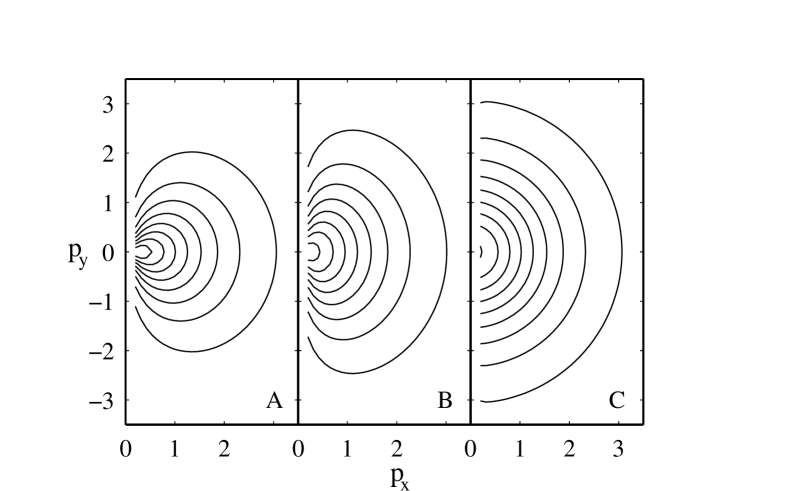
Figure 1: The freeze-out distribution, $f_{free}(x,\vec{p})$, in the rest frame of the freeze out front (RFF) calculated from the model presented in sect. II. The momentum is plotted in units of [T], and $T=m$ is assumed. Contour lines are given at values of 0.9, 0.8, 0.7, … times the maximum of $f_{free}$. Here the center of the Rest Frame of the Gas (RFG) is at rest in RFF, $u_{RFG}^{\mu}=(1,0,0,0)$, however, the Eckart and Landau flow velocities of the frozen out matter do not vanish! The figures A, B, C correspond to $x=0.02\lambda,\ 3\lambda,\ \infty$ respectively. At large distances from the initial point of the freeze out process, $x\longrightarrow\infty$ (C), the distribution becomes a cut Jüttner distribution. The earlier stages of the freeze out are, however, characterized by asymmetric distributions, elongated in the freeze out direction, $x$. This may lead to a large-$p_{t}$ enhancement, compared to the usual Jüttner assumption as freeze out distribution used in most previous calculations.

Let us take first the most simple kinetic model describing the evolution of such a system. Starting from a fully equilibrated Jüttner distribution the two components of the momentum distribution develop according to the coupled differential equations:

$$\partial_{x}f_{int}(x,\vec{p})dx = -\Theta(p^{\mu}d\sigma_{\mu})\frac{\cos\theta_{\vec{p}}}{\lambda}f_{int}(x,\vec{p})dx,$$

$$\partial_{x}f_{free}(x,\vec{p})dx = +\Theta(p^{\mu}d\sigma_{\mu})\frac{\cos\theta_{\vec{p}}}{\lambda}f_{int}(x,\vec{p})dx.$$ (6)

Here the interacting component, $f_{int}$, will deviate from the Jüttner shape and the solution will take the form

$$f_{int}(x,\vec{p})=f_{Juttner}(x=0,\vec{p})\exp\left[-\Theta(p^{\mu}d\sigma_{\mu})\frac{\cos\theta_{\vec{p}}}{\lambda}x\right].$$ (7)

This solution is depleted in the forward $\vec{p}$-direction, particularly along the $x$-axis. Inserting it into the second differential equation above, leads to the freeze out solution:

$$f_{free}(x,\vec{p})=f_{Juttner}(x=0,\vec{p})\left\{1-\exp\left[-\Theta(p^{\mu}d\sigma_{\mu})\frac{\cos\theta_{\vec{p}}}{\lambda}x\right]\right\}.$$ (8)

At $x\longrightarrow\infty$ this distribution will tend to the cut Jüttner distribution introduced in the previous section. (see Figs. 1, 2, and 3.) The remainder of the original Jüttner distribution survives as $f_{int}$, even if $x\longrightarrow\infty$. In this model the particle density does not change with $x$, barely particles moving faster than the freeze out front (i.e. $p^{\mu}d\sigma_{\mu}>0$) are transferred gradually from component $f_{int}$ to component $f_{free}$. This is a highly unrealistic model, indicating that rescattering and re-thermalization should be taken into account in $f_{int}$. This would allow particle transfer from the ”negative momentum part” (i.e. $p^{\mu}d\sigma_{\mu}<0$) of $f_{int}$ to $f_{free}$, which is not possible otherwise.

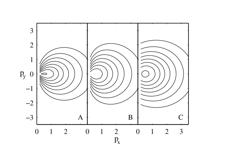
Figure 2: The same as Fig. 1, except here the center of the Rest Frame of the Gas (RFG) is not at rest in RFF, $u_{RFG}^{\mu}=(\gamma,0.5,0,0)$. At large distances from the initial point of the freeze out process, $x\longrightarrow\infty$ (C), the distribution becomes a cut Jüttner distribution, but less than half of the distribution is cut off! Note that the boosted Jüttner distribution became Lorentz elongated and asymmetric (see Fig. 2.10 of ref. [5].) The earlier stages of the freeze out, here also, are characterized by asymmetric distributions, elongated in the freeze out direction, $x$.

III Freeze out distribution with rescattering

The assumption that the interacting part of the distribution remains the distorted (after some drain) Jüttner distribution, is of course highly unrealistic. Rescattering within this component will lead to re-thermalization and re-equilibration of this component. Thus the re-equilibration and the drain terms are in competition and they mutually determine the evolution of the component, $f_{int}$.

To include the collision terms explicitly into the transport equations, (6) leads to a combined set of integro-differential equations. We can, however, take advantage of the relaxation time approximation to simplify the description of the dynamics.

Then the two components of the momentum distribution develop according to the coupled differential equations:

$$\partial_{x}f_{int}(x,\vec{p})dx = -\Theta(p^{\mu}d\sigma_{\mu})\frac{\cos\theta_{\vec{p}}}{\lambda}f_{int}(x,\vec{p})dx$$

$$+ \left[f_{eq}(x,\vec{p})-f_{int}(x,\vec{p})\right]\frac{1}{\lambda^{\prime}}dx,$$

$$\partial_{x}f_{free}(x,\vec{p})dx = +\Theta(p^{\mu}d\sigma_{\mu})\frac{\cos\theta_{\vec{p}}}{\lambda}f_{int}(x,\vec{p})dx.$$ (9)

Here, the interacting component of the momentum distribution shows the tendency to approach an equilibrated, Jüttner type, distribution with a relaxation length coefficient, $\lambda^{\prime}\approx\lambda$. Of course due to the energy, momentum and conserved particle drain, this distribution, $f_{eq}(x,\vec{p})$ is not the same as the initial Jüttner distribution, but its parameters, $n_{eq}(x)$, $T_{eq}(x)$ and $u^{\mu}_{eq}(x)$, change as required by the conservation laws.

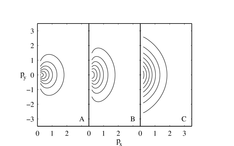
Figure 3: The same as Fig. 1, except here the center of the Rest Frame of the Gas (RFG) is not at rest in RFF, $u_{RFG}^{\mu}=(\gamma,-0.5,0,0)$. At large distances from the initial point of the freeze out process, $x\longrightarrow\infty$ (C), the distribution becomes a cut Jüttner distribution, but more than half of the distribution is cut off! The earlier stages of the freeze out, here also are characterized by asymmetric distributions, but these are not elongated in the freeze out direction, $x$.

Conservation Laws.   In this case the change of the conserved quantities caused by the particle transfer from component $int$ to component $free$ can be obtained in terms of the distribution functions as:

$$dN_{i}^{\mu}=-\frac{dx}{\lambda}\int\frac{d^{3}p}{p_{0}}p^{\mu}\Theta(p^{\mu}d\sigma_{\mu})\cos\theta_{\vec{p}}f_{int}(x,\vec{p})$$

and

$$dT_{i}^{\mu\nu}=-\frac{dx}{\lambda}\int\frac{d^{3}p}{p_{0}}p^{\mu}p^{\nu}\Theta(p^{\mu}d\sigma_{\mu})\cos\theta_{\vec{p}}f_{int}(x,\vec{p}).$$

If we do not have collision or relaxation terms in our transport equation then the conservation laws are trivially satisfied. If, however, collision or relaxation terms are present these contribute, to the change of $T^{\mu\nu}$ and $N^{\mu}$, and this should be considered in the modified distribution function $f_{int}(x,\vec{p})$.

Immediate re-thermalization limit.

As a first approximation to the solution of eqs. (9) let us assume that $\lambda^{\prime}\longrightarrow 0$, i.e. we have immediate re-thermalization after every step $dx$. Thus the drain is always happening from a component of shape $f_{eq}(x,\vec{p})$, with parameters, $\hat{n}(x),\ T(x)$ and $u_{RFG}^{\mu}(x)$, and we can assume that $f_{int}=f_{eq}$ is of spherical Jüttner form at any $x$ including both positive and negative momentum parts. Above and henceforth the notation is similar to the one in [3]: $\tilde{n}=8\pi T^{3}e^{\mu/T}(2\pi\hbar)^{-3}$,  $a={\frac{m}{T}}$,  so that $\hat{n}(\mu,T)=\tilde{n}a^{2}K_{2}(a)/2$ is the invariant scalar density of the symmetric massless Jüttner gas, $b=a/\sqrt{1-v^{2}}$,  $v=d\sigma_{0}/d\sigma_{x}$,  $A=(2+2b+b^{2})e^{-b}$,  and

$${\cal K}_{n}(z,w)\equiv\frac{2^{n}(n)!}{(2n)!}\ z^{-n}\!\!\int_{w}^{\infty}\!\!\!dx\ (x^{2}-z^{2})^{n-1/2}\ \ e^{-x}\ ,$$

i.e. ${\cal K}_{n}(z,z)=K_{n}(z)$.

In this case the change of conserved quantities due to particle drain or transfer can be evaluated for an infinitesimal $dx$. We assume that the 3-flow is normal to the freeze out surface, and for simplicity we assume $v>0$. In this case the change of the conserved particle currents in the RFF is given by

$$\begin{array}[]{rll}dN_{i}^{0}=&-\frac{dx}{\lambda}\frac{\tilde{n}}{4v^{2}\gamma^{2}}\left[bK_{1}(b)+b(3v^{2}-1)\gamma^{2}(2K_{1}(a)-{\cal K}_{1}(a,b))\right.+\\ &&\\ &+\left.\gamma v^{2}b^{2}(2K_{0}(a)-{\cal K}_{0}(a,b))+2v^{3}\gamma^{3}(b+1)e^{-b}\right]\ ,\\ &&\\ dN_{i}^{x}=&-\frac{dx}{\lambda}\frac{\tilde{n}}{4v^{3}\gamma^{3}}\left\{v^{2}(3v^{2}-1)\gamma^{3}b(2K_{1}(a)-{\cal K}_{1}(a,b))+\right.\\ &&\\ &+(2+v^{4}\gamma^{2}b^{2})(2K_{0}(a)-{\cal K}_{0}(a,b))-\\ &&\\ &\left.-2K_{0}(b)+2v\gamma^{2}e^{-b}[v^{2}\gamma^{2}(b+1)+v^{2}b-1]\right\},\end{array}$$

and for the change of the energy - momentum tensor in the RFF we obtain that

$$\begin{array}[]{rll}dT_{i}^{00}=&-\frac{dx}{\lambda}\frac{\tilde{n}T}{4v^{2}\gamma^{2}}\left\{v^{2}\gamma^{2}b^{2}(3+v^{2})(2K_{2}(a)-{\cal K}_{2}(a,b))+\right.\\ &&\\ &+(v^{2}b^{2}-v^{2}-1)\gamma b(2K_{1}(a)-{\cal K}_{1}(a,b))-\\ &&\\ &-b^{2}(2K_{0}(a)-{\cal K}_{0}(a,b))+\frac{a}{\gamma}K_{1}(b)+a^{2}K_{0}(b)+\\ &&\\ &\left.+v\gamma^{2}e^{-b}\!\left[(1{+}3v^{2})\gamma^{2}\!A(b)-(2{+}v^{2}b^{2})(b{+}1)+v^{4}(1{+}\frac{v^{2}}{3})\gamma^{2}b^{3}\right]\right\},\\ &&\\ dT_{i}^{0x}=&-\frac{dx}{\lambda}\frac{\tilde{n}T}{4}\left\{\frac{1+3v^{2}}{v}b^{2}(2K_{2}(a)-{\cal K}_{2}(a,b))+\right.\\ &&\\ &+vab^{2}(2K_{1}(a)-{\cal K}_{1}(a,b))+\left[v^{2}\gamma^{2}b\left(-a^{2}+\frac{1+3v^{2}}{3v}b^{2}\right)-b^{2}+\right.\\ &&\\ &\left.\left.+(v^{2}+3)\gamma^{2}A(b)\right]e^{-b}\right\}-\frac{2T}{v\gamma}dN_{i}^{0}\ ,\end{array}$$

$$\begin{array}[]{rll}dT_{i}^{xx}=&-\frac{dx}{\lambda}\frac{\gamma^{2}\tilde{n}T}{4v}\left\{v(3+v^{2})a^{2}(2K_{2}(a)-{\cal K}_{2}(a,b))+\right.\\ &&\\ &+v^{3}a^{3}(2K_{1}(a)-{\cal K}_{1}(a,b))+\left[\frac{v^{4}}{3}(3+v^{2})b^{3}+\right.\\ &&\\ &\left.\left.+a^{2}(v^{4}b-1)+(3v^{2}+1)A(b)\right]e^{-b}\right\}-\frac{3T}{v\gamma}dN_{i}^{x}\ ,\\ &&\\ dT_{i}^{yy}=&{-}\frac{dx}{\lambda}\frac{\tilde{n}T}{8v^{2}\gamma^{2}}\left[-(v^{2}+1)a(2K_{1}(a)-{\cal K}_{1}(a,b))-\right.\\ &&\\ &\left.-v^{2}a^{2}\left(2K_{0}(a){-}{\cal K}_{0}(a,b)\right)+\frac{a}{\gamma}K_{1}(b)-2v(b{+}1)e^{-b}\right]+\frac{3T}{2v\gamma}dN_{i}^{x}\end{array}$$

and $dT_{i}^{zz}=dT_{i}^{yy}$. Note that in RFF the flow velocity of the re-thermalized component is $u_{i,RFG}^{\mu}(x)=\gamma_{\sigma}(x)\ (1,v(x),0,0)|_{RFF}$, where $\gamma_{\sigma}=1/\sqrt{1-v^{2}}$.

The new parameters of distribution $f_{int}$, after moving to the right by $dx$ can be obtained from $dN_{i}^{\mu}$ and $dT_{i}^{\mu\nu}$. The conserved particle density of the re-thermalized spherical Jüttner distribution after a step $dx$ is

$$\hat{n}_{i}(x+dx)=\hat{n}_{i}(x)+d\hat{n}_{i}(x)=\sqrt{N_{i}^{\mu}(x+dx)N_{i,\mu}(x+dx)}$$

where the expressions are invariant scalars. After straightforward calculation the differential equation describing the change of the proper particle density is:

$$d\hat{n}_{i}(x)=u_{i,RFG}^{\mu}(x)\ dN_{i,\mu}(x)\,.$$ (10)

Although this covariant equation is valid in any frame, we can calculate it in the RFF, where the values of $dN_{i}^{\mu}$s were given above. Note again, that the particle drain from $f_{int}(x)$, described by $dN_{i}^{\mu}$ is constrained to the ”positive part” in the momentum space, but after re-thermalization we attribute this to the change in the complete spherical Jüttner distribution, $f_{int}(x+dx)$. Thus, in order to conserve momentum, we have to obtain a decreased Eckart flow velocity after the infinitesimal particle drain.

For the re-thermalized interacting component Eckart’s flow velocity is the velocity of the RFG, which changes with $x$, so we can actually denote this frame as RFG$(x)$. For the spherical Jüttner distribution the Landau and Eckart flow velocities are the same, $u^{\mu}_{i,E,RFG}(x)=u^{\mu}_{i,L,RFG}(x)=u^{\mu}_{i,RFG}(x)$. Thus we can evaluate the flow velocity $u_{i,RFG}^{\mu}(x+dx)$:

$$u^{\mu}_{i,RFG}(x+dx)=N_{i}^{\mu}(x+dx)/\sqrt{N_{i}^{\mu}N_{i,\mu}}\,,$$

which leads to the following covariant expression

$$du^{\mu}_{i,E,RFG}(x)=\Delta^{\mu\nu}_{i}(x)\ \frac{dN_{i,\nu}(x)}{\hat{n}_{i}(x)}\,,$$ (11)

where $\Delta^{\mu\nu}_{i}(x)=g^{\mu\nu}-u_{i,RFG}^{\mu}(x)\,u_{i,RFG}^{\nu}(x)\,,$  is a projector to the plane orthogonal to $u^{\mu}_{i,RFG}(x)$. This equation is valid in any reference frame, nevertheless we know the four-vectors on the r.h.s. in the RFF explicitly. Then the new flow velocity of the matter evaluated according to Eckart’s definition is $u^{\mu}_{i,E,RFG}(x+dx)$ $=$ $u^{\mu}_{i,RFG}(x)$ $+$ $du_{i,E,RFG}^{\mu}(x)$.

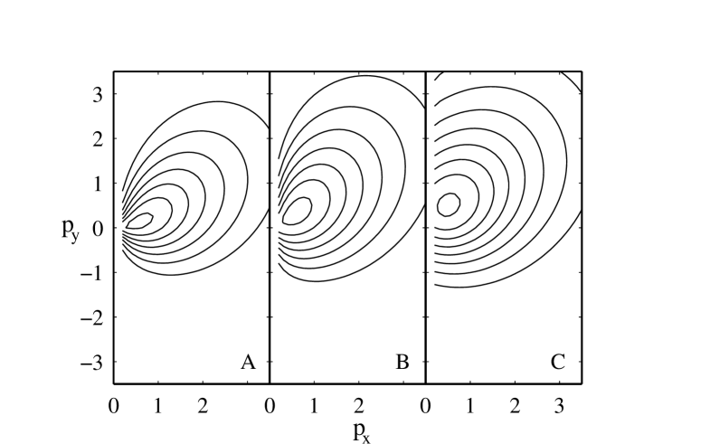
Figure 4: The same as Fig. 1, except here the center of the Rest Frame of the Gas (RFG) is not at rest in RFF, $u_{RFG}^{\mu}=(\gamma,0.5,0.5,0)$. At large distances from the initial point of the freeze out process, $x\longrightarrow\infty$ (C), the distribution becomes a cut Jüttner distribution, which is not centralized in $p_{y}$ and less than half of the distribution is cut off! The earlier stages of the freeze out, here also are characterized by distributions asymmetric both in the directions $p_{x}$ and $p_{y}$, and these are also elongated in the direction of the freeze out flow velocity, $u_{RFG}^{\mu}$.

To get the temperature and the change of Landau’s flow velocity, we have to analyze the change of the energy momentum tensor. Before the particle drain the energy - momentum tensor at $x$ in the RFG is diagonal, $T^{\mu\nu}_{i}(x)={\rm diag}(e_{i},P_{i},P_{i},P_{i})|_{RFG(x)}$ while in the RFF $T^{\mu\nu}_{i}(x)$ $=$ $\left[(e_{i}+P_{i})\right.$ $u_{i,RFG}^{\mu}u_{i,RFG}^{\nu}(x)$ $\left.-P_{i}g^{\mu,\nu}\right]|_{RFF(x)}$. Adding the drain terms, $dT^{\mu\nu}_{i}(x)$, to this arising from the freeze out while we move to the right by $dx$, yields $T^{\mu\nu}_{i}(x+dx)$ which will not be diagonal in the RFG$(x)$ and the pressure part will not be isotropic. We can Lorentz transform this to another frame which diagonalizes $T^{\mu\nu}_{i}(x+dx)$. This means to find the Landau flow velocity of the new system, $u^{\mu}_{i,L,RFG}(x+dx)$ in the original RFG$(x)$. After a straightforward diagonalization, a somewhat tricky algebra and neglecting second and higher order terms we arrive at the covariant expression

$$du^{\mu}_{i,L,RFG}(x)=\frac{\Delta^{\mu\nu}_{i}(x)\ \ dT_{i,\nu\sigma}\ \ u^{\sigma}_{i,RFG}(x)}{e_{i}+P_{i}}.$$ (12)

Although, for the spherical Jüttner distribution the Landau and Eckart flow velocities are the same, the change of this flow velocity when calculated from the baryon current and from the energy current are different

$$du^{\mu}_{i,E,RFG}(x)\neq du^{\mu}_{i,L,RFG}(x)\,.$$

This is a clear consequence of the asymmetry caused by the freeze out process as we pointed out already at the discussion of the properties of the cut Jüttner distribution. Unfortunately, this also illustrates the weakness of our assumption on the complete re-thermalization to a spherical Jüttner distribution, because we cannot choose the correct velocity change: If we choose $du^{\mu}_{E}$ as the new velocity of the (spherical Jüttner distribution) $f_{int}(x+dx)$, then we violate the momentum conservation in our model, on the other hand if we choose $du^{\mu}_{L}$, then we violate the baryon current conservation! Thus a spherical (or even elliptic) distribution cannot be fitted to the freeze out drain, and we would have to use an ansatz, which has (in addition) an asymmetry in the $x$ direction (i.e., an egg shape), for the distribution $f_{int}$.

Being aware of this weakness of the model, we nevertheless, maintain the assumption of spherical Jüttner shape for $f_{int}$ for the sake of simplicity. We can choose the flow velocity change then according to the physical problem. For example for the freeze out of baryon free plasma this problem does not occur, and we have to choose $du^{\mu}_{L}$.

The last item is to determine the change of the temperature parameter of $f_{int}$. From the relation $e\equiv u_{\mu}T^{\mu\nu}u_{\nu}$ we readily obtain the expression for the change of energy density

$$de_{i}(x)=u_{\mu,i,RFG}(x)\ \ dT^{\mu\nu}_{i}(x)\ \ u_{\nu,i,RFG}(x)\,,$$ (13)

and from the relation between the energy density and the temperature (see Chapter 3 in ref.[5]), we can obtain the new temperature at $x+dx$. Fixing these parameters we fully determined the spherical Jüttner approximation for $f_{int}$. With this ansatz the pressure asymmetry and pressure balance cannot be realized, thus our model will be only a rather approximate description of the freeze out process.

Nevertheless, we can draw some preliminary conclusions about the development of the kinetic distribution during freeze-out.

IV Conclusions

We turned to the problem of estimating the freeze out distribution. Obviously the real freeze out distribution depends strongly on the details of the freeze out (and hadronization) dynamics. In heavy ion reactions, the curvature of the freeze out surface and the conditions varying in time do affect the freeze out distribution, nevertheless, as a first step, we assumed that the process is stationary and the curvature of the front is negligible. These approximations are extreme, but still enable us to draw some preliminary conclusions.

Following the lines and ideas presented in ref. [3], the first simple kinetic freeze out model reproduces the cut Jüttner distribution as the limiting distribution, $f_{free}$, after complete freeze out at large distances. However, the model at the same time leads to unrealistic consequences, namely that the interacting part of the distribution, $f_{int}$ also survives fully, as the other part of the Jüttner distribution. Thus having both components at the end in this model, the physical freeze out is actually not realized. This turns out to be a consequence of the fact that the effect of rescattering and thermalization in the interacting part of the distribution was ignored.

In an improved but still rather approximate kinetic freeze out model which takes rescatterings into account, the interacting component is assumed to be instantly re-thermalized taking a spherical Jüttner shape at each time step with changing parameters. The model leads to a set of coupled differential equations (10,11,12,13). Equations (11) and (12) can be used in some combined form, or one of them can be selected which fits the physical situation the best. Then the three parameters of the interacting component, $f_{int}$, can be obtained in each time step analytically (considering ${\cal K}_{n}(x,y)$ an analytic function).

Now the density of the interacting component will gradually decrease and disappear according to eq. (10), the flow velocity will also decrease in both cases, (11) or (12), because only forward going particles freeze out, and the energy density will decrease also according to eq. (13). Thus, the initial contribution to $f_{free}$ at small $x$ will resemble the distribution shown in Fig. 2A, then as $x$ increases and the velocity decreases it will become to similar to Fig. 1B, while at the final stages it will approach Fig. 3C. As a consequence the integrated distribution will not resemble a cut Jüttner distribution.

Thus the arising post freeze out distribution, $f_{free}$ will be a superposition of cut Jüttner type of components, from a series of gradually slowing down Jüttner distributions. This will lead to a comet shaped final momentum distribution, with a more dominant leading head and a tail. In these rough models a large fraction ($\sim 95\%$) of the matter is frozen out by $x=3\lambda$, thus the distribution $f_{free}$ at this distance can be considered as a first estimate of the post freeze out distribution. One should also keep in mind that the models presented here do not have realistic behavior in the limit $x\longrightarrow\infty$, due to their one dimensional character. Nevertheless, this improved model with rescattering enables complete freeze out (unlike the simpler model in sect. II where only the originally forward moving particles freeze out even at large distances).

In case of rapid hadronization of QGP and simultaneous freeze out, the idealization of a freeze out hypersurface may be justified, however, an accurate determination of the post freeze out hadron momentum distribution would require a nontrivial dynamical calculation.

References

- [1] A.H. Taub, Phys. Rev. 74 (1948) 328.
- [2] L.P. Csernai, Sov. JETP 65 (1987) 216; Zh. Eksp. Theor. Fiz. 92 (1987) 379.
- [3] Cs. Anderlik, L.P. Csernai, F. Grassi, Y. Hama, T. Kodama, and Zs. Lázár, nucl-th/9806004.
- [4] F. Cooper and G. Frye, Phys. Rev. D 10 (1974) 186.
- [5] L.P. Csernai: Introduction to Relativistic Heavy ion Collisions (Wiley, 1994)
- [6] Yu.M. Sinyukov, Sov. Nucl. Phys. 50 (1989) 228; and Z. Phys. C43 (1989) 401.
- [7] K.A. Bugaev, Nucl. Phys. A606 (1996) 559.
- [8] L.V. Bravina, I.N. Mishustin, N.S. Amelin, J.P. Bondorf and L.P. Csernai, Phys. Lett. B354 (1995) 196.
- [9] J.J. Neumann, B. Lavrenchuk and G. Fai, Heavy Ion Phys. 5 (1997) 27.