The Stability of the Spectator, Dirac, and Salpeter Equations for Mesons

Abstract

Mesons are made of quark-antiquark pairs held together by the strong force. The one channel spectator, Dirac, and Salpeter equations can each be used to model this pairing. We look at cases where the relativistic kernel of these equations corresponds to a time-like vector exchange, a scalar exchange, or a linear combination of the two. Since the model used in this paper describes mesons which cannot decay physically, the equations must describe stable states. We find that this requirement is not always satisfied, and give a complete discussion of the conditions under which the various equations give unphysical, unstable solutions.

I Introduction

A Background

In the simplest models, mesons are bound states of a valance quark-antiquark pair confined by the strong force. Even for such a simple case a covariant model is needed when the mesons are composed of light quarks with high momentum components. However, covariant models require knowledge of the Lorentz structure of the confining interaction, and it turns out that some choices of Lorentz structure for some equations will produce mesons which decay. When no mechanism for decay has been included in the model (which will be the situation for the cases discussed in this paper), this is a sign that the solutions are unphysical. In may be acceptable for an equation to produce unstable (i.e. unphysical) solutions /it if these solutions are confined to a region of the spectrum which can be precisely characterized and systematically ignored, but if this is not possible equations which produce such unphysical solutions are unsatisfactory. In this paper we study confining potentials with scalar and time-like vector exchanges, and find that the stability of such interactions depends on the kind of relativistic equation used for the description of the interaction.

This is not the first time that the stability of covariant models of confinement has been addressed. Several papers have been written on this topic, some with contradictory conclusions. Two examples which illustrate this are papers titled An exact argument against an effective vector exchange for the confining quark-antiquark potential [1], and Evidence against a scalar confining potential in QCD [2]. If both papers are correct, this would indicate that, at best, the Lorentz structure for the potential is more complex than a simple scalar or vector exchange.

Our research into the question of stability was motivated by the paper of Parramore and Piekarewicz[3], which found that the Salpeter equation was stable when the vector strength exceeded the scalar strength. This seemed counter intuitive to us, since it is well known that, because of the famous Klein paradox, the Dirac equation is stable only when the potential is predominately scalar. Their result also contradicted the work of another group [4] who found that the Salpeter equation was stable for a pure scalar confining interaction, provided the quark mass was sufficiently large.

FIG. 1.: Example of electroweak decay of the $\rho^{+}$ meson.

FIG. 2.: Example of strong decay of the $\rho^{+}$ meson.

B Physical and unphysical instabilities

We begin the discussion by making a distinction between instabilities which are physical and those which are unphysical. Real mesons have a finite lifetime and can decay either through the strong interaction or the electroweak interaction. For example, the $\rho^{+}$ can decay into a photon and a $\pi^{+}$ through the electroweak interaction shown in Fig. 1. It can also decay into a $\pi^{+}$ and $\pi^{0}$ via the strong interaction, as shown in Fig. 2. In this paper we describe mesons which are isolated from external influences (including vacuum fluxuations), and use an equation which excludes the electroweak interaction and does not include any mechanism for the production of quark-antiquark pairs. Hence both of these decay mechanisms are excluded from the theory and thus the mesons described by our equations cannot decay physically. Therefore any instability emerging from these equations will be unphysical, and a sign that the equations are describing unacceptable states.

C Unphysical instabilities – an example

The Dirac equation for a linear combination of a scalar and vector confining potential provides a familiar example of the kind of unphysical instabilities we are discussing. Consider the Dirac equation for the linear confining potential $V(r)=\sigma\,r\left\{(1-y)+y\gamma^{0}\right\}$

$$E_{B}\gamma^{0}\phi(r)=(m+V(r)+{\bf\gamma}\cdot{\bf\nabla})\;\phi(r)\\$$ (1)

where $\sigma$ and the vector strength $y$ are both constants. The solutions of this equation have both positive and negative binding energy eigenvalues $E_{B}$. If the system described by this equation could interact with the outside world (e.g. absorb or emit photons), the positive energy states could decay to negative energy states (unless all of the negative energy states were occupied as in hole theory). However, we have assumed that there is no coupling to the outside world, and hence this equation should describe a stable system, even if some of the binding energy eigenvalues are infinitely large and negative. However, it is well known that the Dirac equation does not give stable solutions for all values of the vector strength $y$ and we review this result now.

FIG. 3.: Sketch of the solution to the Dirac equation for the scalar case, where $\sigma>0$ and $y=0$.

FIG. 4.: Sketch of the solution to the Dirac equation for the vector case, where $\sigma>0$ and $y=1$.

The nature of the solutions to the Dirac equation can be studied by looking at the expectation value of $U=m+V$. The form of this expectation value, which describes how the wave function behaves, is

$$\langle U\rangle_{\pm}=\cases{m+\sigma\,r&positive energy\cr-m-\sigma\,r(1-2y)\qquad&negative energy}$$ (2)

where the positive energy expectation value is a matrix element involving $u$-type positive energy spinors, $\langle U\rangle_{+}=\bar{u}Uu$, and the negative energy expectation value is a matrix element involving $v$-type negative energy spinors, $\langle U\rangle_{-}=\bar{v}Uv$. The result (2) comes from the matrix elements

$$\bar{u}u= 1 =-\bar{v}v$$ (3)

$$\bar{u}\gamma^{0}u= 1 =\bar{v}\gamma^{0}v\,,$$ (4)

which hold when the total momentum $p=0$. When Eq. (2) is sketched for pure scalar ($y=0$) or pure vector ($y=1$) cases, Fig. 3 and Fig. 4 are produced, respectively. The resulting wave functions for a particle with energy $E$ are sketched on the figures, along with the form of $\langle U\rangle$ which produces it.

To understand these results, first neglect the coupling between positive and negative energy states. Then the positive energy states move under the influence of the potential $\langle U\rangle_{+}$ and the negative energy states under the influence of $\langle U\rangle_{-}$. For the scalar case ($y=0$), the choice $\sigma>0$ produces confinement for both positive and negative energy states. Coupling the two solutions does not change this picture significantly, and the exact solution is a total wave function which drops to zero at large distances. This means that both positive and negative energy solutions describe particles permanently confined around the point $r=0$.

Next look at the vector case ($y=1$), and begin again by neglecting the coupling between the positive and negative energy states. In this case, however, either the positive or negative energy state is always unconfined. For the example shown in Fig. 4, $\sigma>0$ and the positive energy states are confined and the negative energy states are not. Including coupling between the positive and negative energy states mixes the two states, and the wave function for the exact positive energy solution acquires a component with a “tail” which oscillates to infinity, signaling deconfinement. The effect of the coupling is to produce an effective potential composed of two regions separated by a finite potential barrier through which the quark can tunnel. Once it is free of the potential barrier it can propagate endlessly through space, thus becoming a free quark. In this case, the exact coupled solutions do not confine either the positive or negative energy states, and the bound state is unstable. This example, known as the Klein paradox [5], is one of the unphysical instabilities we are trying to avoid.

D Requirements for stability

A relativisitic equation with a confining kernel with a given Lorentz structure will have stable, physical solutions only if the following four conditions are satisfied:

(1) the binding energy must be real;

(2) the energy eigenvalues must be independent of the numerical approximations used to obtain them;

(3) unphysical solutions, if there are any, must be confined to an identifiable part of the spectrum clearly separated from the physical solutions; and

(4) the solutions must have the correct structure in coordinate or momentum space.

We will discuss each of these conditions in turn.

Condition 1 – real energies. Any eigenstate wave function which describes a meson in momentum space, $\psi({\bf p},t)$, can be written

$$\psi({\bf p},t)=\phi({\bf p})e^{-iEt}\,,$$ (5)

where $E=\sqrt{\mu^{2}+{\bf P}\,^{2}}$. The discussion is simplified if the particle is chosen to be at rest, ${\bf P}=0$. Then, if $\mu$ is complex, $\mu=\mu_{0}\pm i\Gamma/2$, the absolute square of the meson wave function is

$$|\psi(p,t)|^{2}=|\phi(p)|^{2}e^{\pm\Gamma t}\,.$$ (6)

As time increases, this goes exponentially either to zero or to infinity, showing that the state is unstable.

Condition 2 – numerical stability. The different relativistic equations will be solved numerically in Sec. IV using spline functions to model the wavefunctions in momentum space. (A description of the properties of the spline functions is given in Appendix A.) So long as enough spline functions are used to model the system, the energy of the lower lying stable states will not vary much as the spline rank is increased. However, if the state is unstable it is part of a continuous spectrum and the energies obtained from the “eigenvalue” equation only represent a discrete approximation to this continuous spectrum. They will vary strongly with the number of splines, much as the location of the $n$th point in the interval $[0,1]$ will vary strongly with the number of intervals $N$ into which the the line segment is divided. This dependence of an energy level on spline rank is one of the most obvious symptoms of instability.

Condition 3 – isolation of instabilities. In some cases we find that, following the second criteria, the positive energy states are stable and the negative energy states are unstable. This may be acceptable for a phenomenology, where the negative energy states can be rejected as unphysical from the start. However, in some cases these unstable negative energy states become positive as the spline number increases, and they can become so positive that they cross the gap separating the negative and positive energy states, enter the positive energy spectrum, and mix with states which would otherwise be stable. In this case the distinction between (stable) positive energy states and (unstable) negative energy states becomes blurred, and we cannot rely on the predictions of the equation.

Condition 4 – correct structure. Even if the mass is real, the state might not be confined in a finite region of coordinate space (as in the Dirac example outlined above). If the state is confined, its coordinate space wave function will approach zero as $r\to\infty$ faster than an exponential. It can be shown that the momentum space wave function resulting from such a state will also fall off at $p\to\infty$ faster than an exponential, and that the number of nodes will correspond to the level of the state. It is easy to distinguish such behavior from that of an unconfined state, which is neither localized in coordinate nor momentum space, and which has many nodes not related to the level of the state. We can use the Dirac wave functions for comparison, since we know that they are stable for scalar confinement and unstable for vector confinement. Examples of both types of states will be given in Sec. IV.

In the following sections, these stability conditions will sometimes be referred to by number, as we will see that a successful phenomenology requires that all of them be satisfied.

E Summary and Outline

In summary, the stability conditions are: (1) the eigenvalues of the system must be real; (2) the eigenvalues cannot vary with the spline rank; (3) the positive energy states must always be greater than any unstable negative energy states; and (4) the wave functions must have the appropriate structure for that specific state.

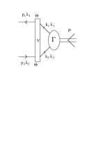
FIG. 5.: Feynman diagram for the meson bound state vertex function. The kernel, or potential, is denoted by $V$.

In Sec. II specific forms are given for the Dirac, Salpeter, and one channel spectator (denoted 1CS) relativistic equations. Then in Sec. III these three equations are studied using an approximation technique which gives insight into the origin of the instabilities, and the estimated masses of stable states are compared to the exact numerical solutions presented in Sec. IV. The three equations are solved numerically in Sec. IV using spline functions for a quasirelativistic confining potential. The actual equations used in the computer code and the properties of spline functions are given in Appendix A. Finally, conclusions are given in Sec. V.

II The Relativistic Equations

In this section we define the one-channel spectator (1CS) equation obtained by confining the heavier particle 1 (assumed to be the quark) to its positive energy mass shell, fixing the $k_{0}$ integration. Then we show that these equations reduce to the Dirac equation for the lighter particle (particle 2) in the limit when the mass of the heaver particle $m_{1}\to\infty$. We conclude by finding a helicity representation for the 1CS and for the Salpeter equation.

A Dirac form for the one-channel spectator equation

The Feynman diagram for the bound state meson vertex is shown in Fig. 5. Particle 1 is the quark, particle 2 the antiquark, and $\Theta$ is a matrix in Dirac space which describes how the confining force couples to the quark or antiquark. It can be a scalar, $\openone$, or the time component of a four-vector, $\gamma^{0}$. The kernel $V$ contains the momentum dependent structure of the confining potential. The equations are derived in the center of mass rest frame, $P=(\mu,{\bf 0})$. Later, the quark will be placed on shell, thus producing the single channel equation. The four momenta used in the diagram are

$$p_{1}= p+\textstyle{\frac{1}{2}}P\qquad\;p_{2} =p-\textstyle{\frac{1}{2}}P$$ (7)

$$k_{1}= k+\textstyle{\frac{1}{2}}P\qquad\;k_{2} =k-\textstyle{\frac{1}{2}}P\,.$$ (8)

The vector $k$ is the average internal momentum and vector $p$ is the average external momentum of the quark-antiquark pair:

$$p=\textstyle{\frac{1}{2}}(p_{1}+p_{2})\qquad P=p_{1}-p_{2}\,.$$ (9)

With this notation, the Bethe-Salpeter equation [6] for the bound state vertex function for the meson is

$$\Gamma(p)=i\int\frac{d^{4}k}{(2\pi)^{4}}\;V(p,k)\;\Theta\;\frac{m_{1}+\not{k}_{1}}{m_{1}^{2}-k_{1}^{2}}\;\Gamma(k)\;\frac{m_{2}+\not{k}_{2}}{m_{2}^{2}-k_{2}^{2}}\;\Theta\,.$$ (10)

FIG. 6.: This figure shows the position of the four poles associated with the four propagators $G^{\rho}_{i}$ in the bound state equations.

The two fermion propagators have poles in the complex $k_{0}$ plane; these four poles are shown Fig. 6. Factoring the denominators of the propagators

$$\frac{1}{m_{i}^{2}-k_{i}^{2}}=G_{i}^{+}\,G_{i}^{-}$$ (11)

the poles are at

$$\begin{array}[]{lll}{\rm pole\;\;1}&(G^{+}_{1})^{-1}=E_{k_{1}}-(k_{0}+\frac{1}{2}\mu)-i\epsilon=0&k_{0}=E_{k_{1}}-\frac{1}{2}\mu-i\epsilon\cr{\rm pole\;\;3}&(G^{-}_{1})^{-1}=E_{k_{1}}+(k_{0}+\frac{1}{2}\mu)-i\epsilon=0&k_{0}=-E_{k_{1}}-\frac{1}{2}\mu+i\epsilon\cr{\rm pole\;\;2}&(G^{+}_{2})^{-1}=E_{k_{2}}-(k_{0}-\frac{1}{2}\mu)-i\epsilon=0&k_{0}=E_{k_{2}}+\frac{1}{2}\mu-i\epsilon\cr{\rm pole\;\;4}&(G^{-}_{2})^{-1}=E_{k_{2}}+(k_{0}-\frac{1}{2}\mu)-i\epsilon=0&k_{0}=-E_{k_{2}}+\frac{1}{2}\mu+i\epsilon\,.\cr\end{array}$$ (12)

To place particle 1 on the positive energy mass shell, the $k_{0}$ integration is closed in the lower half plane and only the residue from pole 1 is kept. This gives the following equation:

$$\Gamma(p)=-\int\frac{d^{3}k}{2E_{k_{1}}(2\pi)^{3}}\;V(p,k)\;\Theta\;(m_{1}+\not{\hat{k}}_{1})\;\Gamma(k)\;\frac{m_{2}+\not{k}_{2}}{m_{2}^{2}-k_{2}^{2}}\;\Theta\,,$$ (13)

where now $\hat{k}_{1}=(E_{k_{1}},{\bf k})$ and $k_{2}=(E_{k_{1}}-\mu,{\bf k})$. This is one form of the one channel spectator equation.

Next, we recall that the projection operator can be written [7] as a sum over on-shell $u$ spinors (to be defined below)

$$m_{1}+\not{\hat{k}}_{1}=\sum_{\lambda^{\prime}}u({\bf k},\lambda^{\prime})\overline{u}({\bf k},\lambda^{\prime})\,.$$ (14)

Therefore, if we define the relativistic meson wave function by

$$\Psi(k,\lambda)=\frac{1}{\sqrt{2E_{k_{1}}}}\;\overline{u}({\bf k},\lambda)\;\Gamma(k)\;\frac{m_{2}+\not{k}_{2}}{m_{2}^{2}-k_{2}^{2}}$$ (15)

then Eq. (13) becomes

$$\Psi(p,\lambda)\,(m_{2}-\not{p_{2}})=-\int\frac{d^{3}k}{(2\pi)^{3}}\;\frac{V(p,k)}{\sqrt{4E_{p_{1}}E_{k_{1}}}}\;\sum_{\lambda^{\prime}}\Theta^{++}_{\lambda\lambda^{\prime}}(p,k)\;\Psi(k,\lambda^{\prime})\;\Theta\,,$$ (16)

where

$$\Theta^{++}_{\lambda\lambda^{\prime}}(p,k)=\overline{u}({\bf p},\lambda)\;\Theta\;u({\bf k},\lambda^{\prime})\,.$$ (17)

Equation (16) is the Dirac form of the one-channel spectator equation. Later we will reduce this equation further, but as written in (16) it looks very much like a Dirac equation for the light antiparticle (particle 2) moving under the influence of a effective potential which depends on the spin of the heavy quark. To make this comparison more familiar, we convert the equation into the usual form by taking the transpose and multiplying by the Dirac charge conjugation matrix $C$ (see Ref. [7]). This gives

$$(m_{2}+\not{p}_{2})\,\hat{\Psi}(p,\lambda)=-\hat{\Theta}\,\sum_{\lambda^{\prime}}\int\frac{d^{3}k}{(2\pi)^{3}}\;\hat{\Psi}(k,\lambda^{\prime})\;\frac{V(p,k)}{\sqrt{4E_{p_{1}}E_{k_{1}}}}\;\Theta^{++}_{\lambda\lambda^{\prime}}(p,k)\,,$$ (18)

where

$$\hat{\Psi}(p,\lambda)=C\,\Psi^{\rm T}(p,\lambda)\qquad\hat{\Theta}=C\Theta^{\rm T}C^{-1}\,.$$ (19)

With the exceptions of the spin dependence of the source, expressed through the factor $\Theta^{++}_{\lambda\lambda^{\prime}}(p,k)$, and the fact that the effective potential does not depend solely on ${\bf q}={\bf p}-{\bf k}$, the difference of the three momenta, Eq. (18) looks like the familiar Dirac equation for a particle with four momentum equal to $-p_{2}$ (as expected from the charge conjugate state).

We will now calculate the matrix element $\Theta^{++}$ and show that Eq. (18) does indeed reduce to a Dirac equation in the limit $m_{1}\to\infty$. In spin space the $u$ spinor, as defined in Ref. [7], is

$$u({\bf p},s)=(E_{p}+m)^{\frac{1}{2}}\left(\begin{array}[]{c}\openone\\ \\ \displaystyle{\frac{{\bf\sigma}\cdot{\bf p}}{E_{p}+m}}\end{array}\right)\chi^{s}\,,$$ (20)

which contains the operator ${\bf\sigma}\cdot{\bf p}$. It is convenient to work in helicity space, where ${\bf\sigma}\cdot{\bf p}\,\chi^{\lambda}=2\lambda|{\bf p}|\chi^{\lambda}$. The $u$ spinor in helicity space is therefore

$$u^{+}({\bf p},\lambda_{j})\equiv u({\bf p},\lambda_{j})=N_{p_{j}}\left(\begin{array}[]{c}\openone\\ \\ 2\lambda_{j}\tilde{p}_{j}\end{array}\right)\chi^{\lambda_{j}},$$ (21)

where we have introduced the notation $u^{\rho}$ with $\rho$-spin $=+1$ for the positive energy solutions ($u$) and $\rho$-spin $=-1$ for the negative energy solutions ($v$, described below), and

$$N_{p_{j}}=(E_{p_{j}}+m_{j})^{\frac{1}{2}}\qquad\tilde{p}_{j}=\frac{|{\bf p}|}{N_{p_{j}}^{2}}\,.$$ (22)

The index $j$ denotes a quark $(j=1)$ or antiquark $(j=2)$. The values of $\tilde{p}$ range from 0 to 1. The helicity spinors are defined in Table I for cases when the momentum is along the z axis (external quarks), and when the momentum is in the $xz$ plane at an angle $\theta$ with respect to the z axis. We will use a prime to distinguish the latter from the former. The $v$ spinor, or negative $\rho$-spin state, used in this paper is

$$u^{-}({\bf p},\lambda_{j})\equiv v(-{\bf p},\lambda_{j})=N_{p_{j}}\left(\begin{array}[]{c}-2\lambda_{j}\tilde{p}_{j}\\ \\ \openone\end{array}\right)\chi^{\lambda_{j}}\,,$$ (23)

and is consistent with that used in Ref. [8]. It is convenient to use the helicity representation because helicity is invariant under rotations, and because the vector operator ${\bf\sigma}\cdot{\bf p}$ is replaced by scalar eigenvalues, thus simplifying the algebra.

TABLE I.: Helicity spinors

external quarks	internal quarks
$\lambda_{i}=\phantom{-}\frac{1}{2}$   $\left(\begin{array}[]{c}1\\ 0\end{array}\right)$	$\lambda^{\prime}_{i}=\phantom{-}\frac{1}{2}$   $\left(\begin{array}[]{c}\cos\frac{\theta}{2}\\ \\ \sin\frac{\theta}{2}\end{array}\right)$
$\lambda_{i}=-\frac{1}{2}$   $\left(\begin{array}[]{c}0\\ 1\end{array}\right)$	$\lambda^{\prime}_{i}=-\frac{1}{2}$   $\left(\begin{array}[]{c}-\sin\frac{\theta}{2}\\ \\ \cos\frac{\theta}{2}\end{array}\right)$

The matrix element $\Theta^{++}_{\lambda\lambda^{\prime}}(p,k)$ is then

$$\Theta^{++}_{\lambda\lambda^{\prime}}(p,k)=N_{p_{1}}N_{k_{1}}\Delta_{\lambda\lambda^{\prime}}(\theta^{\prime}\theta)\,\left(1\mp 4\lambda^{\prime}\lambda\,\tilde{p}_{1}\tilde{k}_{1}\right)\,,$$ (24)

where the upper sign is for the scalar vertex and the lower sign for the time-like vector case. We will assume, for the time being, that the polar angle of the external quark is $\theta^{\prime}$ instead of 0 (as it will be later). Then

$$\Delta_{\lambda\lambda^{\prime}}(\theta^{\prime}\theta)=\delta_{\lambda\lambda^{\prime}}\,\cos{\textstyle{1\over 2}}(\theta-\theta^{\prime})-2\lambda\,\delta_{\lambda,\,-\!\lambda^{\prime}}\,\sin{\textstyle{1\over 2}}(\theta-\theta^{\prime})\,.$$ (25)

Therefore, forming the two independent linear combinations

$$\Phi^{+}(p)= \hat{\Psi}\left(p,{\textstyle{1\over 2}}\right)\cos{\textstyle{1\over 2}}\theta^{\prime}-\hat{\Psi}\left(p,-{\textstyle{1\over 2}}\right)\sin{\textstyle{1\over 2}}\theta^{\prime}$$ (26)

$$\Phi^{-}(p)= \hat{\Psi}\left(p,{\textstyle{1\over 2}}\right)\sin{\textstyle{1\over 2}}\theta^{\prime}+\hat{\Psi}\left(p,-{\textstyle{1\over 2}}\right)\cos{\textstyle{1\over 2}}\theta^{\prime}$$ (27)

Eq. (18) becomes

$$(m_{2}+\not{p}_{2})\,{\Phi}^{+}(p)=-\hat{\Theta}\, \int\frac{d^{3}k}{(2\pi)^{3}}\;\frac{N_{p_{1}}N_{k_{1}}}{\sqrt{4E_{p_{1}}E_{k_{1}}}}\,V(p,k)$$ (29)

$$\left\{{\Phi}^{+}(k)\left[1\mp\tilde{p}_{1}\tilde{k}_{1}\cos(\theta-\theta^{\prime})\right]\mp{\Phi}^{-}(k)\;\tilde{p}_{1}\tilde{k}_{1}\sin(\theta-\theta^{\prime})\right\}$$

$$(m_{2}+\not{p}_{2})\,{\Phi}^{-}(p)=-\hat{\Theta}\, \int\frac{d^{3}k}{(2\pi)^{3}}\;\frac{N_{p_{1}}N_{k_{1}}}{\sqrt{4E_{p_{1}}E_{k_{1}}}}V(p,k)$$ (31)

$$\left\{{\Phi}^{-}(k)\left[1\mp\tilde{p}_{1}\tilde{k}_{1}\cos(\theta-\theta^{\prime})\right]\pm{\Phi}^{+}(k)\;\tilde{p}_{1}\tilde{k}_{1}\sin(\theta-\theta^{\prime})\right\}\,.$$

Hence the interaction depends only on the difference $\theta-\theta^{\prime}$ and we may set $\theta^{\prime}=0$ without loss of generality.

For later use we will record here the other $\rho$-spin matrix elements of $\Theta$

$$\Theta^{--}_{\lambda\lambda^{\prime}}(p,k)= \mp\Theta^{++}_{\lambda\lambda^{\prime}}(p,k)$$ (33)

$$\Theta^{+-}_{\lambda\lambda^{\prime}}(p,k)= -N_{p_{1}}N_{k_{1}}\Delta_{\lambda\lambda^{\prime}}(\theta^{\prime}\theta)\,\left(2\lambda^{\prime}\,\tilde{k}_{1}\pm 2\lambda\,\tilde{p}_{1}\right)=\pm\Theta^{-+}_{\lambda\lambda^{\prime}}(p,k)\,.$$ (34)

B Limits of the one-channel spectator equation

Now we can observe that taking the limit $m_{1}\to\infty$ gives a Dirac equation for the light particle. The fixed source for the Dirac equation is a heavy quark, so the equation will model a $Q\,\bar{q}$ system, such as a $D$ meson. As $m_{1}\to\infty$, $\tilde{p}_{1}\to 0$ and $V(p,k)\to V({\bf p}-{\bf k})$ (see below), giving

$$(m_{2}-\not\!{p^{\prime}}_{2})\,{\Phi}(p)=-\hat{\Theta}\,\int\frac{d^{3}k}{(2\pi)^{3}}\;V({\bf p}-{\bf k}){\Phi}(k)\,,$$ (35)

where the helicity of the heavy particle was dropped because the equation is independent of it and we introduced the physical momentum $p_{2}^{\prime}=-p_{2}=(\mu-E_{p_{1}},-{\bf p})\to(E_{B},{\bf p^{\prime}})$, with $E_{B}=\mu-m_{1}$. In position space Eq. (35) is

$$(m_{2}-E_{B}\gamma^{0}+i\,\gamma^{i}\partial_{i})\,{\Phi}({\bf r})=-\hat{\Theta}\;V({\bf r}){\Phi}({\bf r})\,,$$ (36)

We will return to this equation in the next subsection.

The confining potential ${V}({\bf r})$ which appears in Dirac Eq. (36) is taken to be a simple linear potential in position space [9]

$$V(r)=\sigma r=\lim_{\epsilon\rightarrow 0}\sigma re^{-\epsilon r}=\lim_{\epsilon\rightarrow 0}\sigma\frac{d^{2}}{d\epsilon^{2}}\frac{e^{-\epsilon r}}{r}.$$ (37)

In momentum space this potential is

$$V({\bf q})=-8\pi\sigma\lim_{\epsilon\rightarrow 0}\left\{\frac{1}{({\bf q}^{2}+\epsilon^{2})^{2}}-\frac{4\epsilon^{2}}{({\bf q}^{2}+\epsilon^{2})^{3}}\right\}.$$ (38)

This form of the potential is inconvenient because the limit $\epsilon\to 0$ must be taken numerically. For the Dirac equation, we use an alternative form which has the same physics

$$V({\bf q})=-{8\pi\sigma}\left\{\frac{1}{{\bf q}^{4}}-\delta^{3}({q})\int\frac{d^{3}q^{\prime}}{{\bf q}^{\prime 4}}\right\}$$ (39)

where ${\bf q}={\bf p}-{\bf k}$ and ${\bf q}^{\prime}={\bf p}-{\bf k}^{\prime}$. It is instructive to note that the position space form of each of the terms in (39) is

$$-\frac{8\pi\sigma}{{\bf q}^{4}} =\lim_{\epsilon\rightarrow 0}-\frac{8\pi\sigma}{({\bf q}^{2}+\epsilon^{2})^{2}}\rightarrow\lim_{\epsilon\rightarrow 0}-\sigma\frac{e^{-\epsilon r}}{\epsilon}\simeq-\frac{\sigma}{\epsilon}+\sigma r+\cdots$$ (40)

$$\delta^{3}({q})\int d^{3}q^{\prime}\frac{8\pi\sigma}{{\bf q}^{\prime 4}} =\lim_{\epsilon\rightarrow 0}\delta^{3}({q})\int d^{3}q^{\prime}\frac{8\pi\sigma}{({\bf q}^{2}+\epsilon^{2})^{2}}\rightarrow\frac{\sigma}{\epsilon}\,.$$ (41)

Hence the role of the delta function subtraction is to remove the infinite constant from the first term, leaving a pure linear potential.

In relativistic two-body equations, the potential (39) is generalized to [9]

$$V(p,k)=-{8\pi\sigma}\left\{\frac{1}{(p-k)^{4}}-E_{p_{1}}\,\delta^{3}(p-k)\int\frac{d^{3}k^{\prime}}{E_{k^{\prime}_{1}}\,(p-k^{\prime})^{4}}\right\}\,.$$ (42)

The insertion of the energy factors is necessary to make the kernel (42) covariant, and is associated with the restriction of the heavy quark to its mass-shell[9]. The full 1CS also includes the covariant replacement $(p-k)^{2}\to(E_{p_{1}}-E_{k_{1}})^{2}-({\bf p}-{\bf k})^{2}$, but in both the theoretical and numerical studies in this paper we have neglected retardation and use the simplest replacement $(p-k)^{2}\to-({\bf p}-{\bf k})^{2}$. We will refer to this as the quasirelativistic approximation, and it should be emphasized that we use this approximation in this paper only to simplify the discussion. We also neglect the regularization factor and form factor introduced in previous studies [9].

The energy factor in the subtraction term in (42) gives rise to a relativistic effect of some importance. To see this, evaluate the diagonal matrix element

$$\left<\psi|V_{C}|\psi\right> =\int d^{3}p\,d^{3}k\,\psi(p)\left\{E_{p_{1}}\,\delta^{3}(p-k)\int\frac{d^{3}k^{\prime}\,8\pi\sigma}{E_{k^{\prime}_{1}}\,(p-k^{\prime})^{4}}\right\}\psi(k)$$ (43)

$$= \int\frac{d^{3}r\,d^{3}r^{\prime}}{(2\pi)^{3}}\,d^{3}p\,\psi(r^{\prime})e^{i{\bf p}\cdot({\bf r}^{\prime}-{\bf r})}\left\{E_{p_{1}}\int\frac{d^{3}k^{\prime}\,8\pi\sigma}{E_{k^{\prime}_{1}}\,(p-k^{\prime})^{4}}\right\}\psi(r)$$ (44)

$$= \int d^{3}r\psi(r)\left\{E_{p_{1}}\int\frac{d^{3}k^{\prime}\,8\pi\sigma}{E_{k^{\prime}_{1}}\,(p-k^{\prime})^{4}}\right\}\psi(r)\,,$$ (45)

where, in the last line, $p=\sqrt{p^{2}}\to\sqrt{-\nabla^{2}}$. Hence the subtraction term becomes an operator which is a function of $p^{2}\to-\nabla^{2}$ but independent of $r$. It can be evaluated by standard means

$$E_{p_{1}}\int\frac{d^{3}k^{\prime}\,8\pi\sigma}{E_{k^{\prime}_{1}}\,(p-k^{\prime})^{4}}= \lim_{\epsilon\rightarrow 0}E_{p_{1}}\int\frac{d^{3}k^{\prime}\,8\pi\sigma}{E_{k^{\prime}_{1}}\,[(p-k^{\prime})^{2}+\epsilon^{2}]^{2}}$$ (46)

$$= \frac{\sigma}{\epsilon}-\frac{2\sigma}{\pi m_{1}}\left\{\frac{m_{1}}{E_{p_{1}}}+\frac{m_{1}^{3}}{pE_{p_{1}}^{2}}\log\left(\frac{E_{p_{1}}+p}{m_{1}}\right)\right\}$$ (47)

$$= \frac{\sigma}{\epsilon}-C(p^{2})\,.$$ (48)

This new subtraction term contains the same singular part we found before [see Eq. (41)] plus a new finite part $C(p^{2})$. The finite part arises from the relativistic energy factor in Eq. (48), which produces an infinitesimal modification of the singular part, and it vanishes in the $m_{1}\to\infty$ limit. It has an interesting effect which will be discussed in the next subsection.

The confining potential has the property that it is very singular when ${\bf q}\to 0$. This suggests using a peaking approximation in which $\theta\simeq\theta^{\prime}$, so that the coupling between $\Phi^{+}$ and $\Phi^{-}$ can be neglected. No further approximations are needed, because we may reduce all factors of $E_{p_{1}}$ and $E_{k_{1}}$ to derivative operators, and replace

$$\tilde{k}_{1}\tilde{p}_{1}\cos(\theta-\theta^{\prime})= \frac{{\bf k}\cdot{\bf p}}{(E_{k_{1}}+m_{1})(E_{p_{1}}+m_{1})}$$ (49)

$$\to -\frac{({\bf k}-{\bf p})^{2}}{2(E_{k_{1}}+m_{1})(E_{p_{1}}+m_{1})}+\frac{\tilde{k}_{1}^{2}}{2}+\frac{\tilde{p}_{1}^{2}}{2}\,,$$ (50)

because the operators $k^{2}$ (which operates on the initial wave functions) and $p^{2}$ (which operates on the final wave functions) will eventually give indentical results. Furthermore, the operator ${\bf q}^{2}$ can be reduced to

$$\frac{8\pi\sigma{\bf q}^{2}}{2{\bf q}^{4}}=\frac{4\pi\sigma}{{\bf q}^{2}}\to\frac{\sigma}{r}\,.$$ (51)

Combining all of these effects, Eq. (LABEL:der11f) becomes a single Dirac-like equation with a momentum dependent potential

$$(m_{2}+\not\!{p}_{2})\,{\Phi}(p)= \hat{\Theta}C(p)\Phi(p)-\hat{\Theta}\,\int\frac{d^{3}k}{(2\pi)^{3}}\;V(p,k){\cal N}{\Phi}(k)$$ (53)

$$\times\left[1\mp\frac{1}{2}(\tilde{k}_{1}^{2}+\tilde{p}_{1}^{2})\pm\frac{1}{2}\frac{{\bf q}^{2}}{(E_{k_{1}}+m_{1})(E_{p_{1}}+m_{1})}\right]\,,$$

where ${\cal N}={N_{p_{1}}N_{k_{1}}}/\sqrt{4E_{p_{1}}E_{k_{1}}}$. Recalling that $p_{20}=M-E_{p_{1}}=E_{B}+m_{1}-E_{p_{1}}$, the coordinate space form of this equation is

$$\left(m_{2}-\left[E_{B}+m_{1}-\sqrt{m_{1}^{2}-\nabla^{2}}\right]\;\gamma^{0}+i\,\gamma^{i}\partial_{i}\right)\,{\Phi}({\bf r})$$ (54)

$$\qquad=-\hat{\Theta}\left(\left[\sigma r-C(p^{2})\right]\left(1\mp\tilde{p}^{2}_{1}\right)\mp\frac{\sigma}{r}\frac{1}{(E_{1}+m_{1})^{2}}\right){\cal N}{\Phi}({\bf r})\,,$$ (55)

where we have anticipated the application to diagonal matrix elements where $k^{2}=p^{2}\to-\nabla^{2}$, and all functions $E_{p_{1}}=E_{1}$ are replaced by $\sqrt{m_{1}^{2}-\nabla^{2}}$. Using Eq. (55) we can study the single-channel spectator equation when the mass $m_{1}$ is close to $m_{2}$, and also see how it approaches the Dirac limit. We will study these issues approximately in Sec. III.

C Equations with mixed scalar and vector confinement

Note that the operator ${\Theta}$ depends on its Dirac structure; it is $\openone$ for a scalar confinement and $\gamma^{0}$ for vector confinement. Hence Eq. (19) gives

$$\hat{\Theta}=\cases{\phantom{-}\openone&\qquad{\rm scalar}\cr-\gamma^{0}&\qquad{\rm vector}\, .}$$ (56)

In the nonrelativistic limit, the Dirac equation reduces to a Schrödinger equation for the upper component, and we will choose the sign of our potential so that it confines the positive energy solution in the nonrelativistic limit. Hence, in order to obtain a nonrelativistic confining potential equal to $\sigma r$, independent of the mixing parameter $y$, the operator form ${\cal O}$ of a mixed kernel must be

$${\cal O}=(1-y)\,\openone\,\otimes\,\openone-y\,\gamma^{0}\,\otimes\,\gamma^{0}\,.$$ (57)

Using this definition and the result Eq. (55) gives the following equation for a mixed confining potential

$$\left(m_{2}-\left[E_{B}+m_{1}-E_{1}\right]\;\gamma^{0}+i\,\gamma^{i}\partial_{i}\right)\,{\Phi}({\bf r})$$ (58)

$$\qquad=-\hat{\Theta}\left(\left[\sigma r-C(p^{2})\right]\left(1-\tilde{p}^{2}_{1}(1-2y)\right)-\frac{\sigma}{r}\frac{(1-2y)}{(E_{1}+m_{1})^{2}}\right){\cal N}{\Phi}({\bf r})\,.$$ (59)

Assuming a ground state solution of the form [7]

$${\Phi}({\bf r})=\left(\matrix{f(r)\cr-ig(r)\sigma\cdot{\bf\hat{r}}}\right)\chi\,,$$ (60)

Eq. (59) reduces to the following set of coupled equations for the radial wave functions $f(r)$ and $g(r)$

$$\left(E_{B}-m_{2}-\left[E_{1}-m_{1}\right]\right)\,f\,+\,\frac{dg}{dr}+\frac{2}{r}g$$ (61)

$$\qquad=\left((\sigma r-C)\left[1-\tilde{p}^{2}_{1}\,(1-2y)\right]-\frac{\sigma}{r}\frac{(1-2y)}{(E_{1}+m_{1})^{2}}\right){\cal N}\,f$$ (62)

$$\left(E_{B}+m_{2}-\left[E_{1}-m_{1}\right]\right)\,g\,-\,\frac{df}{dr}$$ (63)

$$\qquad=-\left((\sigma r-C)\left[(1-2y)-\tilde{p}^{2}_{1}\right]-\frac{\sigma}{r}\frac{1}{(E_{1}+m_{1})^{2}}\right){\cal N}\,g\,.$$ (64)

We will return to this coupled set of equations in the next section.

D Spectator equation in helicity space

The equations we have obtained so far are convenient for approximate analysis, but an exact helicity decomposition is better for numerical solutions. To obtain this form of the one-channel spectator equation, return to Eq. (16) and expand the wave function and the projection operator in terms of the helicity spinors given in Eqs. (21) and (23). The wave function can be expanded using the decomposition of the propagator into $\rho$ spin contributions [7],

$$\frac{(m_{2}+\not{k}_{2})}{m_{2}^{2}-k_{2}^{2}}=\frac{1}{2E_{k_{2}}}\sum_{\lambda_{2}}\left[\frac{u({\bf k},\lambda_{2})\bar{u}({\bf k},\lambda_{2})}{E_{k_{2}}-k_{20}-i\epsilon}-\frac{v(-{\bf k},\lambda_{2})\bar{v}(-{\bf k},\lambda_{2})}{E_{k_{2}}+k_{20}-i\epsilon}\right]\,.$$ (65)

Using this in Eq. (15) shows that the wave function has the form

$$\Psi(p,\lambda)=\sum_{\rho\lambda_{2}}\Psi^{\rho}_{\lambda\lambda_{2}}(p)\,\overline{u}^{\rho}({\bf p},\lambda_{2})\,.$$ (66)

Furthermore, the most general form of the pseudoscalar vertex function with particle 1 on shell is

$$\overline{u}^{+}({\bf p},\lambda)\,\Gamma(p)=\overline{u}^{+}({\bf p},\lambda)\;\left\{\Gamma_{1}\,\gamma^{5}+\Gamma_{2}\,\gamma^{5}\,\left(m_{2}-\not\!{p}_{2}\right)\right\}\,,$$ (67)

and these Dirac operators are built only from the $2\times 2$ matrices $\openone$ and $\sigma\cdot{\bf p}=2\lambda p$. Therefore in helicity space the helicity is conserved and an explicit calculation shows that

$$\overline{u}^{+}({\bf p},\lambda)\,\Gamma(p)\,u^{\rho}({\bf p},\lambda_{2})=\delta_{\lambda\lambda_{2}}\,(2\lambda)^{\delta_{+\rho}}\,\Gamma^{\rho}(p)\,,$$ (68)

where the $\Gamma^{\rho}(p)$ are independent of the helicity. Hence the expansion (66) can be written

$$\sqrt{2E_{p_{2}}}\,\Psi(p,\lambda)=\frac{1}{\sqrt{4E_{p_{2}}E_{p_{1}}}}\left\{\psi_{1a}(p)\,\overline{u}^{-}({\bf p},\lambda)+(2\lambda)\,\psi_{1b}(p)\,\overline{u}^{+}({\bf p},\lambda)\right\}\,,$$ (69)

where

$$\psi_{1a}=-\frac{\Gamma^{-}}{E_{k_{2}}+E_{k_{1}}-\mu} \psi_{1b}=\frac{\Gamma^{+}}{E_{k_{2}}-E_{k_{1}}+\mu},$$ (70)

Bringing all of these elements together, using Eq. (34), and choosing the sign of the vector interaction in accordance with Eq. (57) gives the helicity form of the single channel spectator equation

$$\left(\begin{array}[]{c}(E_{B}-E_{p_{2}}-[E_{p_{1}}-m_{1}])\,\psi_{1a}(p)\\ (E_{B}+E_{p_{2}}-[E_{p_{1}}-m_{1}])\,\psi_{1b}(p)\\ \end{array}\right)=\int_{\bf{k}}\overline{V}\,\pmatrix{D_{1}&D_{2}\cr D_{3}&D_{4}\cr}\left(\begin{array}[]{c}\psi_{1a}(k)\\ \psi_{1b}(k)\\ \end{array}\right)\,,$$ (71)

where $E_{B}=\mu-m_{1}$,

$$\int_{\bf{k}}=\int\frac{d^{3}k}{(2\pi)^{3}}\;,$$ (72)

the rescaled potential kernel is

$$\overline{V}=\frac{N_{p_{1}}N_{p_{2}}N_{k_{1}}N_{k_{2}}}{4\sqrt{E_{p_{1}}E_{p_{2}}E_{k_{1}}E_{k_{2}}}}\;V\,,$$ (73)

and $D_{i}=A_{i}+B_{i}\cos\theta$ with

$$\begin{array}[]{ll}A_{1}=Q&B_{1}=\mp R\cr A_{2}=T_{2}&B_{2}=\pm S_{2}\cr A_{3}=S_{2}&B_{3}=\pm T_{2}\cr A_{4}=R&B_{4}=\mp Q\,,\end{array}$$ (74)

and

$$\begin{array}[]{ll}Q=1+\tilde{p}_{1}\tilde{p}_{2}\tilde{k}_{1}\tilde{k}_{2}&R=\tilde{p}_{1}\tilde{k}_{1}+\tilde{p}_{2}\tilde{k}_{2}\cr S_{j}=\tilde{p}_{j}-\tilde{k}_{1}\tilde{k}_{2}\tilde{p}_{j^{\prime}}&T_{j}=\tilde{k}_{j}-\tilde{p}_{1}\tilde{p}_{2}\tilde{k}_{j^{\prime}}\,.\end{array}$$ (75)

In (74) the upper sign holds for scalar confinement and the lower for vector confinement and in (75) $j^{\prime}\neq j$.

For the mixed scalar/vector confinement defined in Eq. (57) the values of $A_{i}$ and $B_{i}$ are:

$$\begin{array}[]{ll}A_{1}=Q&B_{1}=-R(1-2y)\cr A_{2}=T_{2}&B_{2}=S_{2}(1-2y)\cr A_{3}=S_{2}&B_{3}=T_{2}(1-2y)\cr A_{4}=R&B_{4}=-Q(1-2y)\,.\end{array}$$ (76)

When the masses are equal this equation reduces to the equation previously introduced in Ref. [10].

E Dirac equation in helicity space

The helicity form of the Dirac equation is obtained from (71) by taking the $m_{1}\to\infty$ limit

$$\left(\begin{array}[]{c}(E_{B}-E_{p_{2}})\,\psi_{1a}(p)\\ (E_{B}+E_{p_{2}})\,\psi_{1b}(p)\\ \end{array}\right)=\int_{\bf{k}}\bar{V}\,\pmatrix{d_{1}&d_{2}\cr d_{3}&d_{4}\cr}\left(\begin{array}[]{c}\psi_{1a}(k)\\ \psi_{1b}(k)\\ \end{array}\right)\,,$$ (77)

where now $\bar{V}=VN_{p_{2}}N_{k_{2}}/\left(2\sqrt{E_{p_{2}}E_{k_{2}}}\,\right)$ and $d_{i}=a_{i}+b_{i}\cos\theta$ with

$$\begin{array}[]{ll}a_{1}=1&b_{1}=-\tilde{p}_{2}\tilde{k}_{2}(1-2y)\cr a_{2}=\tilde{k}_{2}&b_{3}=\tilde{p}_{2}(1-2y)\cr a_{3}=\tilde{p}_{2}&b_{2}=\tilde{k}_{2}(1-2y)\cr a_{4}=\tilde{p}_{2}\tilde{k}_{2}&b_{1}=-(1-2y)\,.\end{array}$$ (78)

We conclude this section with a derivation of the helicity form of the Salpeter equation.

F Salpeter equation in helicity space

The Salpeter [11] uses the approximation that the potential, or kernel, of the Bethe-Salpeter equation is independent of $k_{0}$ and $p_{0}$. Therefore, in coordinate space the potentials and the wave functions are instantaneous, i.e. $t_{1}=t_{2}$. The Salpeter Equation has two undesirable features. First, neglecting the energy dependence of the kernel is unphysical. Second, there is no Dirac limit for this equation. When the mass of one of the particles is taken to infinity, the resulting equations do not reduce to a Dirac equation for the light quark moving in the field created by the heavy quark. Hence, it is most appropriate to use this equation for equal masses, far away from the one body limit.

The direct derivation of the Salpeter equation utilizes the same steps as those used for the 1CS equation with a few modifications. In this case pole 2, as defined in Eq. (12) and Fig. 6, must be included. For brevity we will only give the final result. The general equation is

$$\Gamma^{\rho_{1}\rho_{2}}_{1}(p)=\int\frac{d^{3}k}{(2\pi)^{3}}V_{11}^{\prime}\sum_{\rho_{1}^{\prime}\rho_{2}^{\prime}}\sum_{\lambda_{1}^{\prime}\lambda_{2}^{\prime}}\Theta_{1}^{\rho_{1}\rho_{1}^{\prime}}\Gamma_{1}^{\rho_{1}^{\prime}\rho_{2}^{\prime}}G_{2}^{\rho_{2}^{\prime}}\Theta_{2}^{\rho_{2}^{\prime}\rho_{2}}$$ (79)

where $\rho_{1}\neq\rho_{2}$ and $\rho_{1}^{\prime}\neq\rho_{2}^{\prime}$. The second channel wave function, denoted $\psi_{2a}$, corresponds to propagation of the two quarks in their negative energy state, and is equal to

$$\psi_{2a}=-\frac{\Gamma^{-+}_{1}}{E_{k_{2}}+E_{k_{1}}+\mu}\,.$$ (80)

The two wave functions, $\psi_{1a}$ and $\psi_{2a}$ satisfy the coupled equations

$$\left(\begin{array}[]{c}(\mu-E_{p_{2}}-E_{p_{1}})\psi_{1a}(p)\\ (\mu+E_{p_{2}}+E_{p_{1}})\psi_{2a}(p)\\ \end{array}\right)=\int_{\vec{k}}\overline{V}\,\pmatrix{D_{1}&-D_{5}\cr D_{5}&-D_{1}\cr}\left(\begin{array}[]{c}\psi_{1a}(k)\\ \psi_{2a}(k)\\ \end{array}\right)\,,$$ (81)

with

$$D_{5}=\tilde{p}_{1}\tilde{p}_{2}+\tilde{k}_{1}\tilde{k}_{2}+(1-2y)\left(\tilde{p}_{1}\tilde{k}_{2}+\tilde{p}_{2}\tilde{k}_{1}\right)\cos\theta$$ (82)

All other terms have the same definitions as before.

III Approximate theoretical results

In this section we develop approximations which help us understand the stability issues which will arise when the equations are solved numerically.

A Dirac solutions for large $r$

We begin by studying the stability of Eq. (64) in the Dirac limit when $m_{1}\to\infty$

$$E_{B}\,f=\left(m_{2}+\sigma r\right)\,f-\frac{dg}{dr}-\frac{2}{r}g$$ (83)

$$E_{B}\,g=\left(-m_{2}-\sigma r(1-2y)\right)\,g+\frac{df}{dr}\,.$$ (84)

This is the exact Dirac equation for a potential which is a superposition of scalar and vector linear confining forces. At large $r$ the equations become approximately

$$\sigma r\,f-\frac{dg}{dr} =0$$ (85)

$$-\sigma r(1-2y)\,g+\frac{df}{dr} =0\,.$$ (86)

The solution to these equations depends on the value of $y$. If $y<1/2$, then the solution which approaches zero as $r\to\infty$ is

$$f(r)=N_{f}\,e^{-\sqrt{1-2y}\;\frac{1}{2}\sigma r^{2}}\qquad g(r)=N_{g}\,e^{-\sqrt{1-2y}\;\frac{1}{2}\sigma r^{2}}\,,$$ (87)

where

$$N_{f}=-\sqrt{1-2y}\;N_{g}\,.$$ (88)

Note that the wave functions become less confined as $y\to 1/2$. For $y>1/2$ the solutions are oscillatory and escape to large $r$. In this case the most general solution is a linear combination of the following two independent solutions

$$f_{1}(r)= N_{f_{1}}\,\sin\left(\sqrt{2y-1}\;\frac{1}{2}\sigma r^{2}\right)\qquad g_{1}(r)=N_{g_{1}}\,\cos\left(\sqrt{2y-1}\;\frac{1}{2}\sigma r^{2}\right)$$ (89)

$$f_{2}(r)= N_{f_{2}}\,\cos\left(\sqrt{2y-1}\;\frac{1}{2}\sigma r^{2}\right)\qquad g_{2}(r)=N_{g_{2}}\,\sin\left(\sqrt{2y-1}\;\frac{1}{2}\sigma r^{2}\right)\,,$$ (90)

where

$$N_{f_{1}} =-\sqrt{2y-1}\;N_{g_{1}}$$ (91)

$$N_{f_{2}} =\sqrt{2y-1}\;N_{g_{2}}\,.$$ (92)

This is the simple mathematical explanation behind the results shown in Figs. 3 and 4.

B Estimates for the one-channel spectator equation

Study of the solutions of the approximate one channel spectator equation, Eq. (64), is complicated by the presence of the operators $\sqrt{m_{1}^{2}-\nabla^{2}}$ and $\tilde{p}_{1}^{2}$. We will therefore develop a variational-like method which can give us insight into the confining behavior of the equation.

First, if $\sigma=0$ the exact solution of the equations is

$$f(r)= f_{o}\,j_{0}(\gamma r)$$ (93)

$$g(r)= g_{o}\,j_{1}(\gamma r)\,,$$ (94)

where $j_{\ell}$ is the spherical Bessel function of order $\ell$, and the energy is a function of the parameter $\gamma$

$$E_{B}(\gamma)=\left[\sqrt{m_{1}^{2}+\gamma^{2}}-m_{1}\right]\pm\sqrt{m_{2}^{2}+\gamma^{2}}\,.$$ (95)

The spectrum is continous with a gap between the positive and negative energy states. It is amusing to see that the energies of both the positive and negative energy states are always greater than the corresponding Dirac state energies, and that the negative energy spectrum is now bounded between $-m_{2}$ and $-m_{1}$, instead of running from $-m_{2}$ to $-\infty$. This already illustrates one of the new features of the 1CS equation.

When $\sigma\neq 0$ we cannot solve the equation analytically, and will limit our study to the behavior of the expectation value of the energies as estimated by taking matrix elements of the equation. To compute these matrix elements we will use wave functions of the type shown in Fig. 7, which are constructed from spherical bessel functions of order zero and one. This choice makes the evaluation of functions of the operator $\nabla^{2}$ easy.

Ideally, the functions used should consist of a region where $-\nabla^{2}$ is positive, and a “tail” region where $-\nabla^{2}<0$. The functions shown in Fig. 7 were constructed from $j_{\ell}(\gamma r)$ and $h_{\ell}(kr)$ joined so that the function and its first derivative are continuous. However, we found that the contributions from the tails did not change the qualitative behavior of the matrix elements, and hence we present here only the simplest results for wave functions without tails (where $k/\gamma\to\infty$, the heavy solid lines in the figure). These results are easy to evaluate.

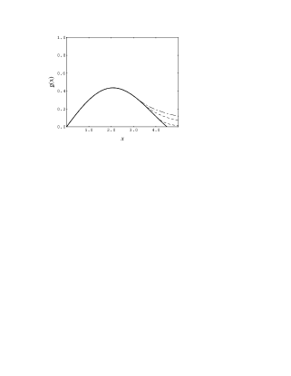
FIG. 7.: The trial wave functions $f(x)$ and $g(x)$ as a function of $x=\gamma r$. The different tails are for the cases $k/\gamma$ = 0.1 (biggest tail), 0.5, and 2.0 (smallest tail), as discussed in the text.

Hence the “trial” wave functions we choose are

$$f(r)= \cases{f_{o}\,j_{0}(\gamma r)&$\gamma r<\pi$\cr 0\qquad\qquad\qquad&$\gamma r>\pi$}$$ (96)

$$g(r)= \cases{g_{o}\,j_{1}(\gamma r)&$\gamma r<n_{1}$\cr 0\qquad\qquad\qquad&$\gamma r>n_{1}$\, ,}$$ (97)

where $j_{\ell}$ is the spherical Bessel function of order $\ell$, $\gamma$ is a variational parameter, and the constant $n_{1}=4.493$ is the location of the zero of $j_{1}$. These wave functions are eigenfunctions of the operator $\nabla^{2}$:

$$\nabla^{2}\,f(r) =\frac{1}{r}\frac{\partial^{2}}{\partial r^{2}}\,r\,f(r)=-\gamma^{2}\;f(r)$$ (98)

$$\nabla^{2}\,g(r) =\left(\frac{1}{r}\frac{\partial^{2}}{\partial r^{2}}\,r-\frac{2}{r^{2}}\right)\,g(r)=-\gamma^{2}\;g(r)\,\,.$$ (99)

Hence the operators $\sqrt{m_{1}^{2}-\nabla^{2}}$ and $\tilde{p}_{1}^{2}$ can be readily calculated.

FIG. 8.: The Dirac energy $E=E_{B}$ as a function of the variational parameter $\gamma$ for different mixing ratios $y=0$ (solid line), $y=0.4$ (dot-dashed), $y=0.6$ (dashed), and $y=1.0$ (dotted).

FIG. 9.: Energies $E=E_{B}$ as a function of the variational parameter $\gamma$ for the Dirac equation (solid line) and the 1CS equation with $m_{1}=10m_{2}$ (dashed line). In both cases, $y=0$.

FIG. 10.: The 1CS energy $E=E_{B}$ as a function of the variational parameter $\gamma$ for different mass ratios $\kappa=m_{1}/m_{2}=10$ (solid line), $\kappa=5$ (dot-dashed), $\kappa=2$ (dashed), and $\kappa=1$ (dotted). In all cases, $y=0$

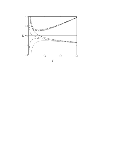
FIG. 11.: The 1CS energy $E=E_{B}$ as a function of the variational parameter $\gamma$ for different mixing ratios $y=0$ (solid line), $y=0.4$ (dot-dashed), $y=0.6$ (dashed), and $y=1.0$ (dotted). In all cases $m_{1}/m_{2}=10$.

FIG. 12.: As in Fig. 11 but with $m_{1}=m_{2}$.

Substituting $f$ and $g$ into Eq. (64), multiplying the first equation by $j_{0}(\gamma r)$ and the second by $j_{1}(\gamma r)$, and integrating over $d^{3}r$ gives the following coupled equations for $f_{o}$ and $g_{o}$

$$\left(E_{B}-\left[\sqrt{m_{1}^{2}+\gamma^{2}}-m_{1}\right]-m_{2}\right)\,f_{o}+\gamma\,g_{o}$$ (100)

$$\qquad\qquad=\left\{\left(\frac{\sigma c_{1}}{\gamma}-C(\gamma^{2})\right)\left(1-\tilde{p}^{2}_{1}\,(1-2y)\right)-\frac{\sigma c_{2}}{\gamma}\tilde{p}^{2}_{1}\,(1-2y)\right\}\,{\cal N}\,f_{o}\equiv S_{f}\,f_{o}$$ (101)

$$\left(E_{B}-\left[\sqrt{m_{1}^{2}+\gamma^{2}}-m_{1}\right]+m_{2}\right)\,g_{o}-\gamma\,b\,f_{o}$$ (102)

$$\qquad\qquad=-\left\{\left(\frac{\sigma c_{3}}{\gamma}-C(\gamma^{2})\right)\left(1-2y-\tilde{p}_{1}^{2}\right)-\frac{\sigma c_{4}}{\gamma}\tilde{p}^{2}_{1}\right\}\,{\cal N}\,g_{o}\equiv-S_{g}\,g_{o}\,,$$ (103)

where

$$\begin{array}[]{ll}c_{1}={\displaystyle\frac{\int_{0}^{\pi}x^{3}dxj_{0}^{2}(x)}{\int_{0}^{\pi}x^{2}dxj_{0}^{2}(x)}=1.571}&c_{3}={\displaystyle\frac{\int_{0}^{n_{1}}x^{3}dxj_{1}^{2}(x)}{\int_{0}^{n_{1}}x^{2}dxj_{1}^{2}(x)}=2.659}\cr&\cr c_{2}={\displaystyle\frac{\int_{0}^{\pi}xdxj_{0}^{2}(x)}{\int_{0}^{\pi}x^{2}dxj_{0}^{2}(x)}=0.776}&c_{4}={\displaystyle\frac{\int_{0}^{n_{1}}xdxj_{1}^{2}(x)}{\int_{0}^{n_{1}}x^{2}dxj_{1}^{2}(x)}=0.412}\end{array}$$ (104)

and

$$b={\displaystyle\frac{\int_{0}^{\pi}x^{2}dxj_{1}^{2}(x)}{\int_{0}^{n_{1}}x^{2}dxj_{1}^{2}(x)}=0.734}\,.$$ (105)

Solving Eq. (103) gives an estimate for the eigenvalues $E_{B}$ as a function of $\gamma$, related to the size of the state

$$E_{B}=\sqrt{m_{1}^{2}+\gamma^{2}}-m_{1}+{1\over 2}(S_{f}-S_{g})\pm\sqrt{{1\over 4}(2m_{2}+S_{f}+S_{g})^{2}+\gamma^{2}\,b}\,,$$ (106)

where $S_{f}$ and $S_{g}$ were defined in Eq. (103). These energy surfaces for a variety of cases are shown in Figs. 8–12. In all of these cases we chose $\sigma=0.2$ GeV² and $m_{2}=0.325$ GeV. We will now discuss some of the interesting features of these solutions.

TABLE II.: Comparison of the exact and estimated solutions for the Dirac and 1CS equations. All energies are in GeV, and the symbol – indicates that there is no stable solution.

parameters		positive energy			negative energy
		exact	estimate		exact	estimate
$m_{1}/m_{2}$	$y\;$	$E_{1}$	$E$	$\gamma\;$	$E_{-1}$	$E$	$\gamma\;$
Dirac
$\infty$	0.0	0.976	0.950	0.715	-1.249	-1.226	0.859
	0.4	1.028	1.014	0.673	-0.660	-0.650	0.463
One Channel Spectator
10	0.0	0.964	0.946	0.635	-1.091	-1.034	0.988
	0.4	1.013	1.007	0.603	-0.619	-0.598	0.505
5	0.0	0.940	0.926	0.579	-0.936	-0.828	1.272
	0.4	0.992	0.992	0.552	-0.548	-0.532	0.563
2	0.0	0.857	0.857	0.471	-0.607	–	–
	0.4	0.928	0.952	0.452	–	–	–
1	0.0	0.745	0.777	0.379	-0.330	–	–
	0.4	0.853	0.928	0.367	–	–	–

Note that the solutions (106) are always real, and that as $\gamma\to 0$

$$E_{B}\to\frac{\sigma}{2\gamma}\left(c_{1}-c_{3}(1-2y)\pm|c_{1}+c_{3}(1-2y)|\right)$$ (107)

Hence the positive energy solution always approaches $+\infty$ as $\gamma\to 0$, but the negative energy solution goes like

$$E_{B}^{-}\to\frac{\sigma}{\gamma}\displaystyle{\cases{-c_{3}(1-2y)&if $y<0.795=\displaystyle{\frac{c_{1}+c_{3}}{2c_{3}}}$\cr&\cr c_{3}(2y-1)\qquad&if $y>0.795\,,$\cr}}$$ (108)

and becomes positive for $y>1/2$, as shown in Figs. 11 and 12. This is a sign of instability. When $y>1/2$ the positive energy states cannot be stable because they may always reduce their energy by tunneling through to a negative energy surface and sliding down to $-\infty$.

A similar problem may occur at large $\gamma$, but because our estimates are less reliable here (we neglected the wave function tails which are more important at large $\gamma$) we can draw no firm conclusion. As $\gamma\to\infty$,

$$E_{B} \to\gamma\left(1\pm\sqrt{b}\right)\,,$$ (109)

and because $b<1$ the negative energy solutions also become positive at large $\gamma$. This feature sets in at lower values of $\gamma$ as the mass ratio $m_{1}/m_{2}$ decreases, as is shown in Fig. 10. In fact we do note that the numerical solutions for the negative energy states are unstable for small values of $m_{1}/m_{2}$, but we see no sign of instability in the positive energy solutions for small values of $y$ and all values of $m_{1}/m_{2}$.

Finally, a comparison between these estimates and exact solutions for the ground state are summarized in Table II. Note that Eq. (64) does a credible job of explaining the trends, all of which can be understood qualitatively from examination of the figures.

Before leaving the discussion of the 1CS equation, we comment on two features of our estimates due to the presence of the “constant” term $C(p^{2})$ of relativistic origin [recall Eq. (48)]. First, note that the positive energy 1CS solutions approach the Dirac limit as $m_{1}\to\infty$ from below instead of from above, as would have been suggested by our analysis of the free particle case. (Note the comparison in Fig. 9.) Even though the energy factor $\left[E_{1}-m_{1}\right]$ is positive, the term $C$ is negative and is just a bit larger, giving the observed behavior. Second, the term $-C$ becomes more negative with decreasing mass ratio, explaining the drop in the binding energy as $m_{1}/m_{2}$ decreases to unity.

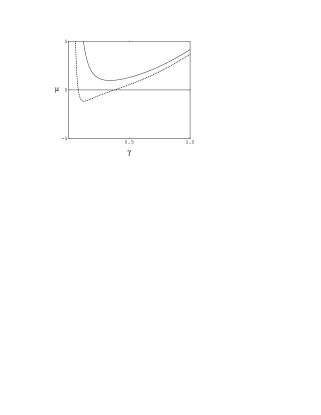
FIG. 13.: The square of the bound state mass $\mu^{2}$ as a function of the parameter $\gamma$ for the Salpeter equation with a pure scalar confining interaction ($y=0$). Solid curve ($m=0.325$), dashed curve ($m=0.1$).

C Stability of the Salpeter equation

Applying our technique to the Salpeter equation (81) for equal masses ($m_{1}=m_{2}=m$) gives

$$\left(\mu-2E\right)\,f_{1}= w_{1}\,f_{1}+w_{2}\,f_{2}$$ (110)

$$\left(\mu+2E\right)\,f_{2}= -w_{1}\,f_{2}-w_{2}\,f_{1}$$ (111)

where

$$w_{1}=\left\{\left(\frac{\sigma c_{1}}{\gamma}-C(\gamma^{2})\right)\left(\left[1-\tilde{p}^{2}\right]^{2}+4y\,\tilde{p}^{2}\right)-2\frac{\sigma c_{2}}{\gamma}\,\tilde{p}^{2}\,(1-2y)\right\}\,{\cal N}$$ (112)

$$w_{2}=2\left\{\left(\frac{\sigma c_{1}}{\gamma}-C(\gamma^{2})\right)\,2\tilde{p}^{2}\,(1-y)+\frac{\sigma c_{2}}{\gamma}\tilde{p}^{2}\,(1-2y)\right\}\,{\cal N}\,,$$ (113)

and we have assumed that $f_{1}$ and $f_{2}$ are both S-states. Hence the estimated mass is

$$\mu^{2}=\left(2E+w_{1}\right)^{2}-w_{2}^{2}\,.$$ (114)

We have recovered the result that the masses always occur in $\pm$ pairs, and we see that they may be imaginary if $|w_{2}|>|2E+w_{1}|$.

TABLE III.: Comparison of the exact and estimated solutions for the Salpeter equation. All energies are in GeV and the symbol – indicates that there is no stable solution.

parameters		exact	estimate
$m$	$y$	$E_{1}^{2}$	$E^{2}$	$\gamma$
0.325	0.0	–	0.973	0.340
	0.4	1.339	1.537	0.349
	0.6	1.510	1.819	0.353
	1.0	1.837	2.380	0.361
0.650	0.0	3.112	3.217	0.466
0.900	0.0	5.235	5.396	0.529

First note that as $\gamma\to 0$,

$$\mu^{2}=\left(\frac{\sigma c_{1}}{\gamma}\right)^{2}\,,$$ (115)

and as $\gamma\to\infty$,

$$\mu^{2}=(2\gamma)^{2}\,,$$ (116)

so that $\mu^{2}$ is always large and positive at the extreme values of $\gamma$, and must have a minimum for some $\gamma$. If this minimum is negative, the masses will be imaginary (i.e., the state will be unstable). This can occur only if $m$ and $y$ are small enough to satisfy the condition

$$2E+\left\{\left(\frac{\sigma c_{1}}{\gamma}-C(\gamma^{2})\right)\left(1-6\tilde{p}^{2}+\tilde{p}^{4}+8y\,\tilde{p}^{2}\right)-4\frac{\sigma c_{2}}{\gamma}\,\tilde{p}^{2}\,(1-2y)\right\}\,{\cal N}$$ (117)

$$\qquad=2E+w_{1}-w_{2}<0\,.$$ (118)

If $m=0$ this condition reduces to to

$$2\gamma-\frac{4\sigma}{\gamma}\left(c_{1}+c_{2}-\frac{2}{\pi}\right)(1-2y)<0\,.$$ (119)

Hence the Salpeter equation for $m=0$ is unstable only if $y<1/2$! As $m$ increases, this critical value of $y$ decreases. If $y=0$, our estimate Eq. (118) leads to the conclusion that the scalar Salpeter equation is unstable only if $m<0.18$; for larger values of $m$ the equation has real roots for all $y$. This behavior is illustrated in Fig. 13, which shows that the scalar Salpeter equation is stable for $m=0.325$ (our standard choice for the quark mass) and unstable for $m=0.1$.

Unfortunately, our crude estimate Eq. (118) does not reproduce the quantitative features of the exact Salpeter solutions as well as it did for the previous cases. The comparison between exact and estimated solutions is given for a few cases in Table III. Note that the qualitative agreement is good, but that we are unable to “predict” the the critical mass at which the Salpeter equation becomes unstable. The exact solutions tell us that this mass is around 0.85 GeV, much higher than the estimated value of 0.18.

IV numerical results

Now we turn our attention to the numerical solutions for the Dirac, 1CS, and Salpeter equations.

Numerical results are obtained by expanding the solutions in terms of splines, as described in Appendix A. In this way the integral equations in momentum space are turned into matrix equations and the problem reduced to a generalized matrix eigenvalue problem. Numerical values of the eigenvectors (expansion coefficients) and the eigenvalues (bound state masses or binding energies) are obtained, and the wave functions are constructed from the spline expansion.

A The Dirac equation

The Dirac equation is reduced to the system given in Eq. (A3) and Eq. (A11) and can be solved numerically on a PC in a reasonable length of time. The antiquark mass was set to $m=0.325$ GeV and the confinement strength $\sigma=0.2$ GeV². We looked at four different values of the vector strength: $y=0.0$ (pure scalar), 0.4, 0.6, and 1.0 (pure vector). The first four positive and negative energy levels for $y$ values of 0.0, 0.4 and 0.6 are listed in Table IV for spline ranks of 12, 16, and 20. The pure vector case ($y=1.0$) was found to be fully unstable, as predicted by Fig. 8, and is not listed in the Table. The eigenvalues, which for the Dirac equation are the binding energies, are all real and therefore pass the first stability condition (as described in Sec. ID).

TABLE IV.: First four positive and negative Dirac energy levels for $y$=0.0, 0.4, and 0.6 with spline ranks of 20, 16, and 12. The energies are in GeV. The bold face numbers are unstable states with energies greater than the stable ground state, as discussed in the text.

	$y=0.0$			$y=0.4$			$y=0.6$
Level	SN=20	SN=16	SN=12	SN=20	SN=16	SN=12	SN=20	SN=16	SN12
4	1.945	1.945	1.946	2.035	2.035	2.035	2.092	2.092	2.093
3	1.695	1.695	1.695	1.772	1.772	1.772	1.821	1.821	1.821
2	1.394	1.393	1.393	1.456	1.455	1.455	1.496	1.496	1.496
1	0.976	0.976	0.976	1.028	1.028	1.028	1.065	1.065	1.065
-1	-1.249	-1.249	-1.248	-0.660	-0.660	-0.660	2.028	1.576	1.120
-2	-1.575	-1.575	-1.574	-0.781	-0.781	-0.780	1.190	0.861	0.525
-3	-1.839	-1.839	-1.838	-0.879	-0.878	-0.879	0.899	0.590	0.278
-4	-2.067	-2.067	-2.078	-0.963	-0.963	-0.964	0.692	0.396	0.090

Of the four cases studied, only the negative energy levels for the $y>1/2$ cases (i.e., $y$=0.6 and 1.0) vary significantly with the spline rank, as shown in Table IV. This violates the second of the stability conditions defined in Sec. ID. Furthermore, the bold face values in Table IV highlight unstable states whose eigenvalues are greater than the positive ground state, and hence the $y>1/2$ equations also violate the third stability condition. These unstable states were identified and tracked with changing spline number by looking at their momentum space structure, as discussed below.

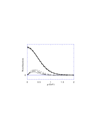
FIG. 14.: Dirac positive ground state solutions for three values of the vector strength $y$: $y=0.0$, $E_{1}$=0.976 GeV (circles and squares); $y=0.4$, $E_{1}$=1.028 GeV (solid and long dashed lines); and for $y=0.6$, $E_{1}$=1.065 GeV (heavy short dashed and dotted lines).

FIG. 15.: Dirac positive first excited state solutions for $y=0.0$, $E_{2}=1.394$ GeV (circles and squares), for $y=0.4$, $E_{2}$=1.456 GeV (solid and long dashed lines), and for $y=0.6$, $E_{2}$=1.496 GeV (heavy short dashed and dotted lines).

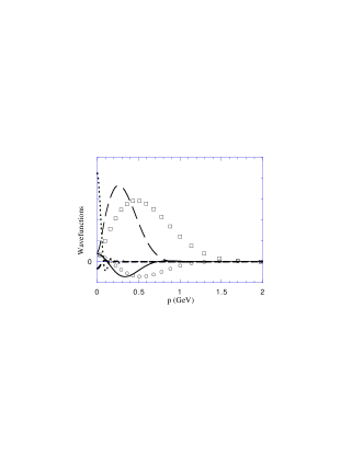
FIG. 16.: Dirac negative ground state solutions for $y=0.0$, $E_{-1}=-1.249$ GeV (circles and squares), for $y=0.4$, $E_{-1}$=-0.660 GeV (solid and long dashed lines), and for $y=0.6$, $E_{-1}=2.028$ GeV (heavy short dasheded and dotted lines).

The Dirac wave functions are shown in Figs. 14–16. Fig. 14 gives the positive energy ground states, Fig. 15 the first positive energy excited states, and Fig. 16 the negative energy ground states. By comparing the solutions for the states with $y<1/2$ (which are known to be stable) with the $y=0.6$ solutions, we conclude that (i) the positive energy $y=0.6$ state has a structure identical to the other positive energy states, and hence appears to be stable (as already suggested by the stability of the eigenvalue shown in Table IV), but (ii) the negative energy $y=0.6$ ground state, shown in Fig. 16, has a radically different structure (similar to a momentum space delta function) showing that it is indeed unstable. All of the $y=1.0$ solutions (not shown in the figures) have a behavior similar to the negative energy $y=0.6$ solution, confirming that they are unstable.

The apparant stability of the $y=0.6$ positive energy solution differs from expectations based on the discussion in Sec. II and examination of Fig. 8. We expect all positive energy solutions for $y>1/2$ to be unstable, but as Fig. 8 shows, the positive and negative energy surfaces actually overlap in the $y=1.0$ case but remain clearly separated for the $y=0.6$ case. This suggests that the instability of the $y=0.6$ positive energy state is hard to observe numerically because the distance between the positive and negative energy surfaces is large and the “leakage” from positive to negative energy is very small (also suggested by Fig. 4). Presumably a more precise numerical calculation would uncover some instability in the positive energy $y=0.6$ case, but this further calculation is not needed because the overlap of the positive and negative energy spectrum (condition 3) is already a sign of the instability.

We conclude that the fourth stability condition largely reinforces the conclusions we have already drawn, but that it should be used in conjunction with the other three. The stability of a single state cannot easily be determined solely by tracking (with changing spline number) its behavior. A reliable conclusion requires the examination of the entire spectrum, with particular attention to condition 3.

B The one-channel spectator equation

As in the Dirac case the antiquark mass will be set to $m_{2}=0.325$ GeV and the confinement strength to $\sigma=0.2$ GeV². We will present results for heavy quark masses $m_{1}=\kappa\,m_{2}$ with the mass ratio $\kappa=10$, 5, 2, and 1. In order to compare the 1CS results to those obtained from the Dirac equation, we define an effective Dirac-like binding energy $E_{D}$ using the relation

$$\mu=E_{D}+m_{1}\,$$ (120)

where $\mu$ is the mass eigenvalue obtained from the 1CS equation. This relation insures that the effective 1CS binding energy must approach the Dirac binding energy as $m_{1}\to\infty$. Tables V and VI give these effective binding energies (instead of the bound state masses).

TABLE V.: First four positive and negative energy levels for the 1CS equation for mass ratios $\kappa$=5.0 and 10.0 and vector strength $y$=0.0 and 0.4. Here $E_{D}$ is shown in GeV and solutions for spline ranks of 20 and 12 are compared.

	$y=0.0\;$ $\kappa=5.0$		$y=0.0\;$ $\kappa=10.0$		$y=0.4\;$ $\kappa=5.0$		$y=0.4\;$ $\kappa=10.0$
Level	SN=20	SN=12	SN=20	SN=12	SN=20	SN=12	SN=20	SN12
4	2.109	2.113	2.073	2.078	2.225	2.227	2.165	2.168
3	1.808	1.808	1.783	1.783	1.898	1.899	1.858	1.858
2	1.443	1.443	1.435	1.435	1.509	1.509	1.495	1.494
1	0.940	0.939	0.964	0.964	0.992	0.992	1.013	1.013
-1	-0.936	-0.936	-1.091	-1.090	-0.548	-0.569	-0.619	-0.619
-2	-1.084	-1.084	-1.333	-1.332	-0.570	-0.607	-0.715	-0.715
-3	-1.173	-1.170	-1.511	-1.515	-0.600	-0.637	-0.786	-0.785
-4	-1.233	-1.259	-1.650	-1.642	-0.630	-0.675	-0.841	-0.848

Note that results for the equal mass ($\kappa=1.0$) 1CS equation are included only for comparison because the 1CS equation should not be used for equal mass systems. If the equal mass particles are identical (as in $NN$ scattering) the equation must be symmetrized in order to preserve the Pauli principle. Even if the equal mass particles are not identical, as for the $q\bar{q}$ pairs discussed in this paper, the equation must still be symmetrized to insure charge conjugation invariance. Furthermore, for bound states with a very small mass (e.g., the pion) the symmetrized two channel spectator equation defined in Ref. [12] should be used.

TABLE VI.: First four positive and negative energy levels for the 1CS equation for the mass ratio $\kappa$=1.0 and vector strength $y$=0.0 and 0.4. Here $E_{D}$ is shown in GeV and solutions for spline ranks of 24, 20, 16, and 12 are compared.

	$y=0.0$				$y=0.4$
Level	SN=24	SN=20	SN=16	SN=12	SN=24	SN=20	SN=16	SN12
4	1.881	1.881	1.881	1.881	2.222	2.222	2.222	2.223
3	1.630	1.630	1.630	1.632	1.884	1.884	1.884	1.884
2	1.294	1.293	1.293	1.293	1.461	1.461	1.461	1.461
1	0.745	0.745	0.745	0.745	0.853	0.853	0.853	0.853
-1	-0.329	-0.330	-0.331	-0.334	0.933	0.724	0.508	0.284
-2	-0.331	-0.332	-0.335	-0.341	0.727	0.527	0.326	0.122
-3	-0.334	-0.337	-0.342	-0.354	0.577	0.387	0.196	0.005
-4	-0.338	-0.343	-0.353	-0.379	0.454	0.272	0.091	-0.087

The eigenvalues are real for all values of the vector strength $y$ and the mass ratio $\kappa$ (condition 1). However only systems with a vector strength less than 1/2 (0.0 and 0.4) have stable eigenvalues (condition 2). Cases which fail the first two stability conditions ($y=0.6$ and 1.0) are not listed in the eigenvalue tables. Table V shows the eigenvalues for mass ratios $\kappa$=5.0 and 10.0. These cases are very similar to the Dirac cases, and the table shows that in all cases the spectra satisfy condition 3 (no overlap of the positive and negative energy sectors). Table VI shows the eigenvalues for the equal mass case ($\kappa$=1.0). Note that condition 3 is violated for $y$=0.4; at a spline rank of 24 the negative energy state (shown in bold face) crosses into the positive energy sector. In the equal mass case only the pure scalar interaction is stable. The binding energies for $\kappa=2.0$ (not shown in the tables) exhibit the same behavior as for $\kappa=1.0$.

FIG. 17.: Positive ground state soutions for the quasirelativistic 1CS equation with a pure scalar interaction. The solid and long dashed lines are for $\kappa$=5.0, $E_{1}$=0.940 GeV; the heavy short dashed and dotted lines are for $\kappa$=10.0, $E_{1}$=0.964 GeV. The scalar ground state Dirac solution for $E_{1}=0.976$ GeV is shown for comparison (circles and squares).

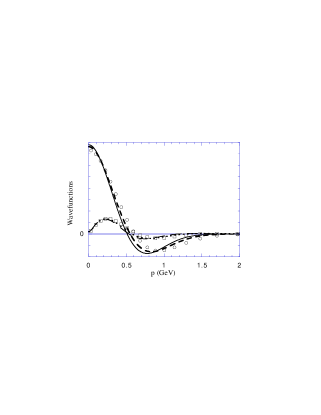
FIG. 18.: Positive first excited state solutions labeled as in Fig 17. Here the $\kappa=5.0$ solution has an energy of $E_{2}=1.443$ GeV and the $\kappa=10.0$ solution an energy of $E_{2}=1.435$ GeV compared to the Dirac energy of $E_{2}=1.394$ GeV.

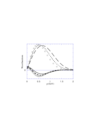
FIG. 19.: Negative ground state soutions labeled as in Fig 17. Here the $\kappa=5.0$ solution has an energy of $E_{-1}=-0.936$ GeV and the $\kappa=10.0$ solution an energy of $E_{-1}=-1.091$ GeV compared to the Dirac energy of $E_{-1}=-1.249$ GeV.

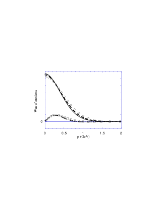
FIG. 20.: Positive ground state solutions of the quasirelativistic 1CS equation with a mixed scalar and vector interaction ($y=0.4$) for two mass ratios $\kappa$. The solid and long dashed lines are for $\kappa=5.0$, $E_{1}=0.992$ GeV, and the heavy short dashed and dotted lines are for $\kappa=10.0$, $E_{1}=1.013$ GeV. The circles and squares show the solution for the Dirac equation with $E_{1}=1.028$ GeV.

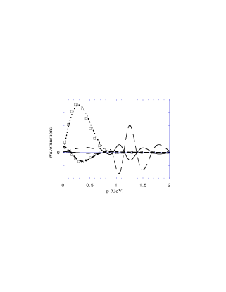
FIG. 21.: Negative ground state solutions of the quasirelativistic 1CS equation for $y=0.4$ labeled as in previous figure. Here $\kappa=5.0$, $E_{-1}=-0.548$ GeV and $\kappa=10.0$, $E_{-1}=-0.619$ GeV. The comparison Dirac level has energy $E_{-1}=0.660$ GeV.

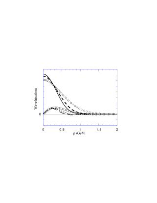
FIG. 22.: Positive ground state soutions for the quasirelativistic 1CS equation with a pure scalar interaction. The solid and long dashed lines are for $\kappa$=1.0, $E_{1}$=0.745 GeV; the heavy short dashed and dotted lines are for $\kappa$=2.0, $E_{1}$=0.857 GeV. The scalar ground state Dirac solution for $E_{1}=0.976$ GeV is shown for comparison (circles and squares).

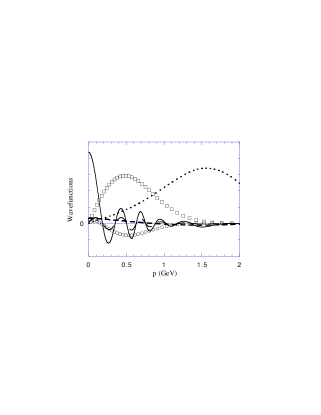
FIG. 23.: Negative ground state solutions labeled as in previous figure. Here the $\kappa=1.0$ solution has an energy of $E_{-1}=-0.330$ GeV and the $\kappa=2.0$ solution an energy of $E_{-1}=-0.607$ GeV compared to the Dirac energy of $E_{-1}=-1.249$ GeV.

Wave functions for the 1CS equation are shown in Figs. 17–23. In Figs. 17–19 the wave functions for a large mass ratio and a pure scalar confinement are compared with the Dirac solutions. Both the positive and negative states for these systems are completely stable and very similar to the corresponding Dirac solutions. We also observe how the 1CS binding energies approach the Dirac values as $\kappa$ is increased.

Figs. 20 and 21 show the wave functions for large mass ratios and a vector strength of 0.4. For $\kappa$=10.0 the system is once again totally stable, while for $\kappa$=5.0 only the positive states are stable. In this case the instability of the negative energy states is not accompanied by violation of condition 3; the only indication of instability is the variation of the negative energy levels with spline rank (condition 2), as shown in Table V. In this case the structure (condition 4) reinforces condition 2, and we have a first example of a system where the positive energy solutions are stable and the negative energy ones are not.

The positive and negative ground states for $\kappa=1.0$ and 2.0 are shown in Figs. 22 and 23. Note that the positive energy states are stable while the negative energy ones are not. Here the instability of the negative energy states is only apparant from an examination of the structure of the wave functions; neither condition 2 (variation of the energy with spline rank) nor condition 3 (penetration of the positive energy sector) seems to occur.

In conclusion, the 1CS system becomes more stable as the vector strength is decreased and the mass of the heavy quark is increased. This will be summarized further at the end of this section.

C The Salpeter Equation

The use of pure scalar confinement with the Salpeter equation gives the first example of instability due to the mass eigenvalues becoming complex (condition 1). Actually, the eigenvalues become pure imaginary because the mass squared is real and negative. This situation is accompanied by a very rapid variation of $\mu^{2}$ with spline rank, as shown in Table VII. However, for $y$=0.4 the tabulated spectra do not vary with the spline rank, and these states are stable, as shown in Figs. 24–26. Fig. 24 also shows that the wave functions for positive and negative energies are identical provided $\psi_{1a}\leftrightarrow\psi_{2a}$. This is a further consequence of the symmetry of the Salpeter equation which produces pairs of eigenvalues with the same magnitude and opposite signs.

TABLE VII.: Square of the mass ($\mu^{2}$ in GeV²) of the first four levels of the Salpeter equation for $y$=0.0 and 0.4 with various spline ranks.

	$y=0.0$		$y=0.4$
Level	SN=20	SN=12	SN=20	SN=16	SN=12
4	0.685	2.173	5.632	5.632	5.674
3	-1.074	1.538	4.383	4.383	4.385
2	-3.869	0.931	2.977	2.977	2.976
1	-8.705	-0.051	1.339	1.339	1.339

The two figures, Fig. 24 (ground state) and Fig. 25 (second excited state), demonstrate that these Salpeter systems have solutions comparable to their Dirac counterparts. In addition, Fig. 26 illustrates that the $y$=0.6 and 1.0 solutions are indeed stable by showing that they have the correct structure with the right number of nodes for a second excited state.

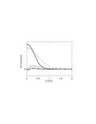
FIG. 24.: Positive and negative ground state solutions for the $y=0.4$ quasirelativistic equal mass Salpeter equation, $\mu_{1}$=1.157 GeV (solid and long dashed lines) and $\mu_{-1}$=-1.157 GeV (heavy short dashed and dotted lines). The positive ground state Dirac solutions for $y$=0.4, $E_{1}$=1.028 GeV (circles and squares) are shown for comparison.

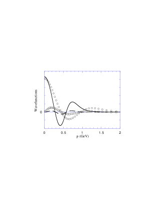
FIG. 25.: The positive second excited state solutions for the $y$=0.4 equal mass Salpeter equation, $\mu_{3}=2.094$ GeV (solid and long dashed lines) are compared to the second positive excited state Dirac solution for $y=0.4$, $E_{3}$=1.772 GeV (circles and squares).

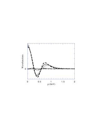
FIG. 26.: Positive second excited state solutions for the Salpeter equation for a variety of scalar/vector mixings: pure vector $y$=1.0, $\mu_{3}$=2.565 GeV (circles and squares); $y$=0.6, $\mu_{3}$=2.284 GeV (solid and long dashed lines); and $y$=0.4 $\mu_{3}$=2.094 GeV (heavy short dashed and dotted lines).

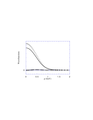
FIG. 27.: Stable ground state solution for the Salpeter equation with a pure scalar confining interaction. In these cases $m=0.85$ GeV and the Salpeter bound state has mass $\mu_{1}$=2.185 GeV. The solutions for SN=20 (circles and squares) and SN=30 (solid and long dashed lines) are compared. (Note that the solutions are not normalized – see the discussion in the text.)

While it is true that the scalar Salpeter equation is unstable for equal quark-antiquark masses of 0.325 GeV, increasing the mass of the quarks will give stable solutions (this was anticipated by the discussion in Sec. III). We find that the lower mass states of the $y$=0.0 Salpeter equation are stable when the quark mass is increased to $m$=0.85. The ground state wave functions for this case are shown in Fig. 27, where solutions for spline ranks of 20 and 30 are compared (since the wave functions have not been normalized, only the shape of the two solutions should be compared). Solutions obtained for somewhat lower masses (m=0.65, for example) appear stable for SN=20, but the spectrum shows some instability for SN=30. In general, the number of stable states for the pure scalar Salpeter equation increases as the quark mass increases. Further study is needed to obtain a detailed understanding of the stability of the purely scalar Salpeter equation.

TABLE VIII.: Stability Results (the table lists the region of stability or the first of the four tests that the system fails).

	$y=0.0$	$y=0.4$	$y=0.6$	$y=1.0$
Dirac	stable	stable	Cond 2	Cond 2
1CS $\kappa$=1.0	positive	Cond 3	Cond 2	Cond 2
1CS $\kappa$=2.0	positive	Cond 3	Cond 2	Cond 2
1CS $\kappa$=5.0	stable	positive	Cond 2	Cond 2
1CS $\kappa$=10.0	stable	stable	Cond 2	Cond 2
Salpeter	m$\geq$ 0.85 GeV	stable	stable	stable

V Conclusions

Table VIII summarizes the results presented in the previous sections, which are also outlined below:

• The Dirac equation is stable if the scalar confinement is stronger than the vector confinement ($y<1/2$).

• The Salpeter equation is stable if the interaction is mostly vector, and perhaps also for pure scalar exchanges with a large quark mass. The precise boundary between stable and unstable solutions is presumably a function of the quark mass $m$ and the vector strength $y$, and we have not mapped it out.

• The one channel spectator (1CS) equation has the Dirac limit, as expected. This means that for large mass ratios $\kappa=m_{1}/m_{2}$, it is stable if the interaction is predominately scalar ($y<1/2$). However, as the mass ratio decreases toward unity, the region of instability grows. As we decrease $\kappa$ for a fixed vector strength $y<1/2$, the negative energy states will first become unstable, and then the positive energy states may follow. However, if the vector strength is small enough (e.g., $y=0$) the positive energy states appear to be stable for all mass ratios.

The usefulness of an equation where only part if the spectrum is stable depends on whether or not the spectrum of unstable states is clearly separate from the spectrum of stable states (i.e. Condition 3 is met). The 1CS equation for scalar confinement has this feature; the unstable states are those which map, in the Dirac limit, into negative energy states. If one is content to exclude these states from consideration on physical grounds then the scalar 1CS equation can be used to describe confined $Q\bar{q}$ systems for all mass ratios. The Salpeter equation can also be used for equal mass $q\bar{q}$ systems unless the confinement is predominately scalar and the quark masses are not large.

This conclusion answers one of the questions raised in the introduction; clearly the stability of vector or scalar confinement depends on the relativistic equation used. Scalar confinement is stable if the 1CS equation is used and vector confinement is stable if the Salpeter equation is used.

We emphasize that our study of the stability of the spectator equation is preliminary for three reasons:

• Only the 1CS equation has been studied. As emphasized before, a two channel spectator equation must be used if the bound state mass is small (the pion), and any spectator equation must be explicitly symmetrized if the quark masses are equal.

• Our study of the 1CS equation was limited to the quasirelativistic approximation, in which retardation is neglected. However, neglecting retardation usually leads directly to the Salpeter equation, and the attempt to include it (at least approximately) is the principle reason for choosing to use a spectator equation in the first place. Including retardation in our analysis (planned for a later work) may alter our conclusions.

• Only the time-like part of a vector confinement (i.e. $\gamma^{0}\gamma^{0}$) has been studied. There are preliminary indications that our results will change when the full vector interaction $\gamma^{\mu}\gamma_{\mu}$ is included.

Our results for the Salpeter equation agree with Ref. [4], but disagree with the results obtained by Parramore and Piekarewicz [3], who found the Salpeter equation to be unstable once the vector strength dropped below one-half, regardless of quark mass. However, as stated above, we find that the Salpeter equation is stable for a vector strength 0.4, and is even stable for a pure scalar interaction provided the quark mass is sufficiently large. We looked at one of the cases they found to be unstable ($\sigma$=0.29, $m$=0.9 GeV, with 25 basis states), and found it to contain stable states. A possible explanation for this difference is that we use cubic splines for our basis functions, while nonrelativistic harmonic oscillator wave functions were used in Ref. [3].

There are other equations which can be used to model the quark-antiquark system. Tiemeijer and Tjon [13] explored two such equations, the Blankenbecler-Sugar-Logunov-Tavkhelidze (BSLT)[14] equation and the equal-time (ET) equation of Wallace and Mandelzweig[15]. The kernels for both equations contained one-gluon-exchange (with the full four vector structure) and a linear confining term (with a mixed scalar-four vector structure). They found that increasing the vector strength of the confining term improved the phenomenology, but that some mesons became unstable for vector strengths of more than about 0.25, depending on the equation and gauge used. These results reinforce the general conclusions of this paper: stability depends on both the Lorentz structure of confinement and on the type of relativistic equation used.

We have seen that the study of the mathematical stability of relativistic equations requires the examination of both local and global features of the eigenvalue spectrum and have introduced four conditions which must be satisfied for an equation to give stable solutions. Using these stability criteria we find that the Lorentz structure of the kernel and the equation used to model the meson both play a crucial role in the mathematical stability of the system. Clearly further research on this topic is needed.

A Spline functions and numerical methods

To solve the equations in this paper numerically, we expand each momentum space wave function in terms of cubic splines

$$\psi_{i}(p)=\sum_{j=1}^{{\rm SN}}\alpha^{i}_{j}\beta_{j}(p)\,,$$ (A1)

where $\alpha^{i}_{j}$ are the expansion coefficients (which become the eignevectors of the problem), $\beta_{j}$ are the spline functions, and SN is the number of spline functions in the expansion (the spline rank). In all of the equations studied there are only two independent wave functions, so $i=$ 1 or 2. Since the angular integrations are performed analytically, the wave functions depend only on the magnitude of the momentum $p$. Once Eq. (A1) is substituted for each of the wave functions, both sides of the equation are operated on by the integral operator

$$\int p^{2}\beta_{l}(p)dp\,.$$ (A2)

This reduces the integral equations to matrix equations with dimension 2SN$\times$2SN and of the general form

$$\left\{\lambda\pmatrix{A_{lj}&0\cr 0&A_{lj}}+\pmatrix{B^{11}_{lj}&0\cr 0&B^{22}_{lj}}-\pmatrix{V^{11}_{lj}&V^{12}_{lj}\cr V^{21}_{lj}&V^{22}_{lj}}\right\}\pmatrix{\alpha^{1}_{j}\cr\alpha^{2}_{j}}=0\,.$$ (A3)

These equations are then solved for the eigenvalues $\lambda$ and the eigenvectors $\{\alpha^{1}_{j},\;\alpha^{2}_{j}\}$. In the following subsections we give the forms of the matrices $A$ and $V$ for each case studied in this paper.

1 Dirac equation

The Dirac equation was given in Eq. (77) and (39). The two independent wave functions are

$$\psi_{1}= \psi_{1a}$$ (A4)

$$\psi_{2}= \psi_{1b}\,,$$ (A5)

and $\lambda=E_{B}$,

$$A_{lj}=\int_{0}^{\infty}p^{2}dp\;\beta_{l}(p)\beta_{j}(p)\,,$$ (A6)

and

$$B^{11}_{lj}=-B^{22}_{lj}=-\int_{0}^{\infty}p^{2}dp\;E_{p}\,\beta_{l}(p)\beta_{j}(p)\,.$$ (A7)

Setting $m_{2}=m$ and using the notation

$$f_{l}(p)=\frac{N_{p}}{\sqrt{2E_{p}}}\;\beta_{l}(p)\,,$$ (A8)

the potential matrix can be written

$$\pmatrix{V^{11}_{lj}&V^{12}_{lj}\cr V^{21}_{lj}&V^{22}_{lj}}=$$ (A9)

$$\qquad-\frac{4\sigma}{\pi}\int_{0}^{\infty}\int_{0}^{\infty}dp\,dk\;V_{0}(p,k)\,f_{l}(p)\left\{f_{j}(k)\pmatrix{\eta_{1}&\eta_{2}\cr\eta_{3}&\eta_{4}}-f_{j}(p)\pmatrix{\eta^{\prime}_{1}&\eta^{\prime}_{2}\cr\eta^{\prime}_{3}&\eta^{\prime}_{4}}\right\}$$ (A10)

$$\qquad-\frac{4\sigma}{\pi}\int_{0}^{\infty}\int_{0}^{\infty}dp\,dk\;V_{1}(p,k)\,f_{l}(p)f_{j}(k)\pmatrix{\zeta_{5}&\zeta_{6}\cr\zeta_{7}&\zeta_{8}}\,.$$ (A11)

The functions $\eta$ and $\zeta$ are

$$\eta_{i}=a_{i}+b_{i}\qquad\zeta_{i}=b_{i}$$ (A12)

where $a_{i}$ and $b_{i}$ were defined in Eq. (78), and if $\eta_{i}=\eta_{i}(p,k)$, then $\eta^{\prime}_{i}=\eta_{i}(p,p)$. The functions $V_{0}$ and $V_{1}$ are

$$V_{0}(p,k)=\frac{1}{2}\int_{-1}^{1}dz\frac{p^{2}k^{2}}{(p^{2}+k^{2}-2pkz)^{2}}= \frac{p^{2}k^{2}}{(p^{2}+k^{2})^{2}-4p^{2}k^{2}}$$ (A13)

$$V_{1}(p,k)=\frac{1}{2}\int_{-1}^{1}dz\frac{p^{2}k^{2}\,(z-1)}{(p^{2}+k^{2}-2pkz)^{2}}= \frac{1}{2}\frac{pk}{(p^{2}+k^{2}+2pk)}$$ (A15)

$$-\frac{1}{8}\log\left(\frac{p^{2}+k^{2}+2pk}{p^{2}+k^{2}-2pk}\right)\,.$$

2 One-channel spectator equation

The 1CS equation in helicity form was given in Eq. (71) with the potential defined in Eq. (42) [with $(p-k)^{2}\to({\bf p}-{\bf k})^{2}$ as discussed in Sec. IIB]. The two independent wave functions are as in Eq. (A5) and $\lambda=\mu=m_{1}+E_{B}$. The matrix $A$ is identical to the Dirac case, but now

$$B^{11}_{lj} =-\int_{0}^{\infty}p^{2}dp\;\left(E_{p_{1}}+E_{p_{2}}\right)\,\beta_{l}(p)\beta_{j}(p)$$ (A16)

$$B^{22}_{lj} =-\int_{0}^{\infty}p^{2}dp\;\left(E_{p_{1}}-E_{p_{2}}\right)\,\beta_{l}(p)\beta_{j}(p)\,.$$ (A17)

Introducing the notation

$$F_{l}(p)=\frac{N_{p_{1}}N_{p_{2}}}{\sqrt{4E_{p_{1}}E_{p_{2}}}}\;\beta_{l}(p)\,,$$ (A18)

the potential matrix can be written

$$\pmatrix{V^{11}_{lj}&V^{12}_{lj}\cr V^{21}_{lj}&V^{22}_{lj}}=$$ (A19)

$$\qquad-\frac{4\sigma}{\pi}\int_{0}^{\infty}\int_{0}^{\infty}dp\,dk\;V_{0}(p,k)\,F_{l}(p)\left\{F_{j}(k)\pmatrix{\overline{\eta}_{1}&\overline{\eta}_{2}\cr\overline{\eta}_{3}&\overline{\eta}_{4}}-\frac{E_{p_{1}}}{E_{k_{1}}}F_{j}(p)\pmatrix{\overline{\eta}^{\prime}_{1}&\overline{\eta}^{\prime}_{2}\cr\overline{\eta}^{\prime}_{3}&\overline{\eta}^{\prime}_{4}}\right\}$$ (A20)

$$\qquad-\frac{4\sigma}{\pi}\int_{0}^{\infty}\int_{0}^{\infty}dp\,dk\;V_{1}(p,k)\,F_{l}(p)F_{j}(k)\pmatrix{\overline{\zeta}_{1}&\overline{\zeta}_{2}\cr\overline{\zeta}_{3}&\overline{\zeta}_{4}}\,,$$ (A21)

with

$$\overline{\eta}_{i}=A_{i}+B_{i}\qquad\overline{\zeta}_{i}=B_{i}\,,$$ (A22)

where the $A_{i}$ and $B_{i}$ were defined in Eq. (76). The meaning of the prime in $\overline{\eta}^{\prime}$ is the same as in $\eta^{\prime}$ and $V_{0}$ and $V_{1}$ are as before.

3 Salpeter equation

The Salpeter equation is given in Eq. (81), with the masses both equal to $m$. Now

$$\psi_{1}= \psi_{1a}$$ (A23)

$$\psi_{2}= \psi_{2a}\,,$$ (A24)

and $\lambda=\mu$. The matrix $A$ is identical, but $B$ is two times the Dirac $B$. The potential matrix is similar to Eq. (A21) with

$$\begin{array}[]{ll}\overline{\eta}_{2}\to\eta_{5}&\overline{\zeta}_{2}\to\zeta_{5}\cr\overline{\eta}_{3}\to-\eta_{5}&\overline{\zeta}_{3}\to-\zeta_{5}\cr\overline{\eta}_{4}\to-\overline{\eta}_{1}&\overline{\zeta}_{4}\to-\overline{\zeta}_{1}\,,\end{array}$$ (A25)

and, from Eq. (82),

$$\eta_{5}=\tilde{p}^{2}+\tilde{k}^{2}+2(1-2y)\tilde{p}\tilde{k}\qquad\zeta_{5}=2(1-2y)\tilde{p}\tilde{k}\,.$$ (A26)

4 Splines

The solution to the wavefunctions used in this paper are based on a set of third order polynomial functions called cubic splines. Used previously in papers such as Ref. [10], they have proven versatile enough to model all of the wavefunctions examined in this paper.

The wave function expansion was given in Eq. (A1). Each spline is constucted from four separate functions. The function used depends on the argument and the spline index $j$ as shown:

$$4\beta_{j}(x)=\left\{\begin{array}[]{ll}\frac{(x-x_{j-2})^{3}}{h^{3}}\,,&x\in[x_{j-2},x_{j-1}]\\ 1+3\frac{(x-x_{j-1})}{h}+3\frac{(x-x_{j-1})^{2}}{h^{2}}-3\frac{(x-x_{j-1})^{3}}{h^{3}}\,,&x\in[x_{j-1},x_{j}]\\ 1+3\frac{(x_{j+1}-x)}{h}+3\frac{(x_{j+1}-x)^{2}}{h^{2}}-3\frac{(x_{j+1}-x)^{3}}{h^{3}}\,,&x\in[x_{j},x_{j+1}]\\ \frac{(x_{j+2}-x)^{3}}{h^{3}}\,,&x\in[x_{j+1},x_{j+2}]\\ 0&{\rm otherwise}\,.\\ \end{array}\right.$$ (A27)

Each spline is defined on the interval from zero to one. This range is divided into sectors whose size, $h=1/({\rm SN}+1)$, depends on the spline rank. Each sector is bounded by nodes at $x_{k}$ and $x_{k+1}$, with the number of nodes equal to SN$+2$. The first node, $x_{1}$, is always located at zero, and the last one, $x_{{\rm SN}+2}$, at one. The spline curves for a spline rank of 4 are given in Fig. 28. The standard choice for our calculation was a rank of 20 (20 splines in each wave function expansion).

None of the nodes may lie outside of the interval from 0 to 1, so the first spline, $j=1$, is defined entirely by the third and forth functions given in Eq. (A27). It has a zero slope at $x=0$. The $j=2$ spline was defined in a special way so that it too will have zero slope at $x=0$ (insuring that all the splines have this property). To accomplish this the first sector (which lies between $x_{0}$ and $x_{1}$ and is hence outside the acceptable range of support) will be “folded over” onto the interval between $[x_{1},x_{2}]$. Hence, in the interval between $[x_{1},x_{2}]$ the second spline is defined to be

$$4\beta_{2}(x)=1+3\frac{(x-x_{1})}{h}+3\frac{(x-x_{1})^{2}}{h^{2}}-3\frac{(x-x_{1})^{3}}{h^{3}}+\frac{(x_{2}-x)^{3}}{h^{3}}\,.$$ (A28)

This is an exceptional case, and all other splines are defined following Eq. (A27) in a straightforward fashion.

FIG. 28.: Spline rank 4 curves (1 solid, 2 long dashed, 3 short dashed, and 4 dotted).

FIG. 29.: Spline rank 4 curves (1 solid, 2 long dashed, 3 short dashed, and 4 dotted) with momentum arguement.

The splines defined in Eq. (A27) are only continuous up to their second derivative. Therefore, in order to obtain convergence the integrals must be separately evaluated for each sector, and the results from all the sectors summed up afterwards. Special care must be taken in evaluating those contributions to the double integral of the potential which include singularities. These are evaluated by choosing points equally spaced on each side of the singularity so that a well defined limit is obtained.

To use the splines to describe the wave functions, the interval $[0,\infty)$ is mapped into the line segment $[0,1]$ using the tangent mapping

$$x=\frac{2}{\pi}\arctan\left(\frac{p}{\Lambda}\right)\,,$$ (A29)

with $\Lambda=1$ GeV. This mapping alters the shape of the splines, as illustrated in Fig. 29.

When the spline rank is increased the sectors become smaller and the range in momentum space over which the splines are significantly different from zero increases. Thus, the wave function is more accurately modeled as the spline rank increases. Of course this higher precision must be balanced by consideration of computation time.

REFERENCES

- [1] D. Gromes, Institut für Theoretische Physik, Fed. Rep. Germany. Nov. 3, 1987.
- [2] J. L. Lagaë, Service de Physique Théorique, Université Libre de Bruxelles, Belgium, Jan. 26, 1990.
- [3] J. Parramore and J. Piekarewicz, Nucl. Phys. A 585, 705 (1995).
- [4] J. Resag, C. R. Münz, B. C. Metsch, and H. R. Petry, Nucl.. Phys. A578, 397 (1994); C. R. Münz, J. Resag, B. C. Metsch, and H. R. Petry, Nucl. Phys. A578, 418 (1994).
- [5] J. D. Bjorken and S. D. Drell, Relativistic Quantum Mechanics (McGraw-Hill Inc., New York, 1964).
- [6] E. E. Salpeter and H. A. Bethe, Phys. Rev. 84, 1232 (1951).
- [7] F. Gross, Relativistic Quantum Mechanics and Field Theory (John Wiley and Sons Inc., New York, 1993).
- [8] F. Gross, J. W. Van Orden, and K. Holinde, Phys. Rev. C 45, 2094 (1992).
- [9] F. Gross and J. Milana, Phys. Rev. D 43, 2401 (1991).
- [10] F. Gross and J. Milana, Phys. Rev. D 50, 3332 (1994).
- [11] E. E. Salpeter, Phys. Rev. 87, 328 (1952).
- [12] F. Gross, Phys. Rev. 186, 1448 (1969).
- [13] P. Tiemeijer and J. A. Tjon, Phys. Rev. C 49, 494 (1994).
- [14] R. Blankenbecler and R. Sugar, Phys. Rev. 142, 1051 (1966); A. A. Logunov and A. N. Tavkhelidze, Nuovo Cimento 29, 380 (1963).
- [15] S. J. Wallace and V. B. Mandelzweig, Nucl. Phys. A503, 673 (1989).
- [16] M. Ortalano, et. al. unpublished.