Center for Nuclear Studies, Physics Department, The George Washington University, Washington, DC 20052, U. S. A. and Jurusan Fisika, FMIPA, Universitas Indonesia, Depok 16424, Indonesia and Institut für Theoretische Physik, Universität Gießen, D-35392 Gießen, Germany

Kaon Photoproduction with Form Factors in a Gauge-invariant Approach

Abstract

The general gauge-invariant photoproduction formalism given by Haberzettl is applied to kaon photoproduction off the nucleon at the tree level, with form factors describing composite nucleons. We demonstrate that, in contrast to Ohta’s gauge-invariance prescription, this formalism allows electric current contributions to be multiplied by a form factor, i.e., they do not need to be treated like bare currents. Numerical results show that Haberzettl’s gauge procedure, when compared to Ohta’s, leads to much improved $\chi^{2}$ values. Moreover, predictions for the new Bonn SAPHIR data for $p(\gamma,K^{+})\Lambda$ are given.

Gauge invariance is one of the central issues in dynamical descriptions of how photons interact with hadronic systems (see Ref. [1], and references therein). For the simple example of $\gamma p\rightarrow n\pi^{+}$ with pseudoscalar coupling for the $\pi NN$ vertex, one finds already at the tree level (see Fig. 1) that the corresponding amplitude violates gauge invariance if the baryon structure is described by form factors. This amplitude may be written as [2]

$$\epsilon\cdot\widetilde{M}_{fi}=\sum_{j=1}^{4}\widehat{A}_{j}\overline{u}_{n}\left(\epsilon_{\mu}M_{j}^{\mu}\right)u_{\rm p}-2ge\overline{u}_{\text{n}}\gamma_{5}\epsilon_{\mu}\bigg{[}p^{\prime\mu}\frac{\widehat{F}-F_{s}}{s-m^{2}}+q^{\mu}\frac{\widehat{F}-F_{t}}{t-\mu^{2}}\bigg{]}u_{\text{p}}\;\;,$$ (1)

with individually gauge-invariant currents,

$$M_{1}^{\mu} = -\gamma_{5}\gamma^{\mu}\;k\cdot\gamma\;\;,$$ (2)

$$M_{2}^{\mu} = 2\gamma_{5}\left(p^{\mu}\;k\cdot p^{\prime}-p^{\prime\mu}k\cdot p\;\right)\;\;,$$ (3)

$$M_{3}^{\mu} = \gamma_{5}\left(\gamma^{\mu}\;k\cdot p-p^{\mu}\;k\cdot\gamma\right)\;\;,$$ (4)

$$M_{4}^{\mu} = \gamma_{5}\left(\gamma^{\mu}\;k\cdot p^{\prime}-p^{\prime\mu}\;k\cdot\gamma\right)\;\;,$$ (5)

with coefficient functions

$$\widehat{A}_{1} = \frac{ge}{s-m^{2}}\left(1+\kappa_{\rm p}\right)F_{s}+\frac{ge}{u-m^{2}}\kappa_{n}F_{u}\;\;,$$ (6)

$$\widehat{A}_{2} = \frac{2ge}{(s-m^{2})(t-\mu^{2})}\widehat{F}\;\;,$$ (7)

$$\widehat{A}_{3} = \frac{ge}{s-m^{2}}\frac{\kappa_{p}}{m}F_{s}\;\;,$$ (8)

$$\widehat{A}_{4} = \frac{ge}{u-m^{2}}\frac{\kappa_{n}}{m}F_{u}\;\;,$$ (9)

and a gauge-violating term given by the last term in Eq. (1).

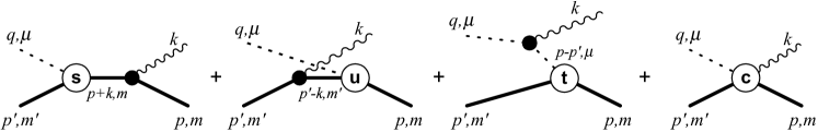
Figure 1: Tree-level photoproduction diagrams. Time proceeds from right to left. The form factors $F_{s}$, $F_{u}$, and $F_{t}$ in the text describe the vertices labeled $s$, $u$, and $t$, respectively, with appropriate momenta and masses shown for their legs. The right-most diagram corresponds to the contact current $M_{\text{c}}^{\mu}$ required to restore gauge invariance.

With all external legs on-shell in Fig. 1, the respective form factors are only functions of one of the Mandelstam variables, $s$, $u$, or $t$, i.e.,

$$F_{s} = F_{s}(s)\;=\;f\!\left((p+k)^{2},m^{\prime 2},\mu^{2}\right)\;\;,$$ (10)

$$F_{u} = F_{u}(u)\;=\;f\!\left(m^{2},(p^{\prime}-k)^{2},\mu^{2}\right)\;\;,$$ (11)

$$F_{t} = F_{t}(t)\;=\;f\!\left(m^{2},m^{\prime 2},(p-p^{\prime})^{2}\right)\;\;,$$ (12)

where $f\!(p^{2},{p^{\prime}}^{2},q^{2})$ is a general $\pi NN$ form factor depending on the squared four-momenta of its three hadronic legs.

The function $\widehat{F}$ appearing here cancels out in Eq. (1), and hence it is undetermined. Introducing this free function here allows us to write Eq. (1) so that the gauge-invariant limit of having no form factors, viz.

$$\text{Point-likenucleons:\quad}F_{s}=F_{u}=F_{t}=\widehat{F}=1\;,$$ (13)

immediately provides for vanishing of the gauge-violating contribution to the amplitude (1).

For extended nucleons, and without a detailed dynamical treatment of the compositeness of nucleons [1], any prescription for restoring gauge invariance amounts to introducing an additional contact current $M_{\rm c}^{\mu}$ (generically depicted by the fourth diagram in Fig. 1), with on-shell matrix elements cancelling exactly the gauge-violating term in Eq. (1). Apart from purely transverse components, for the present example this contact current is essentially given by the term in the square brackets of Eq. (1). Adding this contact contribution to Eq. (1), one then obtains a gauge-invariant amplitude,

$$\epsilon\cdot\widehat{M}_{fi}=\sum_{j=1}^{4}\widehat{A}_{j}\overline{u}_{n}\left(\epsilon_{\mu}M_{j}^{\mu}\right)u_{p}\;\;,$$ (14)

which does depend on $\widehat{F}$ now via $\widehat{A}_{2}$ of Eq. (7). In other words, we may use $\widehat{F}$ to distinguish between different choices for repairing gauge invariance.

One of the most popular prescriptions for restoring gauge invariance is due to Ohta [3]. Using analytic continuation and minimal substitution, Ohta finds that the required $\widehat{F}$ is constant,

$$\mbox{Ohta: \quad}\widehat{F}=f\!\left(m^{2},m^{\prime 2},\mu^{2}\right)=1\;\;,$$ (15)

determined by the normalization condition for the form factor in the unphysical region where all three legs are on-shell. This corresponds precisely to what one obtains for $\widehat{F}$ in the structureless case (13) and therefore the electric term $\widehat{A}_{2}$ of Eq. (7) is treated as in the bare case, thus effectively freezing all degrees of freedom arising from the compositeness of the $\pi NN$ vertex.

The general meson photoproduction theory of Ref. [1] provides another, more flexible, way of choosing $\widehat{F}$. Haberzettl’s formalism allows one to take $\widehat{F}$ as a linear combination of all form factors appearing in the problem, i.e.,

$$\text{Haberzettl:\quad}\widehat{F}=a_{s}F_{s}(s)+a_{u}F_{u}(u)+a_{t}F_{t}(t)\;\;,$$ (16)

where the coefficients are restricted by $a_{s}+a_{u}+a_{t}=1$ in order to provide the proper limit for vanishing photon momentum (see Ref. [2] for details).

We have tested the relative merits of both prescriptions for repairing gauge invariance for the kaon photoproduction reactions $\gamma p\rightarrow\Lambda K^{+}$ and $\gamma p\rightarrow\Sigma^{0}K^{+}$. In both cases, one can take over Eqs. (6)-(9) and (14) by replacing the pion by $K^{+}$ and the neutron by the respective hyperon. The underlying resonance model we use is the one of Ref. [4]. For simplicity, we employ here the same hadronic form factor for all resonances, parameterized as

$$f\!\left(p^{\prime 2},p^{2},q^{2}\right)={\Lambda^{4}}/\left({\Lambda^{4}+(p^{2}-m^{2})^{2}+(p^{\prime 2}-m^{\prime 2})^{2}+(q^{2}-\mu^{2})^{2}}\right)\;\;,$$ (17)

where $\Lambda$ is some cutoff parameter.

Figure 2: $\chi^{2}/N$ and cutoff parameter $\Lambda$ as functions of coupling constant $-g_{K\Lambda N}$ (solid lines: Eq. (16); dashed lines: Eq. (15)).

Figure 3: Differential cross sections for $p(\gamma,K^{+})\Lambda$ (solid lines: Eq. (16); dashed lines: Eq. (15); experimental points: old Bonn SAPHIR data [5]).

One of the main numerical results is summarized in Fig. 2. The upper panel shows $\chi^{2}$ per data point as a function of one of the leading Born coupling constants, $g_{K\Lambda N}/\sqrt{4\pi}$, for the two different gauge prescriptions by Ohta and Haberzettl ($g_{K\Lambda N}$ was chosen here because $\chi^{2}$ shows very little sensitivity on the other leading coupling constant, $g_{K\Sigma N}$ [2]). Clearly, Haberzettl’s method provides $\chi^{2}$ values better than Ohta’s by at least a factor of two, which, moreover, are almost independent of $g_{K\Lambda N}$, in stark contrast to Ohta’s. In the fits the form factor cutoff $\Lambda$ was allowed to vary freely. As is seen in the lower panel of Fig. 2, in the case of Haberzettl’s method, the cutoff decreases with increasing $K\Lambda N$ coupling constant, leaving the magnitude of the effective coupling, i.e., coupling constant times form factor, roughly constant. Since Ohta’s method does not involve form factors for electric contributions [cf. Eqs. (7) and (15)] no such compensation is possible there, and as a consequence the cutoff remains insensitive to the coupling constant (see Ref. [2] for more details).

Figure 3 shows differential cross sections for $p(\gamma,K^{+})\Lambda$ for four energies for which new, as yet unpublished, Bonn SAPHIR data exist. In the figure, we show the old SAPHIR data [5]. The new data have not been included in our fit and the curves shown in Fig. 3 are, therefore, predictions. As will be seen when they become available publicly, the new data clearly favor the gauge-invariance prescription by Haberzettl.

Our overall conclusion from the present findings is that Ohta’s approach seems too restrictive to account for the full hadronic structure while properly maintaining gauge invariance, whereas the method put forward in Ref. [1] seems well capable of providing this facility.

This work was supported in part by Grant No. DE-FG02-95ER40907 of the U.S. Department of Energy.

References

- [1] H. Haberzettl, Phys. Rev. C 56, 2041 (1997).
- [2] H. Haberzettl, C. Bennhold, T. Mart, and T. Feuster, Phys. Rev. C 58, R40 (1998).
- [3] K. Ohta, Phys. Rev. C 40, 1335 (1989).
- [4] T. Mart, C. Bennhold, and C. E. Hyde-Wright, Phys. Rev. C 51, R1074 (1995).
- [5] M. Bockhorst et al., Z. Phys. C63, 37 (1994).