Antisymmetrized molecular dynamics with quantum branching processes for collisions of heavy nuclei

Abstract

Antisymmetrized molecular dynamics (AMD) with quantum branching processes is reformulated so that it can be applicable to the collisions of heavy nuclei such as ${}^{197}\!{\mathrm{Au}}+{}^{197}\!{\mathrm{Au}}$ multifragmentation reactions. The quantum branching process due to the wave packet diffusion effect is treated as a random term in a Langevin-type equation of motion, whose numerical treatment is much easier than the method of the previous papers. Furthermore a new approximation formula, called the triple-loop approximation, is introduced in order to evaluate the Hamiltonian in the equation of motion with much less computation time than the exact calculation. A calculation is performed for the ${}^{197}\!{\mathrm{Au}}+{}^{197}\!{\mathrm{Au}}$ central collisions at 150 MeV/nucleon. The result shows that AMD almost reproduces the copious fragment formation in this reaction.

I Introduction

Various kinds of microscopic dynamical models have been developed in order to understand the various phenomena in heavy ion collisions in the medium energy region. The mean field models, such as the time-dependent Hartree-Fock (TDHF) theory and the Vlasov-Uehling-Uhlenbeck (VUU) equation [1, 2], are good at the precise description of the single particle dynamics in the mean field. On the other hand, the advantage of the molecular dynamics models [3, 4, 5, 6] is, generally speaking, that they can describe the many-body correlation which is essential in the fragment formation.

Nuclear multifragmentation has been a hot topics in these years. It can be regarded as a manifestation of the liquid-gas phase transition in the nuclear matter, and we expect that the precious information of the finite-temperature nuclear matter in high and low density can be obtained by studying the multifragmentation reactions. Although the multifragmentation should be related to the property of nuclear matter, the ideally equilibrated nuclear matter is not formed in the real reactions, and therefore the studies by using the microscopic dynamical models are indispensable. Furthermore the multifragmentation is a good touchstone for the microscopic models because it includes the nontrivial mechanism for the fragment formation, namely the appearance of new cluster correlations with dynamical symmetry breaking from an almost uniform excited matter.

From the viewpoint of the time-dependent quantum theories which solve the time evolution of the system from the given initial state to the final state, the multifragmentation is not easy to treat, because the final state should be a superposition of a huge number of the channel wave functions. There are a huge number of possible ways to decompose the total system into fragments. The initial state of the reaction and the individual channels of the intermediate and final states may be well described by using rather simple wave functions, but the total wave function of the intermediate or final state is, of course, too much complicated to handle [See Fig. 1]. However, since the interference among channels is not so important in usual cases, the quantum branchings from a single channel to the superposition of many channels can be treated as stochastic branching processes without taking account of the interference among channels. Namely, in a practical time-dependent model where each channel is described by a rather simple wave function, the time evolution of the system should be determined by the successive stochastic quantum branching processes in addition to the deterministic time evolution within each channel. The necessary quantum branching process varies according to the model because it should depend on how the channel wave function is restricted to the simple one. The physical observables are calculated as the ensemble average values of the expectation values all over the channels.

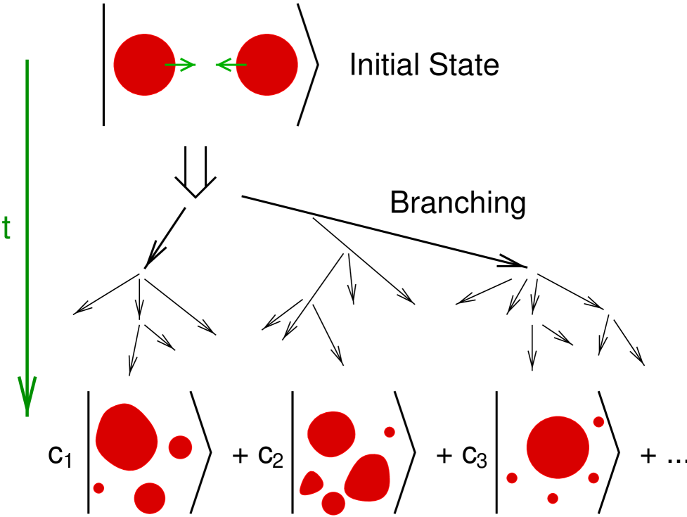
FIG. 1.: A schematic picture of the quantum branching processes for multichannel reactions.

As is well known, TDHF is not suitable for the reactions with many channels such as multifragmentation because it does not take account of the quantum branchings mentioned above. Although a single Slater determinant may be sufficient for the initial two nuclei and the fragments in each final channel, it is far from sufficient for the superposition of the final channel wave functions. In such cases, what one can expect by solving the deterministic time evolution is, at best, that one of the possible channels appears as the final state. In bad cases, however, the obtained final state looks like none of the final channels. The latter may be the case for the TDHF application to the multifragmentation of an expanding system because the mean field gets weaker and weaker as the system expands widely and therefore the diffusing single particle wave functions will never relocalize to form clusters. It is dangerous to apply the mean field concept to dilute system where the system may be branching into channels whose mean fields should be different from channel to channel. The VUU equation can be regarded as one of the extensions of TDHF, where the two-body collision effect is introduced as a term in the equation of the one-body phase space distribution. However, since this collision term is a deterministic term to take account of the averaged effect of the two-nucleon collisions, the quantum branching effect is not included in the VUU equation. The Boltzmann Langevin approach [7, 8], on the other hand, introduced the fluctuation as a random term associated with the two-nucleon collisions, and it may be applicable to the multichannel reactions such as multifragmentation. However, it is difficult to understand that the real origin of the cluster formation were the fluctuation due to the two-nucleon collisions, because the two-nucleon collisions are rare in the expanding nuclear matter, while the cluster formation should take place even in the ideal situation where the nuclear matter is uniformly expanding without initial fluctuation.

On the contrary to the mean field models mentioned above, the molecular dynamics models restrict the channel wave function to an (antisymmetrized) product of wave packets. The shape of the wave packets are usually kept fixed and the many body wave function is parametrized only by the centroids of the wave packets. The benefit of this restriction is that we can avoid encountering the situation where the single particle wave functions have been expanded and then the mean field concept does not work any longer. In other words, the channel wave function in the molecular dynamics models are restricted so that it cannot be a mixture of many channels which should be treated independently rather than as a whole in a single wave function. In the quantum molecular dynamics (QMD) [3, 4] and the antisymmetrized molecular dynamics (AMD) [5, 6], the centroid motion in each channel is determined by the equation of motion derived from the time-dependent variational principle. In addition to it, the effect of the two-body collisions is introduced as a stochastic branching process, which brings the system from a single initial state to many possible final channels randomly. Because of these reasons, QMD and AMD are suitable frameworks for the fragmentation phenomena.

Many people have ever tried to extend the molecular dynamics models by generalizing the wave packets [9, 10, 11, 6], usually by treating the width parameters of the wave packets as dynamical variables as well as the wave packet centroids. Although this extension can be an improvement for some phenomena [11], it is rather a change for the worse in the context of multifragmentation. Such extension draws the molecular dynamics models close to a mean field model which fails into the pathological situation where many independent channels are mixed in a single Slater determinant. In fact, Kiderlen et al. [9] and Chomaz et al. [10] reported that the diffused wave packets never shrink again to form clusters in a hot expanding nuclear system.

In Ref. [12], we took a different way to extend AMD by taking account of the precise one-body dynamics without losing the benefit of the molecular dynamics models that the channel wave function cannot fall into a mixture of many channels. It was achieved not by generalizing the channel wave function but by introducing the wave packet diffusion effect as a new quantum branching process. This extended AMD is called AMD-V, since the wave packet diffusion effect is calculated with the Vlasov equation [14]. When a expanding system is calculated by AMD-V, one can imagine that not only the centroids expand but also the successive quantum branchings take place due to the wave packet diffusion effect, and that the multifragment channels appear stochastically. In fact, we showed in Refs. [12, 13] that AMD-V works very well for the multifragmentation in ${}^{40}{\mathrm{Ca}}+{}^{40}{\mathrm{Ca}}$ reaction at 35 MeV/nucleon, though the expansion in this case is not spherical but mainly in the beam direction like the neck fragmentation. The wave packet diffusion process is also related to the nucleon emission rate and the energy carried out by emitted nucleons, which was essential for the correct prediction of the excitation energies of the produced fragments. No other microscopic models have ever reproduced these fragmentation data so nicely.

Ohnishi and Randrup take yet another approach to improve the molecular dynamics models [15]. Based on the idea that the essential part of the multifragmentation is governed by the statistical effect, they introduced a fluctuation-dissipation term to the equation of motion by hand so as to ensure the correct equilibrium property. Although the good statistics is the advantage of their model, there is no microscopic and dynamical background for the added fluctuation-dissipation term. We would like to emphasize here that their approach is not the unique way to get the quantum statistics in the molecular dynamics. Even though we start with the microscopic dynamical consideration, it is possible to get the quantum statistics as shown in Refs. [16, 17].

In spite of the fact that interesting high-quality multifragmentation data were published for heavy system such as ${}^{197}\!{\mathrm{Au}}+{}^{197}\!{\mathrm{Au}}$ collisions [18], no satisfactory explanation by microscopic dynamical models has been given. This difficulty is due to the essentially quantum mechanical feature of multifragmentation. Although AMD-V is one of few realistic models that have possibility to reproduce the data, it was impossible so far to apply AMD to heavy systems because of the reason of CPU time. The main purpose of this paper is, therefore, to give a framework of AMD-V whose numerical calculation is feasible even for ${}^{197}\!{\mathrm{Au}}+{}^{197}\!{\mathrm{Au}}$ collisions, by introducing an improvement and an approximation to the original AMD-V framework.

The necessary CPU time of the original AMD calculation is proportional to the forth power of the mass number of the system. This means that the required CPU time for ${}^{197}\!{\mathrm{Au}}+{}^{197}\!{\mathrm{Au}}$ reactions is about 600 times as much as for ${}^{40}{\mathrm{Ca}}+{}^{40}{\mathrm{Ca}}$ reactions. In order to overcome this problem, we introduce in this paper a new approximation for the AMD Hamiltonian which can be evaluated with the CPU time proportional to the third power of the mass number. This approximation is called the triple-loop approximation.

In the original AMD-V calculation of Ref. [12], the most time-consuming part was the procedure to ensure the energy conservation after the quantum branching process due to the wave packet diffusion effect. It was necessary to solve a kind of frictional cooling equation at least for several time steps to search the energy conserving point. This procedure becomes unnecessary and the framework becomes more transparent in this paper when the wave packet diffusion effect is reformulated as a random term in a Langevin-type equation of motion, the formal structure of which is similar to the equation by Ohnishi and Randrup [15].

This paper is organized as follows. In Sec. II, the framework of the improved AMD-V is given. Especially the wave packet diffusion process is formulated as a random term in the equation of motion. In Sec. III, the triple-loop approximation for the AMD Hamiltonian is formulated and some tests for this approximation are given. A demonstrative calculation for ${}^{197}\!{\mathrm{Au}}+{}^{197}\!{\mathrm{Au}}$ collisions at 150 MeV/nucleon is given in Sec. IV in order to show that the AMD-V calculation for heavy system is really possible and it is likely to reproduce the multifragmentation data. Section V is devoted for the summary.

II Framework of AMD with Quantum Branching Processes

In constructing a time-dependent quantum model for medium energy heavy ion collisions, one should keep in mind the fact that the initial state branches into a huge number of reaction channels in the intermediate states and the final state. It is too difficult to follow the time evolution of the total many-body wave function in which the many-body correlations are not negligible. Therefore, we treat separately the branching into channels and the time evolution within each channel. Approximations such as the mean field theory may be valid within each channel, while the interference among the branched channels may be unimportant. The independence of the time evolution of each channel should be respected.

A Channel wave function and equation of motion

We describe each channel wave function by an AMD wave function which is a single Slater determinant of Gaussian wave packets [5],

$$\Phi(Z)=\det\Bigl{[}\exp\Bigl{\{}-\nu\Bigl{(}{\mathbf{r}}_{j}-\frac{{\mathbf{Z}}_{i}}{\sqrt{\nu}}\Bigr{)}^{2}+\frac{1}{2}{\mathbf{Z}}_{i}^{2}\Bigr{\}}\chi_{\alpha_{i}}(j)\Bigr{]},$$ (1)

where the complex variables $Z\equiv\{{\mathbf{Z}}_{i};\ i=1,\ldots,A\}=\{Z_{i\sigma};\ i=1,\ldots,A,\ \sigma=x,y,z\}$ represent the centroids of the wave packets. We take the width parameter $\nu=0.16$ $\mathrm{fm}^{-2}$ and the spin isospin states $\chi_{\alpha_{i}}=p\uparrow$, $p\downarrow$, $n\uparrow$, or $n\downarrow$.

The AMD wave function (1) seems to be very simple, but it is sufficient for the description of the ground states of nuclei. For example, the binding energies obtained by the frictional cooling method [19] coincide with the experimental data within the precision of 1 MeV/nucleon even though the common values of $\nu$ and $T_{0}$ (mentioned later) are used for all nuclei [20]. Therefore the initial state of the reaction and the individual channel wave functions in the intermediate and final states are well described by the AMD wave functions.

The time evolution of the wave packet centroids $Z$ within the same channel is determined by the time dependent variational principle,

$$\delta\int dt\,{\langle\Phi(Z)|(i\hbar{d\over dt}-H)|\Phi(Z)\rangle\over\langle\Phi(Z)|\Phi(Z)\rangle}=0,$$ (2)

from which one can derive the equation of motion for $Z$,

$$i\hbar\sum_{j\tau}C_{i\sigma,j\tau}{dZ_{j\tau}\over dt}={\partial{\mathcal{H}}\over\partial Z_{i\sigma}^{*}}.$$ (3)

$C_{i\sigma,j\tau}$ with $\sigma,\tau=x,y,z$ is a hermitian matrix defined by

$$C_{i\sigma,j\tau}=\frac{\partial^{2}}{\partial Z_{i\sigma}^{*}\partial Z_{j\tau}}\log\langle\Phi(Z)|\Phi(Z)\rangle,$$ (4)

and $\cal H$ is the expectation value of the Hamiltonian after the subtraction of the spurious kinetic energy of the zero-point oscillation of the center-of-masses of fragments [5],

$${\cal H}(Z)=\frac{\langle\Phi(Z)|H|\Phi(Z)\rangle}{\langle\Phi(Z)|\Phi(Z)\rangle}-\frac{3\hbar^{2}\nu}{2M}A+T_{0}(A-N_{\mathrm{F}}(Z)).$$ (5)

The quantum Hamiltonian

$$H=\sum_{i=1}^{A}\frac{{\mathbf{p}}_{i}^{2}}{2M}+\sum_{i<j}v_{ij}$$ (6)

includes an effective two-body interaction such as the Gogny force [21] which can be density dependent, since the model wave function is limited to a single Slater determinant. The spurious kinetic energies of the zero-point oscillation of the center-of-mass of the isolated fragments and nucleons have been subtracted in Eq. (5) by introducing a continuous number of fragments $N_{\mathrm{F}}(Z)$ [5]. Without this subtraction, the Q-values for nucleon emissions and fragmentations would not be reproduced. The parameter $T_{0}$ is $3\hbar^{2}\nu/2M$ in principle but treated as a free parameter for the adjustment of the binding energies. Once the zero-point kinetic energies have been subtracted, the center-of-mass wave function of an isolated fragment (or nucleon) should be regarded as a plane wave. This method, however, only takes account of the expectation value of the kinetic energy and ignores its quantum fluctuation. This point will be reconsidered in the next subsection.

For the later formulation, it is convenient to introduce the Poisson bracket $\{{\mathcal{F}},{\mathcal{G}}\}$ and the inner product of the canonical gradients $({\mathcal{F}},{\mathcal{G}})$,

$$\{{\mathcal{F}},{\mathcal{G}}\} = \frac{1}{i\hbar}\sum_{i\sigma,j\tau}\frac{\partial{\mathcal{F}}}{\partial Z_{i\sigma}}C^{-1}_{i\sigma,j\tau}\frac{\partial{\mathcal{G}}}{\partial Z_{j\tau}^{*}}$$ (8)

$$-\frac{1}{i\hbar}\sum_{i\sigma,j\tau}\frac{\partial{\mathcal{G}}}{\partial Z_{i\sigma}}C^{-1}_{i\sigma,j\tau}\frac{\partial{\mathcal{F}}}{\partial Z_{j\tau}^{*}},$$

$$({\mathcal{F}},{\mathcal{G}}) = \frac{1}{\hbar}\sum_{i\sigma,j\tau}\frac{\partial{\mathcal{F}}}{\partial Z_{i\sigma}}C^{-1}_{i\sigma,j\tau}\frac{\partial{\mathcal{G}}}{\partial Z_{j\tau}^{*}}$$ (10)

$$+\frac{1}{\hbar}\sum_{i\sigma,j\tau}\frac{\partial{\mathcal{G}}}{\partial Z_{i\sigma}}C^{-1}_{i\sigma,j\tau}\frac{\partial{\mathcal{F}}}{\partial Z_{j\tau}^{*}}.$$

Then the equation of motion (3) can be rewritten as

$$\dot{Z}=\{Z,{\mathcal{H}}\}.$$ (11)

On the other hand, the frictional cooling equation can be written as

$$\dot{Z}=\lambda\{Z,{\mathcal{H}}\}+\mu(Z,{\mathcal{H}}),$$ (12)

for which one can show that the energy expectation value decreases as time

$$\dot{\mathcal{H}}=\mu({\mathcal{H}},{\mathcal{H}})\leq 0$$ (13)

for arbitrary $\lambda$ and $\mu(<0)$.

The one-body Wigner function for the AMD wave function (1) is given by

$$f({\mathbf{r}},{\mathbf{p}}) = 8\sum_{ik}e^{-2({\mathbf{u}}^{*}-{\mathbf{Z}}_{i}^{*})\cdot({\mathbf{u}}-{\mathbf{Z}}_{k})}B_{ik}B^{-1}_{ki},$$ (14)

$${\mathbf{u}} = \sqrt{\nu}\,{\mathbf{r}}+\frac{i}{2\hbar\sqrt{\nu}}{\mathbf{p}},$$ (15)

where

$$B_{ik}=e^{{\mathbf{Z}}_{i}^{*}\cdot{\mathbf{Z}}_{k}}\delta_{\alpha_{i}\alpha_{k}}$$ (16)

is the overlap matrix of the non-orthogonal single particle wave packets in Eq. (1). In what follows, it is sometimes convenient to introduce a QMD-like approximation,

$$f({\mathbf{r}},{\mathbf{p}})\approx 8\sum_{i}e^{-2|{\mathbf{u}}-{\mathbf{W}}_{i}|^{2}},$$ (17)

by using the physical coordinate $W=\{{\mathbf{W}}_{i}\}$ [5] defined by

$${\mathbf{W}}_{i}=\sum_{j=1}^{A}\Bigl{(}\sqrt{Q}\Bigr{)}_{ij}{\mathbf{Z}}_{j},\quad Q_{ij}=B_{ij}B^{-1}_{ji}.$$ (18)

The coordinates $W$ can be regarded as physical ones because quantities such as the orbital angular momentum and the number of the harmonic-oscillator quanta are written in the usual way by using $W$. Furthermore the coordinates $W$ are canonical coordinates when the antisymmetrization among more than two packets is negligible. The physical coordinates are very useful in various places of the formulation of AMD-V, while the QMD-like approximation of Eq. (17) is too poor to be useful in the evaluation of the Hamiltonian as will be seen in Sec. III.

B Wave packet diffusion process

The wave packet shape is not allowed to change in AMD. Therefore the dynamics of the single particle wave functions is not so precisely described as in TDHF. However, we should not extend AMD to TDHF because TDHF has the pathological problem of the spurious coupling of channels. In Ref. [12], instead of extending the channel wave functions, we introduced the precise single particle dynamics into AMD as a new stochastic branching process. In this subsection, this process is reformulated as a random term of a Langevin-type equation of motion which is more suitable for numerical calculations.

1 Fluctuation due to the wave packet diffusion

Each nucleon $k$ in an AMD wave function $\Phi(Z(t))$ of one of the branches at the time $t$ is represented approximately by a Gaussian wave packet in phase space

$$f_{k}(x,t)=8\,\exp\Bigl{[}-2\sum_{a=1}^{6}(x_{a}-X_{ka}(t))^{2}\Bigr{]},$$ (19)

where we have introduced the 6-dimensional phase space coordinate

$$\{x_{a};\ a=1,\ldots,6\}=\{\sqrt{\nu}\,{\mathbf{r}},{\mathbf{p}}/2\hbar\sqrt{\nu}\}.$$ (20)

The centroid $\{X_{ka};\ a=1,\ldots,6\}$ stands for the physical coordinate ${\mathbf{W}}_{k}$. In the usual AMD, the time evolution of $X_{ka}$ is derived from the equation of motion while the shape of the wave packet is fixed.

However, more reliable time evolution of the one-body distribution function is given by the TDHF equation or the Vlasov equation [14],

$${\partial f_{k}\over\partial t}+{\partial h\over\partial{\mathbf{p}}}\cdot{\partial f_{k}\over\partial{\mathbf{r}}}-{\partial h\over\partial{\mathbf{r}}}\cdot{\partial f_{k}\over\partial{\mathbf{p}}}=0.$$ (21)

Writing the expectation value of the Hamiltonian as ${\mathcal{H}}[f]$ for a Slater determinant represented by $f({\mathbf{r}},{\mathbf{p}})$, one can obtain the single-particle Hamiltonian $h$ by

$$h({\mathbf{r}},{\mathbf{p}},t)=\frac{\delta{\mathcal{H}}[f]}{\delta f({\mathbf{r}},{\mathbf{p}})}\bigg{|}_{f=f({\mathbf{r}},{\mathbf{p}},t)},$$ (22)

for the AMD wave function $\Phi(Z(t))$ whose Wigner function is given by Eq. (14). The time derivative of the width and shape of the wave packet

$$\dot{\sigma}^{2}_{kab}(t)\equiv\frac{d}{dt}\int\Bigl{(}x_{a}-X_{ka}(t)\Bigr{)}\Bigl{(}x_{b}-X_{kb}(t)\Bigr{)}f_{k}(x,t)d^{6}x$$ (23)

can be evaluated based on the Vlasov equation (21) by using the test particle method or by the direct analytical calculation.

It will be useful to note that the wave packet diffusion $\dot{\sigma}^{2}_{kab}$ is mainly determined by the curvature of the mean field in $h({\mathbf{r}},{\mathbf{p}})$ in the region around the wave packet $k$. When the potential is quadratic with the curvature $\frac{1}{2}m\omega^{2}=2\hbar^{2}\nu^{2}/m$, the wave packet diffusion effect is exactly zero, which is approximately satisfied for the packets inside the nucleus. On the other hand, for the packets near the surface of the nucleus, the potential curvature is negative and then the wave packet diffusion effect becomes essential.

Instead of changing the shape of the wave packet $f_{k}$, we now give fluctuation $\delta X_{ka}(t)$ to the centroid $X_{ka}(t)$ in order to introduce the wave packet diffusion effect $\dot{\sigma}^{2}_{k}$. If we assume the white noise for the fluctuation, it should satisfy

$$\overline{\delta X_{ka}(t)} = 0,$$ (24)

$$\overline{\delta X_{ka}(t)\delta X_{kb}(t^{\prime})} = [\dot{\sigma}^{2}_{k}]_{ab}(t)\delta(t-t^{\prime}).$$ (25)

The negative eigenvalues of $\dot{\sigma}^{2}_{k}$ have been replaced by zero because the shrinking of the wave packet cannot be treated unless we respect the interference among channels.

Although the higher moments of the fluctuation can also be calculated with the Vlasov equation, we expect that their effect is not important. In our early work [12], we took the distribution function for the fluctuation $\xi_{a}\equiv\delta X_{ka}$,

$$P(\xi) = (1-c)\delta(\xi)+c\frac{\sqrt{\det\alpha}}{(\pi/2)^{3}}\exp\Bigl{(}-2\sum_{ab}\xi_{a}\alpha_{ab}\xi_{b}\Bigr{)},$$ (27)

$$\alpha_{ab}\equiv\frac{\mathop{\mathrm{tr}}[\dot{\sigma}^{2}_{k}]}{3}[\dot{\sigma}^{2}_{k}]^{-1}_{ab},$$

where $c$ is chosen to give the correct variance of the fluctuation [Eq. (25)]. Since $\alpha$ is of the order of 1, a big branching takes place with small probability, while no branching takes place in most cases. However, we here take the Gaussian distribution

$$P(\xi) = \frac{\sqrt{\det\alpha^{\prime}}}{(\pi/2)^{3}}\exp\Bigl{(}-2\sum_{ab}\xi_{a}\alpha^{\prime}_{ab}\xi_{b}\Bigr{)},$$ (29)

$$\alpha^{\prime}_{ab}\equiv c^{\prime}[\dot{\sigma}^{2}_{k}]^{-1}_{ab},$$

where $c^{\prime}$ is determined by Eq. (25), because this is more convenient for the numerical calculation. In this case, a small fluctuation is given to each centroid at every time step.

It should be noted that the fluctuation $\delta X_{ka}(t)$ is spurious for an isolated wave packet $k$ because there is no other packets that can absorb the recoil from the fluctuation. Furthermore the mean field theory [Eq. (21)] is not necessarily valid for light nuclei with $A\lesssim 10$. We should avoid the situation where the unreliable fluctuation for the packets inside a light fragment has a drastic effect on the dynamics such as spuriously breaking the fragment. Therefore, by checking the packets in the neighborhood of the packet $k$, we put $\delta X_{ka}(t)=0$ when

$$\sum_{i}\theta\Bigl{(}1.75-|\mathop{\mathrm{Re}}({\mathbf{Z}}_{i}-{\mathbf{Z}}_{k})|\Bigr{)}\leq 10$$ (31)

and

$$\biggl{|}\sum_{i}\theta\Bigl{(}1.75-|\mathop{\mathrm{Re}}({\mathbf{Z}}_{i}-{\mathbf{Z}}_{k})|\Bigr{)}\mathop{\mathrm{Re}}({\mathbf{Z}}_{i}-{\mathbf{Z}}_{k})\biggr{|}\leq 5.$$ (32)

Although this prescription may make the cooling of light fragments too slow, it is not a problem practically because the decay of these fragments can be calculated later by a statistical decay code.

For numerical convenience, we now introduce a small delay time $\tau$ of the response to the fluctuation $\delta X_{ka}$. The delayed fluctuation $\Xi_{ka}$ is obtained by the equation

$$\frac{d}{dt}\Xi_{ka}(t)=\frac{1}{\tau}\delta X_{ka}(t)-\frac{1}{\tau}\Xi_{ka}(t),$$ (33)

whose solution is

$$\Xi_{ka}(t)=\frac{1}{\tau}\int_{0}^{t}\delta X_{ka}(t^{\prime})e^{-(t-t^{\prime})/\tau}dt^{\prime},$$ (34)

by assuming $\Xi_{ka}(0)=0$ for the initial state. Instead of the original fluctuation $\delta X_{ka}(t)$, this delayed fluctuation $\Xi_{ka}(t)$ is to be added to the centroid $X_{ka}(t)$. In numerical calculations we take $\tau=5$ fm/$c$, which should be smaller than the important time scales of the reaction. Since the fluctuation is smoothened by the averaging over the time $\tau$, it can be treated easily numerically.

Some readers may be interested in the difference between the fluctuation introduced by Ohnishi and Randrup [15] and that of our present work. In our model, the fluctuations of different packets (labeled by $k$) are independent while the correlations of the phase space components (labeled by $a$ and $b$) of each packet is properly incorporated by Eq. (25). This is a natural consequence of the fact that our fluctuation is introduced based on the mean field model. On the contrary, Ohnishi and Randrup simply ignores the importance of the phase space correlations, while they introduce the correlations among different packets without any microscopic or dynamical justification.

2 Equation of motion and conserved quantities

The above determined fluctuation $\Xi_{ka}(t)$ or its complex vector representation $\mathchoice{{\hbox{\boldmath$\displaystyle\Xi$}}}{{\hbox{\boldmath$\textstyle\Xi$}}}{{\hbox{\boldmath$\scriptstyle\Xi$}}}{{\hbox{\boldmath$\scriptscriptstyle\Xi$}}}_{k}(t)$ is the fluctuation to the physical coordinate ${\mathbf{W}}_{k}$. In order to put it in the equation of motion, it is now necessary to convert it to the fluctuation to the original AMD coordinates $Z$. For this purpose let us introduce a time-dependent one-body hermitian operator $\hat{o}_{k}(t)$ that generates the fluctuation $\mathchoice{{\hbox{\boldmath$\displaystyle\Xi$}}}{{\hbox{\boldmath$\textstyle\Xi$}}}{{\hbox{\boldmath$\scriptstyle\Xi$}}}{{\hbox{\boldmath$\scriptscriptstyle\Xi$}}}_{k}(t)$. The form of $\hat{o}_{k}(t)$ is taken as

$$\hat{o}_{k}(t)=i\sum_{j=1}^{A}\Bigl{\{} ({\mathbf{y}}_{kj}(t)\cdot\hat{{\mathbf{a}}}^{\dagger})|{\mathbf{W}}_{j}(t)\rangle\langle{\mathbf{W}}_{j}(t)|$$ (36)

$$-|{\mathbf{W}}_{j}(t)\rangle\langle{\mathbf{W}}_{j}(t)|({\mathbf{y}}_{kj}^{*}(t)\cdot\hat{{\mathbf{a}}})\Bigr{\}},$$

where the stochastic complex parameters $\{{\mathbf{y}}_{kj}(t);\ j=1,\ldots,A\}$ are to be determined below, and

$$\hat{\mathbf{a}} = \sqrt{\nu}\,\hat{\mathbf{r}}+\frac{i}{2\hbar\sqrt{\nu}}\hat{\mathbf{p}},$$ (37)

$$\langle{\mathbf{r}}|{\mathbf{W}}\rangle \propto \exp\Bigl{\{}-\nu\Bigl{(}{\mathbf{r}}-\frac{\mathbf{W}}{\sqrt{\nu}}\Bigr{)}^{2}\Bigr{\}}.$$ (38)

In QMD-like approximation by the use of the physical coordinates, the expectation value of this one-body operator is calculated as

$${\mathcal{O}}^{\prime}_{k}(W,t)=\sum_{i=1}^{A}\langle{\mathbf{W}}_{i}|\hat{o}_{k}|{\mathbf{W}}_{i}\rangle$$ (39)

$$\quad=i\sum_{ij}({\mathbf{y}}_{kj}(t)\cdot{\mathbf{W}}_{i}^{*}-{\mathbf{y}}_{kj}^{*}(t)\cdot{\mathbf{W}}_{i})e^{-|{\mathbf{W}}_{j}(t)-{\mathbf{W}}_{i}|^{2}}$$ (40)

By identifying the physical coordinates $W$ with the canonical coordinates, the stochastic parameters $\{{\mathbf{y}}_{kj}(t)\}$ are determined by the requirement that the one-body operator generates the fluctuation $\mathchoice{{\hbox{\boldmath$\displaystyle\Xi$}}}{{\hbox{\boldmath$\textstyle\Xi$}}}{{\hbox{\boldmath$\scriptstyle\Xi$}}}{{\hbox{\boldmath$\scriptscriptstyle\Xi$}}}_{k}(t)$ at the moment $t$,

$$i\hbar\delta_{ik}\mathchoice{{\hbox{\boldmath$\displaystyle\Xi$}}}{{\hbox{\boldmath$\textstyle\Xi$}}}{{\hbox{\boldmath$\scriptstyle\Xi$}}}{{\hbox{\boldmath$\scriptscriptstyle\Xi$}}}_{k}(t)=\frac{\partial{\mathcal{O}}^{\prime}_{k}(t)}{\partial{\mathbf{W}}_{i}^{*}}\biggl{|}_{W=W(t)}.$$ (41)

Then the fluctuation for $Z$ should be generated as $\{Z,{\mathcal{O}}_{k}(t)\}$ by the exact expectation value of the same one-body operator,

$${\mathcal{O}}_{k}(Z,t) = \frac{\langle\Phi(Z)|\hat{O}_{k}(t)|\Phi(Z)\rangle}{\langle\Phi(Z)|\Phi(Z)\rangle},$$ (42)

$$\hat{O}_{k}(t) = \sum_{i=1}^{A}\hat{o}_{ki}(t).$$ (43)

Before putting the fluctuation $\{Z,{\mathcal{O}}_{k}(t)\}$ in the equation of motion, we should note the fact that the fluctuation violates the conservation lows for the total momentum and the total energy. Such conservation lows should be achieved through many-body correlations in reality. Since this kind of many-body correlations are beyond the scope of the one-body dynamics of the Vlasov equation, it is inevitable to introduce the conservation lows by hand. By correcting the fluctuation for the conservation lows, the equation of motion of AMD-V is now written as

$$\dot{Z}=\{Z,{\mathcal{H}}\}+\sum_{k=1}^{A}\gamma_{k}\biggl{[}\Bigl{\{}Z,\;{\mathcal{O}}_{k}+\sum_{m}\alpha_{km}{\mathcal{P}}_{m}\Bigr{\}}_{{\mathrm{C}}_{k}}$$ (44)

$$+\mu_{k}\Bigl{(}Z,\;{\mathcal{H}}+\sum_{m}\beta_{km}{\mathcal{Q}}_{m}\Bigr{)}_{{\mathrm{N}}_{k}} \biggr{]}.$$ (45)

The first term in the square bracket is the fluctuation due to $\mathchoice{{\hbox{\boldmath$\displaystyle\Xi$}}}{{\hbox{\boldmath$\textstyle\Xi$}}}{{\hbox{\boldmath$\scriptstyle\Xi$}}}{{\hbox{\boldmath$\scriptscriptstyle\Xi$}}}_{k}$ corrected for the center-of-mass coordinate and momentum conservation, and the second term is the cooling (or heating) term to ensure the energy conservation. The parameter $\gamma_{k}$ can be regarded as 1 until its meaning is explained later.

When the system has been decomposed into several clusters, the fluctuation $\mathchoice{{\hbox{\boldmath$\displaystyle\Xi$}}}{{\hbox{\boldmath$\textstyle\Xi$}}}{{\hbox{\boldmath$\scriptstyle\Xi$}}}{{\hbox{\boldmath$\scriptscriptstyle\Xi$}}}_{k}$ to a packet $k$ in one of the clusters should not affect the packets in the other clusters through the conservation lows. In order to ensure this point, we define the cluster ${\mathrm{C}}_{k}$ which includes the packet $k$, where the clusters are identified by the condition that two packets $i$ and $j$ belong to the same cluster if $|{\mathbf{Z}}_{i}-{\mathbf{Z}}_{j}|<1.75$. The subscript ${\mathrm{C}}_{k}$ of the Poisson bracket in Eq. (45) indicates that the centroids of the packets in the other clusters are treated as static parameters. Namely, the packets in the other clusters are omitted in the summation in Eq. (8), and $C^{-1}$ is replaced by the inverse matrix of the submatrix of $C$. In Eq. (45), by using the Lagrange multipliers $\alpha_{m}$, the constraints are introduced for the conserved quantities $\{{\mathcal{P}}_{m}\}$, which are the three components of the center-of-mass coordinate and the three components of the total momentum

$$\bigl{<}\frac{1}{A}\sum_{i}{\mathbf{r}}_{i}\bigr{>} = \frac{1}{A}\sum_{i}\mathop{\mathrm{Re}}{\mathbf{Z}}_{i}/\sqrt{\nu},$$ (46)

$$\bigl{<}\sum_{i}{\mathbf{p}}_{i}\bigr{>} = \sum_{i}2\hbar\sqrt{\nu}\mathop{\mathrm{Im}}{\mathbf{Z}}_{i}.$$ (47)

Then the Lagrange multipliers should be determined by

$$\{{\mathcal{P}}_{l},{\mathcal{O}}_{k}\}_{{\mathrm{C}}_{k}}+\sum_{m}\{{\mathcal{P}}_{l},{\mathcal{P}}_{m}\}_{{\mathrm{C}}_{k}}\alpha_{km}=0.$$ (48)

The method to ensure the energy conservation should be considered carefully, because it has more drastic effects than the center-of-mass conservation. The set of the packets ${\mathrm{N}}_{k}$ which can be adjusted in order to cancel the energy violation by $\mathchoice{{\hbox{\boldmath$\displaystyle\Xi$}}}{{\hbox{\boldmath$\textstyle\Xi$}}}{{\hbox{\boldmath$\scriptstyle\Xi$}}}{{\hbox{\boldmath$\scriptscriptstyle\Xi$}}}_{k}$ is restricted to the neighborhood of the packet $k$ defined by

$${\mathrm{N}}_{k}=\{i;\ |{\mathbf{Z}}_{i}-{\mathbf{Z}}_{k}|<2.5\ \mbox{and}\ i\in{\mathrm{C}}_{k}\ \mbox{and}\ i\neq k\}.$$ (49)

The total energy is restored by the frictional cooling term in Eq. (45) with $\mu_{k}$ adjusted for the conservation. Since this cooling term should not violate the other conservation lows, the quantities

$$\{{\mathcal{Q}}_{m}\}=\Bigl{\{}\bigl{<}\sum_{i}{\mathbf{r}}_{i}\bigr{>},\ \bigl{<}\sum_{i}{\mathbf{p}}_{i}\bigr{>},\ \bigl{<}\sum_{i}{\mathbf{r}}_{i}\times{\mathbf{p}}_{i}\bigr{>}\Bigr{\}}$$ (50)

are kept constant by determining the Lagrange multipliers $\beta_{km}$ by

$$({\mathcal{Q}}_{l},{\mathcal{H}})_{{\mathrm{N}}_{k}}+\sum_{m}({\mathcal{Q}}_{l},{\mathcal{Q}}_{m})_{{\mathrm{N}}_{k}}\beta_{km}=0.$$ (51)

The parameter $\mu_{k}$ is then determined by

$$\mu_{k}=-\frac{\{{\mathcal{H}},\;{\mathcal{O}}_{k}+\sum_{m}\alpha_{km}{\mathcal{P}}_{m}\}_{{\mathrm{C}}_{k}}}{({\mathcal{H}},\;{\mathcal{H}}+\sum_{m}\beta_{km}{\mathcal{Q}}_{m})_{{\mathrm{N}}_{k}}}$$ (52)

in order to conserve the total energy.

It should be noted that $\mu_{k}$ appear in Eq. (45) only through their summation $\mu\equiv\sum_{k}\mu_{k}$ if the constrains are ignored for simplicity. Since $\mu$ is an intensive quantity (which is independent of the size of the system) and it is averaged over many independent fluctuations ${\mathcal{O}}_{k}$, one can replace $\mu$ with its averaged value $\bar{\mu}$ which is a function of the current state $Z$. Then the cooling term of Eq. (45) is formally similar to the dissipation term of the Langevin equation that Ohnishi and Randrup proposed to introduce together with the fluctuation term [15]. However, we use Eq. (52) directly without replacing $\mu_{k}$ with their averaged values, so that the total energy is exactly conserved. Furthermore, in our method, we do not need to evaluate the second derivatives of the Hamiltonian ${\mathcal{H}}$ which would be necessary in order to directly evaluate the averaged value $\bar{\mu}$.

The method of the energy conservation is the most difficult ambiguity of this model because it is an effect beyond the mean field theories. The above prescription, therefore, intend to achieve the energy conservation with the least modification of the other degrees of freedom by moving them in the direction of the canonical gradient of the Hamiltonian. However, as discussed in Ref. [12], it seems that the adjusted degrees of freedom should be restricted to the thermal or single-particle ones in order to avoid the unphysical direct energy conversion from the collective energy (such as the incident energy of the heavy ion collision) to the single-particle energy of the fluctuation. For this purpose, the monopole and the quadrupole moments in the coordinate and momentum spaces

$$\bigl{<}\sum_{i}{\mathbf{r}}_{i}{\mathbf{r}}_{i}\bigr{>},\ \bigl{<}\sum_{i}{\mathbf{p}}_{i}{\mathbf{p}}_{i}\bigr{>}$$ (53)

are also included in $\{{\mathcal{Q}}_{m}\}$ when ${\mathrm{N}}_{k}$ is composed of more than 15 packets.

For an isolated packet $k$, we have put $\delta X_{ka}=0$. However, due to the delay time $\tau$, the delayed fluctuation $\mathchoice{{\hbox{\boldmath$\displaystyle\Xi$}}}{{\hbox{\boldmath$\textstyle\Xi$}}}{{\hbox{\boldmath$\scriptstyle\Xi$}}}{{\hbox{\boldmath$\scriptscriptstyle\Xi$}}}_{k}$ may not be zero and should be respected even for an isolated packet. Therefore, when $N_{k}\leq 4$ with $N_{k}$ being the number of the element of ${\mathrm{N}}_{k}$, we search the non-isolated wave packet $i$ ($N_{i}>4$) that is the closest to the packet $k$, and then ${\mathrm{N}}_{i}\cup{\mathrm{N}}_{k}\cup\{i\}$ and ${\mathrm{C}}_{i}\cup\{k\}$ are used instead of ${\mathrm{N}}_{k}$ and ${\mathrm{C}}_{k}$, respectively, in the above formalism.

Finally we comment on the necessary correction when the system is near the ground state. As already discussed in Ref. [12], the fluctuation is small but not exactly zero even for the ground state because of the semiclassical nature of the Vlasov equation and the restricted Slater determinant in AMD. Since the fluctuation should be zero in the ground state, a reduction factor $\gamma_{k}$ is introduced in Eq. (45) in order to cancel the fluctuation only near the ground state. By noting that the cooling term becomes zero for the ground state, a measure of the difference from the ground state is introduced by

$$D_{k}\equiv\frac{6}{6N_{k}-N_{\mathrm{cons}}}\Bigl{(}{\mathcal{H}},\;{\mathcal{H}}+\sum_{m}\beta_{km}{\mathcal{Q}}_{m}\Bigr{)}_{{\mathrm{N}}_{k}},$$ (54)

where $N_{\mathrm{cons}}$ denotes the number of the constrained quantities $\{{\mathcal{Q}}_{m}\}$, and therefore $6N_{k}-N_{\mathrm{cons}}$ is the number of the free degrees of freedom for the energy adjustment. The reduction factor $\gamma_{k}$ is then taken as

$$\gamma_{k} = \frac{1}{\sqrt{1+(\mu_{k}/\mu_{0k})^{2}}},$$ (55)

$$\mu_{0k} = \frac{1200}{6N_{k}-N_{\mathrm{cons}}}\sqrt{\frac{5\ \mathrm{fm}/c}{\tau}}\biggl{(}\frac{D_{k}}{0.1\ \mathrm{MeV}/(\mathrm{fm}/c)}\biggr{)}^{3},$$ (56)

so that the coefficient for the cooling term $\gamma_{k}|\mu_{k}|$ does not exceed the upper limit $\mu_{0k}$. The purpose of the dependence of $\mu_{0k}$ on $(6N_{k}-N_{\mathrm{cons}})$ and $\tau$ is to make this reduction effect independent of the choice of the neighborhood ${\mathrm{N}}_{k}$ [Eq. (49)] and the delay time $\tau$. With this parameterization, the fluctuation is reduced to zero in the ground state, while there is almost no reduction soon after hard two-nucleon collisions in the example of ${}^{197}\!{\mathrm{Au}}+{}^{197}\!{\mathrm{Au}}$ collisions shown in Sec. IV.

3 Energy fluctuation of emitted packets

As already discussed, we have subtracted the zero-point kinetic energies of isolated packets in Eq. (5). Therefore the emitted packet $k$ should be regarded as a plane wave of the momentum ${\mathbf{P}}_{k}=2\hbar\sqrt{\nu}\mathop{\mathrm{Im}}{\mathbf{Z}}_{k}$. This is convenient than treating it as a Gaussian packet with a momentum spread because the nucleons in the final channels are usually observed experimentally as momentum and energy eigen states and we should ensure the momentum and the energy conservations in each cannel.

Let us consider the case where a wave packet $k$ would be emitted as a whole with the momentum centroid value ${\mathbf{P}}_{0k}$ when the zero-point kinetic energy were not subtracted from the Hamiltonian. The momentum of this nucleon is

$${\mathbf{p}}_{k}={\mathbf{P}}_{0k}+{\mathbf{q}},$$ (57)

where ${\mathbf{q}}$ is a random number of the Gaussian distribution with $\langle{\mathbf{q}}\rangle=0$ and $\langle q_{\sigma}q_{\tau}\rangle=\hbar^{2}\nu\delta_{\sigma\tau}$ for $\sigma,\tau=x,y,z$. The kinetic energy of this wave packet is then

$$E_{k}=\frac{{\mathbf{P}}_{0k}^{2}}{2M}+\frac{{\mathbf{P}}_{0k}\cdot{\mathbf{q}}}{M}+\frac{{\mathbf{q}}^{2}}{2M}.$$ (58)

When the expectation value of the third term $\langle{\mathbf{q}}^{2}\rangle/2M=3\hbar^{2}\nu/2M$ is subtracted from the Hamiltonian, the added term in Eq. (5) acts as a repulsive force to this packet. Then it will be emitted with the momentum ${\mathbf{P}}_{k}$ that satisfies

$$\langle E_{k}\rangle=\frac{{\mathbf{P}}_{k}^{2}}{2M}=\frac{{\mathbf{P}}_{0k}^{2}}{2M}+\frac{3\hbar^{2}\nu}{2M}.$$ (59)

Namely the momentum ${\mathbf{P}}_{k}$ is larger than the true centroid ${\mathbf{P}}_{0k}$ while the energy expectation value does not change because of the absence of the momentum spread when the zero-point energy is subtracted.

This prescription, however, has a shortcoming that it takes account of only the expectation value of the kinetic energy and ignores its fluctuation. For a preequilibrium nucleon in high energy collisions, ${\mathbf{P}}_{0k}$ may be so large that the fluctuation of the second term of Eq. (58) may play some role though its expectation value is zero. In order to take account of this kind of energy fluctuation, we now introduce a random process when each packet is emitted. By neglecting the difference of the direction of ${\mathbf{P}}_{0k}$ and ${\mathbf{P}}_{k}$, the right amount of the energy fluctuation can be produced by changing the momentum as

$${\mathbf{P}}_{k}\rightarrow(P_{k}-\delta p_{k}+x\Delta p_{k}){\mathbf{P}}_{k}/P_{k},$$ (60)

where $x$ is a random number taken from the normal distribution with $\langle x\rangle=0$ and $\langle x^{2}\rangle=1$, and

$$\delta p_{k} = P_{k}-\sqrt{P_{k}^{2}-\hbar^{2}\nu},$$ (61)

$$\Delta p_{k} = \hbar\sqrt{\nu}$$ (62)

Not only the fluctuation ($\Delta p_{k}$) is given but also the average value of $P_{k}$ is decreased by $\delta p_{k}$ so that the energy expectation value does not change by this random process. It can be introduced as a new term in the equation for ${\mathbf{\Xi}}_{k}$ (33) which is put at the moment when the packet $k$ is isolated ($N_{k}=0$) for the first time. The momentum in the above discussion should be understood as the relative momentum between the emitted nucleon and the parent nucleus. The total energy conservation is achieved by adjusting other degrees of freedom of the parent nucleus just in the same way for the fluctuation due to the wave packet diffusion effect.

It should be emphasized here that the above prescription is taken when the wave packet is emitted as a whole with the considerably high momentum $P_{k}$, such as in the early stage of high energy collisions. On the other hand, when a low energy nucleon evaporates from a nucleus, what comes out of the nucleus is only a high momentum component of the packet as we discussed in Refs. [16, 17, 12]. Therefore, the true momentum spread around ${\mathbf{P}}_{k}$ should be small and the above prescription should not be taken in this case. In order to continuously connect these two extremes of high and low energies, Eqs. (61) and (62) are replaced by

$$\delta p_{k} = P_{k}-\sqrt{\max(P_{k}^{2}-\hbar^{2}\nu,\ P_{k}^{2}/4)},$$ (63)

$$\Delta p_{k} = \sqrt{2P_{k}\delta p-\delta p^{2}},$$ (64)

and the momentum ${\mathbf{P}}_{k}$ is stochastically changed by Eq. (60).

C Two-nucleon collision process

The combination of the deterministic equation of motion and the quantum branching process due to the wave packet diffusion effect is essentially equivalent to the mean field theory, such as TDHF, for the short time evolution of a channel wave function. However, in medium and high energy collisions, there should be the effect of the residual interaction which brings a Slater determinant to a superposition of many Slater determinants. This effect is introduced as the stochastic two-nucleon collision process.

In most molecular dynamics models [3, 4], the stochastic two-nucleon collision process has been introduced as the process to cause such branchings. In AMD [5], two-nucleon collisions are introduced by the use of the physical coordinates $W$ defined by Eq. (18). When the physical positions of two nucleons get close, their physical momenta are changed randomly according to the differential cross section in a similar way to QMD [3, 4]. The energy-dependent collision cross section may be modified due to the medium effect which can be taken into account as the density dependence of the cross section. The Pauli blocking is automatically introduced because of the existence of the Pauli-forbidden region in the physical coordinate space [5].

III Triple-Loop Approximation of AMD Hamiltonian

Until recently, the application of AMD and AMD-V was limited to relatively light systems with the total mass number $A<100$, because the CPU time proportional to $A^{4}$ is necessary for the evaluation of the interaction term in the AMD Hamiltonian,

$${\mathcal{V}}=\frac{1}{2}\sum_{ijkl}\langle\varphi_{i}\varphi_{j}|v|\varphi_{k}\varphi_{l}-\varphi_{l}\varphi_{k}\rangle B^{-1}_{ki}B^{-1}_{lj},$$ (65)

where $\varphi_{i}$ are the single particle wave functions in Eq. (1) and $B_{ij}=\langle\varphi_{i}|\varphi_{j}\rangle$. In order to apply AMD-V to heavy systems such as ${}^{197}\!{\mathrm{Au}}+{}^{197}\!{\mathrm{Au}}$ collisions, we now introduce an approximation for the AMD Hamiltonian.

First of all, by using the one-body Wigner function of Eq. (14), the two-body interaction term (65) can be rewritten as a bilinear form of $f$,

$${\mathcal{V}} = f\cdot\hat{v}\cdot f$$ (66)

$$\equiv \int\frac{d{\mathbf{r}}d{\mathbf{p}}d{\mathbf{r}}^{\prime}d{\mathbf{p}}^{\prime}}{(2\pi\hbar)^{6}}f({\mathbf{r}},{\mathbf{p}})\hat{v}({\mathbf{r}},{\mathbf{p}};{\mathbf{r}}^{\prime},{\mathbf{p}}^{\prime})f({\mathbf{r}}^{\prime},{\mathbf{p}}^{\prime}),$$ (67)

where $\hat{v}$ includes the direct term and the exchange term,

$$\hat{v}({\mathbf{r}},{\mathbf{p}};{\mathbf{r}}^{\prime},{\mathbf{p}}^{\prime}) = \frac{1}{2}v({\mathbf{r}}-{\mathbf{r}}^{\prime})$$ (69)

$$-\frac{1}{2}\delta({\mathbf{r}}-{\mathbf{r}}^{\prime})\int d{\mathbf{s}}\,e^{-i({\mathbf{p}}-{\mathbf{p}}^{\prime})\cdot{\mathbf{s}}/\hbar}v({\mathbf{s}}).$$

The spin and isospin degrees of freedom should be implicitly understood.

The Wigner function is now approximated by a sum of $3A$ Gaussian functions,

$$f({\mathbf{u}})\approx f^{\prime\prime\prime}({\mathbf{u}}) = \sum_{p=1}^{3A}c_{p}f^{\mathrm{G}}_{p}({\mathbf{u}}),$$ (70)

$$f^{{\mathrm{G}}}_{p}({\mathbf{u}}) \equiv 8e^{-2|{\mathbf{u}}-{\mathbf{w}}_{p}|^{2}}.$$ (71)

The centroids of $f^{\mathrm{G}}_{p}$ are chosen as

$${\mathbf{w}}_{p}=\left\{\begin{array}[]{l@{\qquad}l}{\mathbf{W}}_{i}&p=i\\ {\mathbf{Z}}_{i}+i({\mathbf{W}}_{i}-{\mathbf{Z}}_{i})&p=A+i\\ {\mathbf{Z}}_{i}-i({\mathbf{W}}_{i}-{\mathbf{Z}}_{i})&p=2A+i\end{array}\right.$$ (75)

for $$i=1,\ldots,A p=1,\ldots,3A$$ and , (76)

so that the packets cover the important phase space region efficiently. In order to get a good approximation, the coefficients $\{c_{p}\}$ are determined by the condition

$$f^{\mathrm{G}}_{p}\cdot\hat{v}\cdot f^{\prime\prime\prime}=f^{\mathrm{G}}_{p}\cdot\hat{v}\cdot f\qquad\mbox{for $p=1,\ldots,3A$},$$ (77)

which means that the mean field $\hat{v}\cdot f$ averaged around the phase space point ${\mathbf{w}}_{p}$ should not change when the exact Wigner function $f$ is replaced by the approximated one $f^{\prime\prime\prime}$. This condition is just a linear equation system for $\{c_{p}\}$,

$$\sum_{q=1}^{3A}A_{pq}c_{q}=b_{p},$$ (78)

with

$$A_{pq} = f^{\mathrm{G}}_{p}\cdot\hat{v}\cdot f^{\mathrm{G}}_{q},$$ (79)

$$b_{p} = f^{\mathrm{G}}_{p}\cdot\hat{v}\cdot f.$$ (80)

The approximated value of ${\mathcal{V}}$ is then obtained by

$${\mathcal{V}}\approx{\mathcal{V}}^{\prime\prime\prime}\equiv f^{\prime\prime\prime}\cdot\hat{v}\cdot f^{\prime\prime\prime}=\sum_{pq}c_{p}A_{pq}c_{q}.$$ (81)

In rare cases, the matrix $A_{pq}$ becomes close to a singular matrix. Then the absolute values of $c_{p}$ are large, and $f^{\prime\prime\prime}$ oscillates violently in the phase space so as to satisfy Eq. (77). Since the intent of Eq. (77) is to reproduce $f$ by $f^{\prime\prime\prime}$ in the important phase space region by requiring $f^{\prime\prime\prime}$ to be identical to $f$ around the phase space points $\{{\mathbf{w}}_{p}\}$, the resultant $f^{\prime\prime\prime}$ should be a smooth function for the consistency. Therefore the above equation (78) is slightly modified to

$$\sum_{q}(A^{2}+\epsilon^{2})_{pq}c_{q}=\sum_{q}A_{pq}b_{q}+\epsilon^{2}c_{p}^{0},$$ (82)

where $\epsilon$ is a small parameter, and

$$c_{p}^{0}=\left\{\begin{array}[]{ll}1&\mbox{for $p=1,\ldots,A$}\\ 0&\mbox{for $p=A+1,\ldots,3A$}\end{array}\right..$$ (83)

This modified equation is the condition to minimize the quantity

$$\sum_{p}(f_{p}^{\mathrm{G}}\cdot\hat{v}\cdot f^{\prime\prime\prime}-f_{p}^{\mathrm{G}}\cdot\hat{v}\cdot f)^{2}+\epsilon^{2}\sum_{p}(c_{p}-c_{p}^{0})^{2}$$ (84)

with respect to the coefficients $\{c_{p}\}$, so that we can avoid the situation where $c_{p}$ deviates from the normal value $c_{p}^{0}$ very much.

It can be easily seen that the approximated interaction ${\mathcal{V}}^{\prime\prime\prime}$ can be evaluated with the CPU time proportional to $A^{3}$ which is necessary for evaluating $\{b_{p}\}$ by Eq. (80) and for solving Eq. (82). We can also use a similar approach to approximate the derivatives of ${\mathcal{V}}$ with respect to the coordinates $Z$. The required CPU time is also proportional to $A^{3}$.

FIG. 2.: Tests of the triple-loop approximation (diamonds) along the slow frictional cooling path for ${}^{12}{\mathrm{C}}$ and ${}^{197}\!{\mathrm{Au}}$ nuclei, compared with the exact values (solid line). The results of the QMD-like approximation (dotted line) are also shown. The expectation value of the two-body part of the Gogny force is shown as a function of time.

FIG. 3.: The same as Fig. 3, but for the tests along the dynamics of ${}^{40}{\mathrm{Ca}}+{}^{40}{\mathrm{Ca}}$ collisions at 35 MeV/nucleon.

The above formalism can be applied for the density-dependent zero-range force with a little extension. The forces like the Gogny force and the Skyrme force have the density-dependent term

$$\hat{v}({\mathbf{r}},{\mathbf{p}};{\mathbf{r}}^{\prime},{\mathbf{p}}^{\prime})=v_{0}[\rho({\mathbf{r}})]^{\sigma}\delta({\mathbf{r}}-{\mathbf{r}}^{\prime}).$$ (85)

The coefficients $\{c_{p}\}$ are determined in the same way as above by using Eqs. (79), (80) and (82) but by replacing the density $\rho({\mathbf{r}})$ in Eq. (85) by a constant $\rho_{0}$. The result $\{c_{p}\}$ does not depend on the value of $\rho_{0}$. Then the approximated value of ${\mathcal{V}}$ is obtained by

$${\mathcal{V}}\approx{\mathcal{V}}^{\prime\prime\prime}=\sum_{pq}\biggl{(}\frac{\tilde{\rho}_{p}\tilde{\rho}_{q}}{\rho_{0}^{2}}\biggr{)}^{\sigma/2}c_{p}A_{pq}c_{q},$$ (86)

where $\tilde{\rho}_{p}$ is a smoothed density around the point $\mathop{\mathrm{Re}}{\mathbf{w}}_{p}$ defined by

$$\tilde{\rho}_{p}=\biggl{(}\frac{\mu\nu}{\pi}\biggr{)}^{3/2}\sum_{q}c_{q}e^{-\mu|\mathop{\mathrm{Re}}{\mathbf{w}}_{p}-\mathop{\mathrm{Re}}{\mathbf{w}}_{q}|^{2}}.$$ (87)

The parameter $\mu=\frac{4}{3}$ is chosen so as to give a good approximation.

This triple-loop approximation is tested under various circumstances. Figure 3 shows the test along the slow frictional cooling path [Eq. (12) with $\lambda=1$ and $\mu=-0.25$] for two nuclei ${}^{12}{\mathrm{C}}$ and ${}^{197}\!{\mathrm{Au}}$. The randomly excited initial nuclei at $t=0$ fm/$c$ are cooled down to the ground states at $t\sim 300$ fm/$c$. The exact expectation value ${\mathcal{V}}/A$ of the density-independent two-body part of the Gogny force is shown by a solid line, while the approximated value ${\mathcal{V}}^{\prime\prime\prime}/A$ with the triple-loop approximation is shown by a diamond for each $t$. The dotted line shows the result of the QMD-like approximation where the expectation value is evaluated by using the approximated Wigner function of Eq. (17),

$${\mathcal{V}}^{\prime\prime}=\sum_{p=1}^{A}\sum_{q=1}^{A}A_{pq}.$$ (88)

Compared to the too bad result of the QMD-like approximation, the triple-loop approximation always gives a good result within the error of about 1 MeV/nucleon. Figure 3 shows the similar information for two events of ${}^{40}{\mathrm{Ca}}+{}^{40}{\mathrm{Ca}}$ collisions at 35 MeV/nucleon. The event of the upper part is a peripheral collision and the event of the lower part is a central collision. The triple-loop approximation again gives a sufficiently good result of the error within 1 MeV/nucleon. We have also found that the triple-loop approximation for the density-dependent force has the precision similar to the density-independent force.

IV An Application to Au + Au Collisions

FIG. 4.: Examples of the time evolution of the density projected onto the reaction plane from $t=0$ fm/$c$ to $t=120$ fm/$c$ for central ${}^{197}\!{\mathrm{Au}}+{}^{197}\!{\mathrm{Au}}$ collisions at 150 MeV/nucleon. The size of the shown area is 80 fm $\times$ 80 fm.

The ${}^{197}\!{\mathrm{Au}}+{}^{197}\!{\mathrm{Au}}$ collisions are calculated by AMD-V for the incident energy 150 MeV/nucleon and the impact parameter $0<b<1$ fm. One of the interesting aspects in this reaction is the copious formation of the intermediate mass fragments (IMFs) with $Z\geq 3$ from a strongly expanding system as observed in the experiment of Ref. [18]. On the other hand, only few IMFs are produced in the dynamical QMD calculation [18]. Therefore it is an important theoretical problem to find out how the copious fragment formation is understood in the dynamical framework.

In the AMD-V calculation presented here, the Gogny force [21] is adopted as the effective interaction. It corresponds to the soft equation of state with the incompressibility $K=228$ MeV and the appropriate momentum dependence of the mean field. The expectation value of the Hamiltonian is evaluated by using the triple-loop approximation described in the previous section. The ground state of the ${}^{197}\!{\mathrm{Au}}$ nucleus is obtained by the frictional cooling method, and it has the reasonable binding energy $E/A=7.4$ MeV and the root mean square radius $\langle r^{2}\rangle^{1/2}=5.5$ fm, while the experimental data are 7.9 MeV and 5.3 fm, respectively. The adopted two nucleon collision cross section and the angular distribution are the same as those of Ref. [20]. Around the two-nucleon collision energy $E_{\mathrm{NN}}\sim 150$ MeV, which is important in the present reaction, the $pp$ and $nn$ cross section is the same as the free cross section (25 mb). The $pn$ cross section is the same as the free cross section (40 mb) at zero-density, but it is reduced to about 30 mb for $\rho>\rho_{0}$ as the medium effect.

The produced fragments in the dynamical AMD-V calculation are generally excited and their decay is calculated by a statistical model. At every 15 fm/$c$ in the dynamical AMD-V calculation, the fragments are identified by linking the two-nucleon pairs with $|{\mathbf{Z}}_{i}-{\mathbf{Z}}_{j}|/\sqrt{\nu}<5$ fm. With this condition, the identified fragments are well separated spatially in most cases. A fragment with the mass number $5\leq A<A_{\mathrm{cr}}$ is thrown to the statistical decay code directly if its mass number before 15 fm/$c$ was also $5\leq A<A_{\mathrm{cr}}$. Namely, the statistical decay of each primordial fragment is calculated when the waiting time $t_{\mathrm{wait}}$ has passed since its mass first became smaller than $A_{\mathrm{cr}}$. The parameters are $t_{\mathrm{wait}}=22.5$ fm/$c$ on the average, and $A_{\mathrm{cr}}$ is chosen to be 25. However, the dependence of the results on these parameters is found to be small. When we take $A_{\mathrm{cr}}=20$ or 30, or $t_{\mathrm{wait}}=37.5$ fm/$c$ on the average, the change of the IMF multiplicity is a few percent at most. The adopted statistical decay code [4] is based on the sequential binary decay model by Pühlhofer [22], but it also takes account of the emission of composite particles not only in their ground states but also in their excited states with the excitation energy $E^{*}\leq 40$ MeV.

FIG. 5.: Calculated charge distribution (histogram) in central ${}^{197}\!{\mathrm{Au}}+{}^{197}\!{\mathrm{Au}}$ collisions at 150 MeV/nucleon, compared with the experimental data (diamonds) of Ref. [18]. The error bars show the estimated statistical error of the calculated results.

Figure 4 shows the time evolution of the density projected to the reaction plane for two events. The total system is once compressed and then expands rather rapidly. From the expanding matter, a lot of IMFs are produced. The multiplicity of the primordial IMFs is about 16, and about half of them are to disappear by the statistical decay. Although the stopping seems to be strong and the expansion is almost isotropic, the mixture of the projectile and the target is not complete. More wave packets of the projectile origin come out to the forward direction than to the backward direction.

TABLE I.: Multiplicities of various particles in central ${}^{197}\!{\mathrm{Au}}+{}^{197}\!{\mathrm{Au}}$ collisions at 150 MeV/nucleon.

	$Experiment\cite[cite]{[\@@bibref{Number}{REISDORF}{}{}]}$	$AMD-V$
neutron	$92.6$	$120.6$
proton	$26.1$	$56.8$
deuteron	$18.6$	$14.7$
triton	$17.2$	$8.8$
${}^{3}\mathrm{He}$	$5.7$	$2.3$
${}^{4}\mathrm{He}$	$21.0$	$16.3$
IMF	$10.4$	$8.7$

In Fig. 5, the calculated charge distribution is compared with the experimental data [18]. The calculated result, shown by the solid histogram, reproduces the data very well at least in the logarithmic scale. The multiplicities of various particles are compared to the data in Table I. The large IMF multiplicity of the experimental data $M_{\mathrm{IMF}}=10.4$ is almost reproduced by the calculated value $M_{\mathrm{IMF}}=8.7$, though it is slightly smaller than the data. This underestimation is due to the underestimation of the Be and Li multiplicities. We also notice in Table I that the calculated multiplicities of light particles with $2\leq A\leq 4$ are too small and the nucleon multiplicity is too large.

It is useful to consider the gas and liquid parts separately. Here the gas part is composed the freely moving nucleons and light particles which are usually emitted after hard two-nucleon collisions, and the liquid part is composed of the IMFs which is still bound well by the mean field. In order to properly describe the fragment formation, the separation of the mass and the energy to the gas and liquid parts is essential as well as the dynamics of the liquid part itself. The good reproduction of the IMF multiplicity and the charge distribution for $Z\gtrsim 5$ suggests that AMD-V describes these aspects very well. On the other hand, the failure in the light particle multiplicities can be regarded as a problem in the dynamics of the gas part, namely the coalescence of particles in the gas part.

The light particle and IMF multiplicities are much better reproduced when AMD-V is augmented by the coalescence of nucleons and light particles, as will be shown in another paper. In this paper, we just mention why the coalescence is not properly treated in AMD-V and should be added to AMD-V as an augmenting process. In the medium and high energy collisions like the present reaction, a lot of nucleons are emitted. Even though these nucleons have almost no correlations among them after hard two-nucleon collisions, a pair of a proton and a neutron can form a deuteron when these two nucleons are accidentally close to each other in the phase space. In order to correctly predict the probability of the coalescence of uncorrelated nucleons, it is necessary for AMD-V to have the correct phase space volume for the bound deuteron state. The phase space volume for the wave packet centroids is important because the dynamics is governed by the apparently classical equation of motion for the centroids. Since the deuteron is a loosely bound system with a single bound state, the phase space volume in AMD is much smaller than the correct quantum phase space $(2\pi\hbar)^{3}$. The deuteron and nucleon yields should therefore be underestimated and overestimated, respectively. A large part of tritons and ${}^{3}\mathrm{He}$ may also be produced by the coalescence mechanism of three nucleons (or a nucleon and a deuteron), and therefore the present calculation naturally underestimates their multiplicities. Furthermore, we should note that the intrinsic bound states of Li and Be isotopes have the cluster structure of light composite particles such as $\alpha$, $t$ and ${}^{3}\mathrm{He}$, with the small binding energies between them. The bound phase space volume in AMD is likely to be smaller than the correct quantum phase space, and it is natural that AMD-V underestimates the coalescence of the light composite particles to produce Li and Be isotopes directly.

V Summary

The quantum branching processes are essential in the molecular dynamics models in order to properly describe the multichannel reactions such as the multifragmentation in heavy ion collisions. In addition to the two-nucleon collision process which has been recognized as an important process, AMD-V takes account of the wave packet diffusion as a stochastic branching process rather than as the shape change of the single particle wave packet like in TDHF or the Vlasov equation. AMD-V and the Vlasov equation are equivalent with respect to the infinitesimal time evolution of a single Slater determinant without two-nucleon collisions, except that AMD-V ignores the interference among the channels and avoids the spurious channel correlations.

In this paper, we reformulated AMD-V in two points so that it is applicable even to heavy systems such as ${}^{197}\!{\mathrm{Au}}+{}^{197}\!{\mathrm{Au}}$ collisions. Fist, the fluctuation due to the wave packet diffusion was formulated as a stochastic term in the equation of motion for the wave packet centroids. A small Gaussian fluctuation is given to each packet at every time step, instead of a big displacement once in a while in the previous framework. This reformulation decreases the numerical labor because it simplifies the energy conservation procedure. Second, a new triple-loop approximation was introduced for the expectation value of the Hamiltonian with respect to the AMD wave function. With this triple-loop approximation, the expectation value can be evaluated with the numerical operations proportional to $A^{3}$ instead of $A^{4}$ in the exact calculation, where $A$ is the mass number of the total system. The error of this approximation is about 1 MeV/nucleon at most, and therefore it is useful for the study of heavy ion collisions.

The reformulated AMD-V was applied to ${}^{197}\!{\mathrm{Au}}+{}^{197}\!{\mathrm{Au}}$ central collisions at 150 MeV/nucleon. We adopted the Gogny force as the effective interaction. The calculation reproduces the qualitative feature of the experimental data that a lot of fragments are produced from the radially expanding system. The large IMF multiplicity was almost reproduced by AMD-V quantitatively. This result therefore suggests that AMD-V works well for the aspects related to the fragment formation, such as the large energy carried out by light particles, the collective expansion, and the appearance of the cluster correlation in the expanding system. However, we found that the nucleon multiplicity is strongly overestimated and the other light particle multiplicities are underestimated. This should be due to the problem of AMD-V in the description of the coalescence of nucleons and light particles which is beyond the scope of the current version of AMD-V or other usual mean field theories. We will show in another paper how we can incorporate the coalescence to AMD-V and that the coalescence process improves the reproduction of the data, including the reactions with higher energy. Furthermore, it is also an interesting subject in progress to study the fragment formation in relation to the equation of state of the nuclear matter in high and low density, and also with isospin asymmetry.

- [1] G. F. Bertsch and S. Das Gupta, Phys. Rep. 160, 189 (1988).
- [2] W. Cassing, V. Metag, U. Mosel and K. Niita, Phys. Rep. 188, 363 (1990).
- [3] J. Aichelin, Phys. Rep. 202, 233 (1991).
- [4] Toshiki Maruyama, A. Ono, A. Ohnishi and H. Horiuchi, Prog. Theor. Phys. 87, 1367 (1992).
- [5] A. Ono, H. Horiuchi, Toshiki Maruyama and A. Ohnishi, Phys. Rev. Lett. 68, 2898 (1992); A. Ono, H. Horiuchi, Toshiki Maruyama and A. Ohnishi, Prog. Theor. Phys. 87, 1185 (1992).
- [6] H. Feldmeier, Nucl. Phys. A515, 147 (1990).
- [7] S. Ayik and C. Gregoire, Phys. Lett. B212, 269 (1988); Nucl. Phys. A513, 187 (1990).
- [8] J. Randrup and B. Remaud, Nucl. Phys. A514, 339 (1990).
- [9] D. Kiderlen and P. Danielewicz, Nucl. Phys. A620, 346 (1997).
- [10] Ph. Chomaz, M. Colonna and A. Guarnera, Proc. 12th Winter Workshop on Nuclear Dynamics, Snowbird, 1996, ed. W. Bauer and G. D. Westfall (Plenum, New York, 1996) p. 65.
- [11] Toshiki Maruyama, K. Niita and A. Iwamoto, Phys. Rev. C53, 297 (1996).
- [12] A. Ono and H. Horiuchi, Phys. Rev. C53, 2958 (1996).
- [13] R. Wada, K. Hagel, J. Cibor, J. Li, N. Marie, W. Q. Shen, Y. Zhao, J. B. Natowitz and A. Ono, Phys. Lett. B422, 6 (1998).
- [14] C. Y. Wong, Phys. Rev. C25, 1460 (1982).
- [15] A. Ohnishi and J. Randrup, Ann. Phys. 253, 279 (1997); Phys. Lett. B394, 260 (1997).
- [16] A. Ono and H. Horiuchi, Phys. Rev. C53, 845 (1996).
- [17] A. Ono and H. Horiuchi, Phys. Rev. C53 2341 (1996).
- [18] W. Reisdorf et al., Nucl. Phys. A612, 493 (1997).
- [19] Y. Kanada-En’yo, H. Horiuchi and A. Ono, Phys. Rev. C52, 628 (1995).
- [20] A. Ono, H. Horiuchi and Toshiki Maruyama, Phys. Rev. C48, 2946 (1993).
- [21] J. Dechargé and D. Gogny, Phys. Rev. C21, 1568 (1980).
- [22] F. Pühlhofer, Nucl. Phys. A280, 267 (1977).