IMAGING OF SOURCES IN HEAVY-ION REACTIONS

Abstract

I discuss imaging sources from low relative-velocity correlations in heavy-ion reactions. When the correlation is dominated by interference, we can obtain the images by Fourier transforming the correlation function. In the general case, we may use the method of optimized discretization. This method stabilizes the inversion by adapting the resolution of the source to the experimental error and to the measured velocities. The imaged sources contain information on freeze-out density, phase-space density, and resonance decays, among other things.

1 Introduction

Imaging techniques are used in many diverse areas such as geophysics, astronomy, medical diagnostics, and police work. The goal of imaging varies widely from determining the density of the Earth’s interior to reading license plates from blurred photographs to issue speeding fines. My own interest in the problem stems from seeing an image of Betelguese, a red giant $\sim 600$ ly away that has irregular features changing with time. The image was obtained using intensity interferometry such as used in nuclear physics [1]. After seeing this, the natural question was whether images could be obtained for nuclear reactions. Needless to say, answers to such questions tend to be negative.

In a typical imaging problem, the measurements yield a function (in our case, the correlation function $C$) which is related in a linear fashion to the function of interest (in our case, the source function $S$):

$$C(q)=\int dr\,K(q,r)\,S(r)\,.$$ (1)

In other words, given the data for $C$ with errors, the task of imaging is the determination of the source function $S$. Generally, this requires an inversion of the kernel $K$. The more singular the kernel $K$, the better the chances for a successful restoration of $S$.

In reactions with many particles in the final state, there is a linear relation of the type (1) between the two-particle cross section $d^{6}\sigma/d^{3}{p}_{1}\,d^{3}{p}_{2}$ and the unnormalized relative distribution of emission points $S^{\prime}$ for two particles. Interference and interaction terms between the two particles of interest may be separated out from the general amplitude for the reaction and described in terms of the two-particle wavefunction $\Phi^{(-)}$ (see Fig. 1).

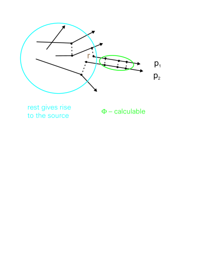
Figure 1: Separation of the interference and final-state interactions, in terms of the two-particle wavefunction, from the amplitude for the reaction.

The rest of the amplitude squared, integrated in the cross section over unobserved particles, yields the unnormalized Wigner function $S^{\prime}$ for the distribution of emission points written here in the two-particle frame:

$${d^{6}\sigma\over d^{3}{p}_{1}\,d^{3}{p}_{2}}=\int d^{3}{r}\,S^{\prime}_{\vec{P}}(\vec{r})\,|\Phi_{\vec{p}_{1}-\vec{p}_{2}}^{(-)}(\vec{r})|^{2}\,.$$ (2)

The vector $\vec{r}$ is the relative separation between emission points and the equation refers to the case of particles with equal masses. The size of the source $S^{\prime}$ is of the order of the spatial extent of reaction. The possibility of probing structures of this size arises when the wave-function modulus squared, $|\Phi^{(-)}|^{2}$, possesses pronounced structures, either due to interaction or symmetrization, that vary rapidly with the relative momentum, typically at low momenta. The two-particle cross section can be normalized to the single-particle cross sections to yield the correlation function $C$:

$$C(\vec{p}_{1}-\vec{p}_{2})={{d^{6}\sigma\over d^{3}{p}_{1}\,d^{3}{p}_{2}}\over{d^{3}\sigma\over d^{3}{p}_{1}}\,{d^{3}\sigma\over d^{3}{p}_{2}}}=\int d^{3}{r}\,S_{\vec{P}}(\vec{r})\,|\Phi_{\vec{p}_{1}-\vec{p}_{2}}^{(-)}(\vec{r})|^{2}\,.$$ (3)

The source $S$ is normalized to 1 as, for large relative momenta, $C$ is close to 1 and $|\Phi|^{2}$ in (3) averages to 1:

$$\int d^{3}{r}\,S_{\vec{P}}(\vec{r})=1\,.$$ (4)

Depending on how the particles are emitted from a reaction, the source may have different features. For a prompt emission, we expect the source to be compact and generally isotropic. In the case of prolonged emission, we expect the source to be elongated along the pair momentum, as the emitting system moves in the two-particle cm. Finally, in the case of secondary decays, we expect the source may have an extended tail.

In the following, I shall discuss restoring the sources in heavy-ion reactions and extracting information from the images [2].

2 Imaging in the Reactions

The interesting part of the correlation function is its deviation from 1 so we rewrite (3)

$${\cal R}_{\vec{P}}(\vec{q})=C_{\vec{P}}(\vec{q})-1 = \int{d}^{3}r\>\left(\left|\Phi^{(-)}_{\vec{{q}}}(\vec{{r}})\right|^{2}-1\right)S_{\vec{P}}(\vec{r})$$ (5)

$$= \int{d}^{3}r\>K(\vec{q},\vec{r})\,S_{\vec{P}}(\vec{r})\,.$$

From (5), it is apparent that to make the imaging possible $\left|\Phi^{(-)}_{\vec{q}}(\vec{r})\right|^{2}$ must deviate from 1 either on account of symmetrization or interaction within the pair. The angle-averaged version of (5) is

$${\cal R}_{P}({q})=4\pi\int dr\,r^{2}\,K_{0}({q},{r})\,S^{0}_{P}(r)$$ (6)

where $K_{0}$ is the angle-averaged kernel.

Let us first take the case of identical bosons with negligible interaction, such as neutral pions or gammas. The two-particle wavefunction is then

$$\Phi^{(-)}_{\vec{q}}(\vec{r})=\frac{1}{\sqrt{2}}\left(e^{i\vec{q}\cdot\vec{r}}+e^{-i\vec{q}\cdot\vec{r}}\right)\,.$$ (7)

The interference term causes $\left|\Phi^{(-)}_{\vec{q}}(\vec{r})\right|^{2}$ to deviate from 1 and

$$K(\vec{q},\vec{r})=\cos{(2\vec{q}\cdot\vec{r})}.$$ (8)

In this case, the source is an inverse Fourier cosine-transform of ${\cal R}_{P}$. Also, the angle averaged source can be determined from a Fourier transformation (FT) of the angle-averaged $C$ as the averaged kernel is

$$K^{0}(q,r)=\frac{\sin{(2qr)}}{2qr}\,.$$ (9)

While neutral pion and gamma correlations functions are difficult to measure, charged pion correlations functions are not. The charged pion correlations are often corrected approximately for the pion Coulomb interactions allowing for the use of FT in the pion source determination. In Figure 2, I show one such corrected correlation function for negative pions from the Au + Au reaction at 10.8 GeV/nucleon from the measurements by E877 collaboration at AGS [3].

Figure 2: Gamow-corrected $\pi^{-}\pi^{-}$ correlation function for Au + Au reaction at 10.8 GeV/nucleon obtained by the E877 collaboration [3].

In Figure 3, I show the relative distribution of emission points for negative pions obtained through the FT of the correlation function in Fig. 2.

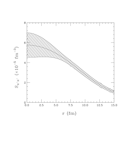
Figure 3: Relative source function for negative pions from FT of the correlation function in Fig. 2.

The FT has been cut off at $q_{max}=200~{}MeV/c$ giving a resolution in the source of $\Delta r\raisebox{-2.15277pt}{$\,\stackrel{{\scriptstyle>}}{{\scriptstyle\sim}}\,$}1/(2\,q_{max})=2.0$ fm. The data spacing gives the highest distances that can be studied with FT of $r_{max}\raisebox{-2.15277pt}{$\,\stackrel{{\scriptstyle<}}{{\scriptstyle\sim}}\,$}1/(2\,\Delta q)=20$ fm. As you see, the relative source has a roughly Gaussian shape.

3 Perils of Inversion

For many particle pairs, such as proton pairs, interactions cannot be ignored and the straightforward FT cannot be used. Indeed, even in the charged-pion case, one might want to avoid the approximate Coulomb correction. In lieu of this, we can simply discretize the source and find the source that minimizes the $\chi^{2}$. This procedure could work for any particle pair.

With measurements of $C$ at relative momenta $\{q_{i}\}$ and assuming the source is constant over intervals $\{\Delta r_{j}\}$, we can write Eq. (6) as

$${\cal R}_{i}=C_{00}(q_{i})-1 = \sum_{j}4\pi\,\Delta r\,r_{j}^{2}\,K_{0}(q_{i},r_{j})\,S(r_{j})$$ (10)

$$\equiv \sum_{j}K_{ij}\,S_{j}\,.$$ (11)

The values ${S_{j}}$ can be varied to minimize the $\chi^{2}$:

$$\chi^{2}=\sum_{j}\frac{({\cal R}^{th}(q_{j})-{\cal R}^{exp}(q_{j}))^{2}}{\sigma_{j}^{2}}\,.$$ (12)

Derivatives of the $\chi^{2}$ with respect to $S$ give linear algebraic eqs. for $S$:

$$\sum_{ij}{1\over\sigma_{i}^{2}}(K_{ij}\,S_{j}-{\cal R}_{i}^{exp})\,K_{ij}=0\,,$$ (13)

with the solution in a schematic matrix form:

$$S=(K^{\top}K)^{-1}\,K^{\top}\,{\cal R}^{exp}\,.$$ (14)

There is an issue in the above: how do we discretize the source? The FT used before suggests fixed-size bins, e.g. $\Delta r=2$ fm. However fixed size bins may not be ideal for all situations as I will illustrate using Fig. 4. This figure shows the $pp$ correlation function from the measurements [4] of the ¹⁴N + ²⁷Al reaction at 75 MeV/nucleon, in different intervals of total pair momentum.

Figure 4: Two-proton correlation function for the ¹⁴N + ²⁷Al reaction at 75 MeV/nucleon from the measurements of Ref. [4] for three gates of total momentum imposed on protons emitted in the vicinity of $\theta_{\rm lab}=25^{\circ}$.

The different regions in relative momentum are associated with different physics of the correlation function. For example, the peak around $q\sim 20$ MeV/c is associated with the ${}^{1}S_{0}$ resonance of the wavefunction with a characteristic scale of fm – this gives access to a short range structure of the source. On the other hand, the decline in the correlation function at low momenta is associated with the Coulomb repulsion that dominates at large proton separation and gives access to the source up to (20–30) fm or more, depending on how low momenta are available for $C$. Should we continue at the resolution of $\Delta r\raisebox{-2.15277pt}{$\,\stackrel{{\scriptstyle>}}{{\scriptstyle\sim}}\,$}2$ fm up to such distances? No! At some point there would not be enough many data points to determine the required number of source values! Somehow, we should let the resolution vary, depending on the scale at which we look.

A further issue is that the errors on the source may explode in certain cases. The errors are given by the inverse square of the kernel:

$$\Delta^{2}S_{j}=(K^{\top}\,K)^{-1}_{jj}\,.$$ (15)

The square of the kernel may be diagonalized:

$$(K^{\top}\,K)_{ij}\equiv\sum_{k}{1\over\sigma_{k}^{2}}K_{ki}\,K_{kj}=\sum_{\alpha}\lambda_{\alpha}\,u_{i}^{\alpha}\,u_{j}^{\alpha}\,.$$ (16)

where $\{u^{\alpha}\}$ are orthonormal and $\lambda_{\alpha}\geq 0$; the number of vectors of equals the number of $r$ pts. The errors can be expressed as

$$\Delta^{2}S_{j}=\sum_{\alpha}{1\over\lambda_{\alpha}}\,u_{j}^{\alpha}\,u_{j}^{\alpha}\,.$$ (17)

You can see from the last equation that the errors blow up, and inversion problem becomes unstable, if one or more $\lambda$’s approach zero. This must happen when $K$ maps a region to zero (remember $K=|\Phi|^{2}-1$), or when $K$ is too smooth and/or too high resolution is demanded. A $\lambda$ close to 0 may be also hit by accident.

The stability issue is illustrated with Figs. 5 and 6. Figure 5 shows correlation functions from model sources with small errors added on.

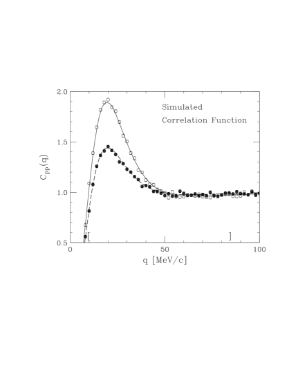
Figure 5: The solid line represents the correlation function from a Gaussian model source while the dashed lines represent the correlation functions from a source with an extended tail. The points represent values of $C$ with errors that are typical for the measurements in Ref. [4] (Fig. 4).

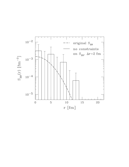
Figure 6: The solid histogram is the relative $pp$ source function $S$ restored from the simulated correlation function in Fig. 5 from the Gaussian model source (open symbols there). The dashed line is the original source function that we used to generate the correlation function. We employed fixed-size intervals of $\Delta r=2$ fm and we imposed no constraints on $S$.

Figure 6 shows the source in 7 fixed-size intervals of $\Delta r=2$ fm. This source was restored following Eq. (14), from the correlation function indicated in Fig. 5. The errors in this case far exceed the original source function. Every second value of the restored source is negative.

Vast literature, extending back nearly 75 years, exists on stability in inversion. One of the first researchers to recognize the difficulty, Hadamard, in 1923 [5], argued that the potentially unstable problems should not be tackled. A major step forward was made by Tikhonov [6] who has shown that placing constraints on the solution can have a dramatic stabilizing effect. In determining the source from data, we developed a method of optimized discretization for the source which yields stable results even without any constraints [2].

In our method, we first concentrate on the errors. We use the $q$-values for which the correlation function is determined and the errors of $\{\sigma_{i}\}$, but we disregard the values $\{C_{i}\}$. We optimize the binning for the source function to minimize expected errors relative to a rough guess on the source $S^{mod}$:

$$\sum_{j}{\Delta S_{j}\over S_{j}^{mod}}=\sum_{j}{1\over S_{j}^{mod}}\left(\sum_{\alpha}{1\over\lambda_{\alpha}}\,u_{j}^{\alpha}\,u_{j}^{\alpha}\right)^{1/2}\,.$$ (18)

Only afterwards we use $\{C_{i}\}$ to determine source values $S_{j}$ with the optimized binning. This consistently yields small errors and an introduction of constraints may additionally reduce those errors. The proton source imaged using the optimized binning from the correlation function in Fig. 5 is shown in Fig. 7.

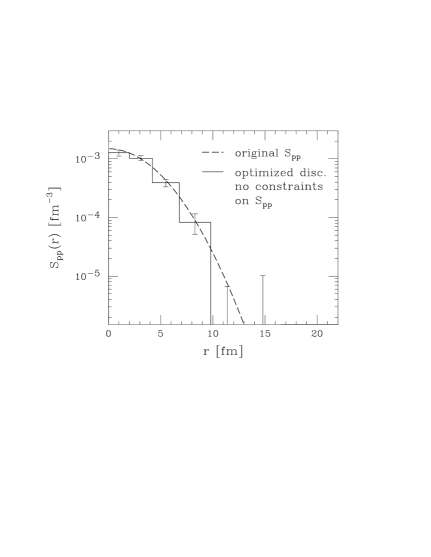
Figure 7: Relative pp source function $S$ restored (solid histogram) through the optimized discretization from the correlation function in Fig. 5 (open symbols there), together with the original source function (dashed line).

4 pp Sources

Upon testing the method, we apply it to the 75 MeV/nucleon ¹⁴N + ²⁷Al data by Gong et al. [4] shown in Fig. 4. In terms of the radial wavefunctions $g$, the angle-averaged $pp$ kernel is

$$K_{0}(q,r)=\frac{1}{2}\sum_{js\ell\ell^{\prime}}(2j+1)(g_{js}^{jj^{\prime}}(r))^{2}-1\,.$$ (19)

We calculate the wavefunctions by solving radial Schrödinger equations with REID93 [7] and Coulomb potentials. The sources restored in the three total momentum intervals are shown in Fig. 8, together with sources obtained directly from a Boltzmann equation model [8] (BEM) for heavy-ion reactions.

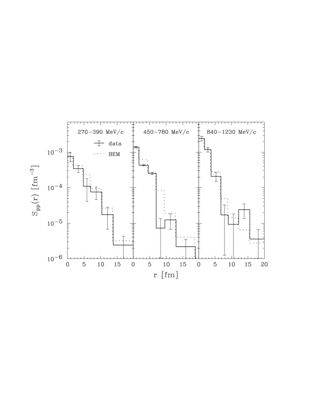
Figure 8: Relative source for protons emitted from the ¹⁴N + ²⁷Al reaction at 75 MeV/nucleon, in the vicinity of $\theta_{\rm lab}=25^{\circ}$, within three intervals of total momentum of 270–390 MeV/c (left panel), 450–780 MeV/c (center panel), and 840–1230 MeV/c (right panel). Solid and dotted lines indicate, respectively, the source values extracted from data [4] and obtained within the Boltzmann-equation calculation.

The sources become more focussed around $r=0$ as total momentum increases. Now, the value of the source as $r\rightarrow 0$ gives information on the average density at freeze-out, on space-averaged phase-space density, and on the entropy per nucleon. The freeze-out density may be estimated from

$$\rho_{freeze}\simeq N_{\rm part}\times S(r\rightarrow 0)\,,$$ (20)

where $N_{\rm part}$ is participant multiplicity. Using the intermediate momentum range, we find

$$\rho_{freeze}\approx(17)(.0015{\rm fm}^{-3})=.16\rho_{0}\,.$$ (21)

The space–averaged phase-space density may be estimated from

$$f(\vec{p})\approx\frac{(2\pi)^{3}}{2s+1}\frac{dN_{1}}{d\vec{P}}S_{\vec{P}}({r}\rightarrow 0)\,.$$ (22)

Using the intermediate momentum range we get $\langle f\rangle\approx.23$ for this reaction.

The transport model reproduces the low-$r$ features of the sources, including the increased focusing as the total momentum increases. The average freeze-out density obtained directly within the model is $\rho_{freeze}\simeq.14\rho_{0}$. Despite the agreement at low $r$ between the data and the model, we see important discrepancies at large $r$. I discuss these next.

An important quantity characterizing images is the portion of the source below a certain distance (e.g. the maximum $r$ imaged):

$$\lambda(r_{max})=\int_{r<r_{max}}d^{3}r\,S(\vec{r})\,.$$ (23)

If $r_{max}\Rightarrow\infty$, then $\lambda$ approaches unity. The value of $\lambda<1$ signals that some of the strength of $S$ lies outside of the imaged region. The imaged region is limited in practice by the available information on details of $C$ at very-low $q$. We can expect pronounced effects for secondary decays or for long source lifetimes. If some particles stem from decays of long-lived resonances, they may be emitted far from any other particles and contribute to $S$ at $r>r_{max}$.

Table 1 gives the integrals of the imaged sources together with the integrals of the sources from BEM over the same spatial region.

$P$-Range	$\lambda(r_{max})$			$r_{max}$
[MeV/c]	restored		BEM	[fm]
270-390	0.69$\pm$	0.15	0.98	20.0
450-780	0.574$\pm$	0.053	0.91	18.8
840-1230	0.87$\pm$	0.14	0.88	20.8

Table 1: Integrals of sources from data and BEM in the three intervals of total momentum.

Significant strength is missing from the imaged sources in the low and intermediate momentum intervals. BEM agrees with data in the highest momentum interval but not in the two lower-momentum intervals. In BEM there is no intermediate mass fragment (IMF) production. The IMFs might be produced in excited states and, by decaying, contribute protons with low momenta spread out over large spatial distances. Information on this possibility can be obtained by examining the IMF correlation functions.

5 IMF Sources

Because of the large charges ($Z\geq 3$), the kernel in the case of IMFs is dominated by Coulomb repulsion. With many partial waves contributing, the kernel approaches the classical limit [9]:

$$K_{0}(q,r)=\theta(r-r_{c})(1-r_{c}/r)^{1/2}-1\,,$$ (24)

where $r_{c}=2\mu Z_{1}Z_{2}e^{2}/q^{2}$ is the distance of closest approach. There are no IMF correlation data available for the same reaction used to measure the pp correlation data, so we use data within the same beam energy range, i.e. the ${}^{84}Kr-^{197}Au$ at 35, 55, and 70 MeV/nucleon data by Hamilton et al. [10]. The extracted relative IMF sources are shown in Fig. 9.

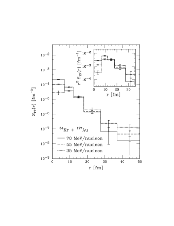
Figure 9: Relative source for IMFs emitted from central ⁸⁴Kr + ¹⁹⁷Au reactions from the data of Ref. [10] at 35 (dotted line), 55 (dashed line), and 70 MeV/nucleon (solid line). The insert shows the source multiplied by $r^{2}$. In both plots, the full image extends out to $90$ fm.

The source integrals for the IMF sources are given in Table 2. Interestingly, we are nearly capable of restoring the complete IMF sources.

Beam Energy	$\lambda(90\,{\rm fm})$		$\lambda(20\,{\rm fm})$
[MeV/A]
35	0.96$\pm$	0.07	0.72$\pm$	0.04
55	0.97$\pm$	0.06	0.78$\pm$	0.03
70	0.99$\pm$	0.05	0.79$\pm$	0.03

Table 2: Comparison of the integrals of the midrapidity IMF source function, $\lambda(r_{max})$, in central ⁸⁴Kr + ¹⁹⁷Au reactions at three beam energies, for different truncation points, $r_{max}$. The restored sources use the data of Ref. [10].

For the relative distances that are accessible using the pp correlations ($\sim 20$ fm) we find only (70–80)% of the IMF sources. This is is comparable to what we see for the lowest-momentum pp source but above the intermediate-momentum proton source. We should mention that we can not expect complete quantitative agreement, even if the data were from the same reaction and pertained to the same particle-velocity range. This is due partly to the fact that more protons than final IMFs can stem from secondary decays.

6 $\pi^{-}$ vs. $K^{+}$ Sources

We end our discussion of imaging by presenting sources obtained for pions and kaons from central Au + Au reactions at about 11 GeV/nucleon. This time we use the optimized discretization technique rather than the combination of approximate Coulomb corrections and the FT. For both meson pairs the kernel $K_{0}$ is given by a sum over partial waves:

$$K_{0}(q,r)=\sum_{\ell}\frac{(g^{\ell}(r))^{2}}{(2\ell+1)}-1.$$ (25)

where $g_{\ell}(r)$s stem from solving the radial Klein-Gordon equation with strong and Coulomb interactions. In practice the strong interactions had barely any effect on the kernels and the extracted sources.

The data come from the reactions at 10.8 and 11.4 GeV/nucleon [3]. The respective $\pi^{-}$ and $K^{+}$ sources are displayed Fig. 10.

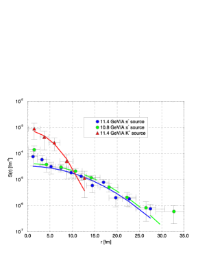
Figure 10: Relative sources of $\pi^{-}$ (circles) and of $K^{+}$ (triangles) extracted from central Au + Au data at 11.4 GeV/nucleon [11], for $\pi^{-}$ and $K^{+}$, and at 10.8 GeV/nucleon [3], for $\pi^{-}$. Lines show Gaussian fits to the sources.

The kaon source is far more compact than the pion source and there are several effects that contribute to this difference. First, kaons have lower scattering cross sections than pions, making it easier for kaons to leave the system early. Second, fewer kaons than pions descend from long-lived resonances. Next, due to their higher mass, the average kaon has a lower speed than the average pion, making the kaons less sensitive to lifetime effects. Finally, the kaons are more sensitive to collective motion than pions, enhancing the kaons’ space-momentum correlations. Differences, qualitatively similar to those seen in Fig. 10, in the spatial distributions of emission points for kaons and pions were predicted long ago within RQMD by Sullivan et al. [12]. In the model, they were able to separate the different contributions to the source functions.

The effects of long-lived resonances, mentioned above, are apparent in the sources extracted from the data. Thus, Table 3 gives

	$R_{0}$ [fm]	$\bar{\lambda}$	$\lambda(35{\rm fm})$
$K^{+}$ (11.4 GeV/A)	2.76	0.702	0.86$\pm$	0.56
$\pi^{-}$ (11.4 GeV/A)	6.42	0.384	0.44$\pm$	0.17
$\pi^{-}$ (10.8 GeV/A)	6.43	0.486	0.59$\pm$	0.22

Table 3: Parameters of Gaussian fits to the sources and integrals over imaged regions for the central Au + Au reactions.

the source integrals over the imaged regions together with parameters of the Gaussian fits to the sources,

$$S(r)=\frac{\bar{\lambda}}{(2\sqrt{\pi}R_{0})^{3}}\exp{\left(-\left(\frac{r}{2R_{0}}\right)^{2}\right)}\,.$$ (26)

The errors are quite small for the fitted values. We find $\bar{\lambda}_{\pi^{-}}<\bar{\lambda}_{K^{+}}<1$ and $\bar{\lambda}\raisebox{-2.15277pt}{$\,\stackrel{{\scriptstyle<}}{{\scriptstyle\sim}}\,$}\lambda$.

7 Conclusions

We have demonstrated that a model-independent imaging of reactions is possible. Specifically, we have carried out one-dimensional imaging of pion, kaon, proton, and IMF sources. The three-dimensional imaging of pion sources is in progress. Our method of optimized discretization allows us to investigate the sources on a logarithmic scale up to large distances. The sources generally contain information on freeze-out phase-space density, entropy, spatial density, lifetime and size of the freeze-out region, as well as on resonance decays. The imaging gives us access to the spatial structure required to extract that information.

References

References

- [1] D. H. Boal, C. K. Gelbke, and B. K. Jennings, Rev. Mod. Phys. 62, 553 (1990).
- [2] D. A. Brown and P. Danielewicz, Phys. Lett. B 398, 252 (1997); Phys. Rev. C 57, 2474 (1998).
- [3] J. Barette et al., Phys. Rev. Lett. 78, 2916 (1997).
- [4] W. G. Gong et al., Phys. Rev. C 43, 1804 (1991).
- [5] J. Hadamard, Lectures on the Cauchy Problem in Linear Partial Differential Equations (Yale U. Press, New Haven, 1923).
- [6] A. N. Tikhonov, Sov. Math. Dokl. 4, 1035 (1963).
- [7] V. G. J. Stoks et al., Phys. Rev. C 49, 2950 (1994).
- [8] P. Danielewicz, Phys. Rev. C 51, 716 (1995).
- [9] Y. D. Kim et al., Phys. Rev. Lett. 67, 14 (1991).
- [10] T. M. Hamilton et al., Phys. Rev. C 53, 2273 (1996).
- [11] T. Vongpaseuth et al., Czech. J. of Phys. Suppl. S1, 48 (1998).
- [12] J. Sullivan et al., Phys. Rev. Lett. 93, 3000 (1993).