Numerical studies of left-handed materials and arrays of split ring resonators.

Abstract

We present numerical results on the transmission properties of the left-handed materials (LHM) and split-ring resonators (SRR). The simulation results are in qualitative agreement with experiments. The dependence of the transmission through LHM on the real and imaginary part of the electric permittivity of the metal, the length of the system, and the size of the unit cell are presented. We also study the dependence of the resonance frequency of the array of SRR on the ring thickness, inner diameter, radial and azimuthal gap, as well as on the electrical permittivity of the board and the embedding medium, where SRR resides. Qualitatively good agreement with previously published analytical results is obtained.

PACS numbers: 73.20.Mf,41.20.Jb,42.70Qs

I Introduction

Very recently, a new area of the research, called left-handed materials (LHM) has been experimentally demonstrated by Smith et al. [3, 4] based on the work of Pendry et al. [5, 6]. LHM are by definition composites, whose properties are not determined by the fundamental physical properties of their constituents but by the shape and distribution of specific patterns included in them. Thus, for certain patterns and distribution, the measured effective permittivity $\epsilon_{\rm eff}$ and the effective permeability $\mu_{\rm eff}$ can be made to be less than zero. In such materials, the phase and group velocity of an electro-magnetic wave propagate in opposite directions giving rise to a number of novel properties [7]. This behavior has been called “left-handedness”, a term first used by Veselago [8] over thirty years ago, to describe the fact that the electric field, magnetic intensity and propagation vector are related by a left-handed rule.

By combining a 2D array of split-ring resonators (SRRs) with a 2D array of wires, Smith et al. [3] demonstrated for the first time the existence of left-handed materials. Pendry et al. [6] has suggested that an array of SRRs give an effective $\mu_{\rm eff}$, which can be negative close to its resonance frequency. It is also well known [5, 9] that an array of metallic wires behaves like a high-pass filter, which means that the effective dielectric constant is negative at low frequencies. Recently, Shelby et al. [10] demonstrated experimentally that the index of refraction $n$ is negative for a LHM. Negative refraction index was obtained analytically[11] and also from numerically simulated data [12]. Also, Pendry [13] has suggested that a LHM with negative $n$ can make a perfect lens.

Specific properties of LHM makes them interesting for physical and technological applications. While experimental preparation of the LHM structures is rather difficult, especially when isotropic structures are required, numerical simulations could predict how the transmission properties depends on various structural parameters of the system. It will be extremely difficult, if not impossible, to predict the transmission properties of such materials analytically. Mutual electro-magnetic interaction of neighboring SRRs and wires makes the problem even more difficult. Numerical simulations of various configurations of SRRs and of LHMs could be therefore very useful in searching of the direction of the technological development.

In this paper, we present systematic numerical results for the transmission properties of LHMs and SRRs. An improved version of the transfer-matrix method (TMM) is used. Transfer matrix was applied to problems of the transmission of the electro-magnetic (EM) waves through non-homogeneous media many years ago [14, 15, 16]. It was also used in numerical simulations of the photonic band gap materials (for references see Ref. 15). TMM enables us to find a transmission and a reflection matrices from which the transmission, reflection and absorption could be obtained. The original numerical algorithm was described in Ref. 13. In our program we use a different algorithm which was originally developed for the calculation of the electronic conductance of disordered solids [18].

The paper is organized as follows: In Section II we describe briefly the structure. We concentrate on the structure displayed in Figure 1. In Section III we present and discuss our results. The dependence of the transmission of the LHM and SRR on the electrical permittivity of the metallic components of our structure is given in Section III A. In Section III B we present the dependence of the transmission of the LHM on the size of the unit cell and size of the metallic wires. In Section III C we show the dependence of the resonance frequency of SRR on the parameters of the SRR. Section III D deals with the dependence of the resonance frequency on the permittivity of the board and embedding media. In Section IV we summarize our results and give some conclusions. Finally, in the Appendix A we give detailed description of the transfer matrix method.

II Structure of the LHM meta-material

Both in the experiment and in the numerical simulations, the left-handed meta-materials consist from an array of unit cells, each containing one SRR and one wire. Figure 1a shows a realization of the unit cell that we have simulated. The size of the unit cell $L_{x}\times L_{y}\times L_{z}$ and the size of SRR itself are of order of mm. Waves propagate along the $z$-direction. The SRR lies in the $yz$ plane, and the wire is parallel to the $y$ axis.

As we are interested mostly in the transmission properties of the left-handed meta-material, the configuration as presented in Figure 1a, should be considered as one-dimensional. Indeed, such meta-materials possesses the left-handed properties only for the electro-magnetic wave incoming in the $z$-direction and even then only for a given polarization. Two-dimensional structures have been realized in experiments [4, 10], in which two SRRs have been positioned in each unit cell in two perpendicular planes. For such structures, left-handed transmission properties have been observed for waves coming from any direction in the $xz$ plane. No three - dimensional structure has been realized so far.

Figure 1b shows a single square SRR of the type used for our simulations and also for experiments [4]. The structure of the SRR is defined by the following parameters: the ring thickness $c$, the radial gap $d$, the azimuthal gap $g$ and the inner diameter $r$. The size of the SRR is

$$w=4c+2d+r.$$ (1)

Another parameter is the thickness of the SRR itself (in the $x$-direction). This thickness is very small in the experiments ($\sim 0.02$ mm). We can not simulate such thin structures yet. In numerical simulations, we divide the unit cell into $N_{x}\times N_{y}\times N_{z}$ mesh points. For homogeneous discretization, used throughout this paper, the discretization defines the minimum unit length $\delta=L_{x}/N_{x}$. All length parameters are then given as integer of $\delta$. This holds also for the thickness of the SRR. Generally, the thickness of SRR used in our simulations is 0.25-0.33 mm. Although we do not expect that the thickness will considerably influence the electro-magnetic properties of the SRR, it still could cause small quantitative difference between our data and the experimental results.

III Structural parameters

A Metallic permittivity

The existence of LHM has been experimentally demonstrated [3, 4] for structures that have resonance frequencies in the GHz region. In this frequency region, we do not know the exact values of electrical permittivity $\epsilon_{\rm m}$ of the metal. We know that Im $\epsilon_{\rm m}$ is very large, and/or the Re $\epsilon_{\rm m}$ is large but negative. In our previous studies [19] we have found that the resonance frequency $\nu_{0}$ of the LHM depends only on the absolute value of $\epsilon_{\rm m}$. In fact $\nu_{0}$ reaches the saturated value provided that $|\epsilon_{\rm m}|>10^{4}$. Since we do not know the exact values of the metallic permittivity, we have studied the transmission of the LHM with different values of $\epsilon_{\rm m}$. In the results presented in Figure 2, we choose $\epsilon_{\rm m}=1+i~{}{\rm Im}~{}\epsilon_{\rm m}$ with different values of Im $\epsilon_{\rm m}$. [20] The last is proportional to $\sigma(\omega)/\omega$ [21]. For simplicity, we neglect the $\omega$-dependence of Im $\epsilon_{\rm m}$ and consider Im $\epsilon_{\rm m}$ = 8000, 18000 and 38000 for the three cases presented in Figure 2. For each case, we present results of transmission for different number (1 to 10) of unit cells. Notice that the higher imaginary part of the metal the higher is the transmission. Also the losses due to the absorption are smaller, as can be seen from the decrease of the transmission peak as the length of the system increases. This result is consistent with the formula presented by Pendry et al. [6] for the effective permeability of the system

$$\mu_{\rm eff}=1-\frac{F\nu^{2}}{\nu^{2}-\nu_{0}^{2}+i\gamma\nu}$$ (2)

with the damping factor

$$2\pi\gamma=\frac{2L_{x}\rho}{r\mu_{0}}$$ (3)

and the resonance frequency

$$(2\pi\nu_{0})^{2}=\frac{3L_{x}c_{\rm light}^{2}}{\pi\ln\left(\frac{2c}{d}\right)r^{3}}.$$ (4)

where $\rho$ is the resistance of the metal, $L_{x}$ is the size of the system along the $x$ axis, $c_{\rm light}$ is a the velocity of light in vacuum and parameters $r$, $c$ and $d$ characterize the structure of SRR. They are defined in Figure 1b. Notice that the damping term $\gamma\to 0$ as $\sigma\to\infty$. Since the Im $\epsilon_{\rm m}$ is proportional to $\sigma$, $\gamma$ is inversely proportional to Im $\epsilon_{\rm m}$. Our numerical results suggest that it is reasonable to expect that the LHM effect will be more pronounced in systems with higher conductivity.

In Figure 3, we present the frequency dependence of the transmission for SRRs with the same parameters as those in Figure 2. Notice that the transmission is more pronounced as the length of the system is increased. Note also that the resonance gap becomes narrower when Im $\epsilon_{\rm m}$ increases. This is in agreement with Eq. (2). The frequency interval, in which the effective permeability is negative, becomes narrower when the damping factor $\gamma$ decreases.

In Figure 4 we show the transmission through the LHM, in which the SRR are turned around their axis by 90 degrees. If we keep the same size of the unit cell as that of Figure 2, we do not obtain any LHM peak in the transmission, although there is a very well defined gap for the SRR alone. It seems that for this orientation of the SRR there is no overlap of the field of the wire with that of the SRR. The results shown in Figures 4 and 5 are therefore obtained with a reduced unit cell of $3.66\times 3.66\times 3.66$ mm (the size of SRR is still $3\times 3$ mm). The LHM transmission peak is located close to the lower edge of the SRR gap (shown in Figure 5). This is in contrast to the results presented in Figures 2 and 3, where the LHM transmission peak is always located close to the upper edge of the SRR gap. Finally, the gap shown for the “turned” SRR shown in the Figure 5, is deeper and broader than the gap for the “up” SRR.

In fact, for the SRR “up” structure, we found that the transmission in the gap is always of order of $10^{-7}-10^{-8}$. We can explain this effect by non-zero transmission from the $p$ to $s$ polarized wave (and back). If the transmission $t(p\to s)$ and $t(s\to p)>0$, then there is always the non-zero probability $\propto t(p\to s)t(s\to p)$ for the $p$-polarized wave to switch into the $s$ state, at the beginning of the sample, move throughout the sample as the $s$ wave (for which neither wires nor SRR are interesting), and in the last unit cell to switch back into the $p$-polarized state. This process contributes to the transmission probability $T(p\to p)$ of the whole sample and determines the bottom level of the transmission gap for SRR. We indeed found that $t(s\to p)\sim 10^{-4}$ for the “up” SRR. In the “turned” SRR case, both $t(p\to s)$ and $t(s\to p)$ should be zero due to the symmetry of the unit cell.[22] Our data give $t(p\to s)\sim t(s\to p)\sim 10^{-6}$ for the “turned” SRR which determines the decrease of the transmission in the gap below $10^{-11}$.

B Dependence on the size of the unit cell and the width of the metallic wire.

As we discussed in Section III A, the transmission peak for the LHM with cuts in the SRR in the horizontal direction appears only when the size of the unit cell is really small. The effect of the size of the unit cell was demonstrated already in Figures 2 and 3, where we compared the transmission for the “up” SRR and LHM of different size of the unit cell. Both the transmission gap for an array of SRRs and the transmission peak for LHM are broader for smaller unit cell.

In Figure 6, we show the transmission for the LHM structure with q unit cell of size $5\times 3.66\times 5$ mm for the “turned” SRR. Evidently, there is no transmission peak for all the system lengths studied. The size of the unit cell must be reduced considerably to obtain a transmission peak.

Figure 7 presents the transmission peak for various sizes of the unit cell. Resonance frequency decreases as the distance between the SRRs in the $x$ direction decreases. This agree qualitatively (although not quantitatively) with theoretical formula given by Eqn. (4). We see also that an increase of the distance between SRR in the $z$ direction while keeping the $L_{x}$ constant causes sharp decrease and narrowness of the transmission peak.

C Resonance frequency of SRR

In this section we study how the structure of the SRR influences the position of the resonance gap. In order to simulate various forms of the SRR, we need to have as many as possible mesh points in the $yz$ plane. Keeping in mind the increase of the computer time when the number of mesh points increases, we used a unit cell with $L_{x}<L_{y},L_{z}$. The actual size of the unit cell in this section is $L_{x}=2.63$ mm and $L_{y}=L_{z}=6.05$ mm. and we use uniform discretization with $N_{x}\times N_{y}\times N_{z}=10\times 23\times 23$ mesh points. This discretization defines a minimum unit length $\delta=0.263$ mm. SRR with size of $\approx 5\times 5$ mm, is divided into $19\times 19$ mesh points.

The electrical permittivity of the metallic components is chosen to be $\epsilon_{\rm m}=-1000+10.000~{}i$. We expect that larger value of Im $\epsilon_{\rm m}$ will increase a little the position of the resonance gap [19]. However, the dependence on the different structural parameters will remain the same. Higher values of $|\epsilon_{\rm m}|$, however, will require more CPU time because of shorter interval between the normalization of the transmitted waves (see Appendix A for details).

We have considered 23 different SRR structures and studied how the resonance frequency $\nu_{0}$ depends on the structure parameters. The lowest $\nu_{0}=3.75$ GHz was found for SRR with c : d : r : g = 1 : 1 : 13 : 1. On the other hand, SRR with c : d : r : g = 2 : 3 : 5 : 3 exhibits $\nu_{0}=6.86$ GHz.

We present our results on the dependence of $\nu_{0}$ on the azimuthal gap $c$ (Figure 8), radial gap $g$ (Figure 9) and ring thickness $d$ (Figure 10). In all these cases $\nu_{0}$ increases as the different parameters increase. The dependence shown in Figures 8-10 agrees qualitatively with those done by a different numerical method [23]. When compare our results with the analytical arguments presented by Pendry et al. [6], we have to keep in mind that that various assumptions about the structural parameters have been done in derivation of Eqn. (4), which are not fulfilled for our structure. Note also that the azimuthal gap does not enter the formula for the resonance frequency given by Eq. (4). Moreover, as the size of the SRR is constant, the structural parameters are not independent each form other. Thus, due to the Eq. (1), increase of the azimuthal gap causes decrease of the inner diameter and vice versa. When taking these restrictions into account, the agreement with analytical results is satisfactory.

D Material parameters

In Figures 11 and 12 we show how the resonance frequency depends on the permittivity of the dielectric board and on the permittivity of the embedding media. As expected, the resonance frequency decreases considerably with the increase of the value of both permittivities.

IV Conclusion

In summary, we have used the transfer matrix method to calculate the transmission properties of the left-handed materials and arrays of split ring resonators. The role of absorption of the metallic components of our SRR and LHM has been simulated. It is found that the LHM transmission peak depends on the imaginary part of the metallic permittivity $\epsilon_{\rm m}$, the length of the system and the size of the unit cell. Higher conductivity of the metal guarantees better transmission properties of LHM.

For an array of SRR, the resonance frequency $\nu_{0}$ was computed and is found to agree with experimental data. The dependence of the resonance frequency $\nu_{0}$ on various structural parameters of the SRR were numerically obtained and compared with analytical estimates and also with other numerical techniques.

The main disadvantage of the presented transfer-matrix method is that it can not treat structures with smaller length scales than our discretization mesh. For example, the thickness of the SRR is an order of magnitude smaller in experiments than in our simulation. Also structural parameters of SRR can be changed only discontinuously as multiplies of the unit mesh length. This could be partially overcomed by generalizing the present code to a non-uniform mesh discretization. Nevertheless, already uniform discretization enables us to obtain credible data. Comparison of our results with those obtained by the commercial software MAFIA [24] confirmed that both methods find the same position of the resonant gap provided that they use the same mesh discretization.

Our numerical data agree qualitatively with the experimental results. [3] As we can not tune the exact parameters of SRR (as well as its circular shape), and when taken into account the strong dependence of the resonance frequency on the permittivity of the board, we do not expect to obtain very accurate quantitative agreement with experimental data.

Our studies demonstrate that the transfer matrix method can be reliable used to calculate the transmission and reflection properties of left-handed materials and split-ring resonators. Thus, numerical simulations could answer some practical questions about different proposed structures, which might be too complicated to be treated by analytical studies. The transfer matrix method can be used in the future for detailed studies of two-dimensional and even three-dimensional structures. These structures should contain more SRRs and wires per unit cell, which makes their analytical analysis extremely difficult. On the other hand, it is extremely important to find the best design and test the transmission properties of proposed meta-material even before their fabrication and experimental measurements start.

A

Transfer matrix calculations are based on the scattering formalism. The sample is considered as the scatterer of an incoming wave. The wave normalized to the unit current is coming from the $-\infty$, and is scattered by the sample. Scatterer is characterized by four parameters: transmission of the wave from the left to the right ($t_{+}$), from the right to the left ($t_{-}$), and by reflection coefficient from the right to the right ($r_{+}$) and from the left to the left ($r_{-}$). Corresponding scattering matrix $S$ reads:

$$S=\left(\begin{array}[]{ll}t_{+}&r_{+}\\ r_{-}&t_{-}\end{array}\right)$$ (A1)

which determines the amplitudes of the outgoing waves $B,C$ in terms of the amplitudes of the incoming waves $A,D$:

$$\left(C\atop B\right)=S\left(A\atop D\right)$$ (A2)

Relation (A2) can be re-written into the form

$$\left(D\atop C\right)={\cal T}\left(B\atop A\right)$$ (A3)

${\cal T}$ is the transfer matrix, which determines the fields on one side of the sample with the fields on the another side. Its explicit form reads

$${\cal T}=\left(\begin{array}[]{ll}t_{-}^{-1}&-t_{-}^{-1}r_{-}\\ r_{+}t_{-}^{-1}&t_{+}-r_{+}t_{-}^{-1}r_{-}\\ \end{array}\right).$$ (A4)

Transfer matrix (TM) fulfills the composition law. If the sample consists from two subsystems, then the transfer matrix ${\cal T}_{12}$ of the whole sample can be calculated form transfer matrices of its subsystems as

$${\cal T}_{12}={\cal T}_{2}{\cal T}_{1}.$$ (A5)

Resulting TM ${\cal T}_{12}$ has again the form (A4). This composition law enables us to calculate transmission of complicated structure from the transfer matrices of its parts (thin slices).

In numerical calculations, the total volume of the system is divided into small cells and fields in each cell are coupled to those in the neighboring cell. We discretize the Maxwell equations following the method described in Ref. 13. In each point of the lattice we have to calculate four components of the EM field: $E_{x}$, $E_{y}$, $H_{x}$, $H_{y}$.

We assume that our system is connected to two semi-infinite leads (with $\epsilon=1$ and $\mu=1$). EM wave is coming from the right and is scattered by the sample. Resulting waves either continues to the left on the left side lead, or are traveling back to the right on the right side lead. Periodic boundary conditions in the directions perpendicular to the direction of the wave propagation are used.

We decompose the system into $n$ thin slices and define a TM for each of them. Explicit form of the TM for a thin slice is in Refs. 12 and 13. The EM field in the $(k+1)$th slice can be obtain from the $k$th slice as

$$\Phi_{k+1}={\cal T}_{k}\Phi_{k}.$$ (A6)

with ${\cal T}_{k}$ being the transfer matrix corresponding to the $k$th slice. The transfer matrix ${\cal T}$ of the whole sample reads

$${\cal T}={\cal T}_{n}{\cal T}_{n-1}\dots{\cal T}_{2}{\cal T}_{1}$$ (A7)

If there is $N$ mesh points in the slice, then the length of the vector $\Phi$ is $4N$ (it contains 4 components of EM field in each point).

Note that we are able to find the explicit form of the TM only in the real space representation. To obtain the transmission, we have to transform the TM into the “wave” representation, which is defined by the eigenvectors of the TM in the leads. Therefore, in the first step we have to diagonalize the TM in the leads.

Each eigenvalue of the TM is two time degenerate because there are two polarizations $p$ and $s$ of the EM wave. Moreover, if $\lambda$ is an eigenvalue, then $\lambda^{-1}$ is also an eigenvalue corresponding to the wave traveling in the opposite direction. In general, the TM has some eigenvalues with modulus equal to 1: $\lambda=\exp ik$. The corresponding eigenvectors represent propagating waves. Others eigenvalues are of the form $\lambda=\exp\pm\kappa$. They correspond to the evanescent modes. For the frequency range which is interesting for the LHM studies, the TM has only one propagating mode.

As the TM is not Hermitian matrix, we have to calculate left and right eigenvectors separately. From the eigenvectors we construct three matrices: The $2N\times 4N$ matrix $R_{1}$ contains in its columns $2N$ right eigenvectors which correspond to the wave traveling to the left. Matrices $L_{1}$ and $L_{2}$ are $4N\times 2N$ matrices which contains in their rows the left eigenvectors corresponding to waves traveling to the left and to the right, respectively.

The general expression of the TM given by Eq. (A4) enables us to find the transmission matrix explicitly [18]

$$t_{-}^{-1}=L_{1}{\cal T}R_{1}$$ (A8)

and the reflection matrix from the relation

$$r_{+}t_{-}^{-1}=L_{2}{\cal T}R_{1}.$$ (A9)

At this point we have to distinguish between the propagating and the evanescent modes. For a frequency range of interest, the TM in leads has only one propagating mode for each direction. We need therefore only $2\times 2$ sub-matrices $t_{-}(ij)$ and $r_{+}(ij)$ with $i,j=1$ or 2 for the $p$ or $s$ polarized wave. The transmission and reflection are then

$$T_{ij}=t_{-}(ij)t_{-}^{*}(ij)\quad\quad R_{ij}=r_{+}(ij)r_{+}^{*}(ij)$$ (A10)

and absorption

$$\begin{array}[]{ll}A_{p}&=1-T_{pp}-T_{ps}-R_{pp}-R_{ps}\\ A_{s}&=1-T_{ss}-T_{sp}-R_{ss}-R_{sp}\\ \end{array}$$ (A11)

It seems that relations (A8) and (A9) solve our problem completely. However, the above algorithm must be modified. The reason is that the elements of the matrix $t_{-}^{-1}$ are given by their larger eigenvalues. We are, however, interesting in the largest eigenvalues of the matrix $t_{-}$. As the elements of the transfer matrix increase exponentially in the iteration procedure given by Eq. (A7), an information about the smallest eigenvalues of $t_{-}^{-1}$ will be quickly lost. We have therefore to introduce some re-normalization procedure. We use the procedure described in Ref. 16.

Relation (A8) can be written as

$$t_{-}^{-1}=L_{1}r^{(n)}$$ (A12)

where we have defined $2N\times 4N$ matrices $r^{(k)}$, $k=0,1,\dots n$ as

$$r^{(k)}={\cal T}_{k}r^{(k-1)},\quad\quad r^{(0)}=R_{1}$$ (A13)

Each matrix $r$ can be written as

$$r=\left(r_{1}\atop r_{2}\right)$$ (A14)

with $r_{1}$, $r_{2}$ being the $2N\times 2N$ matrices. We transform $r$ as

$$r=r^{\prime}r_{1}\quad\quad r^{\prime}=\left(1\atop r_{2}r_{1}^{-1}\right)$$ (A15)

and define $r^{(k)}={\cal T}_{k}(r^{\prime})^{(k-1)}$. In contrast to $r_{1}$ and $r_{2}$, all eigenvalues of the matrix $r_{2}r_{1}^{-1}$ are of order of unity. Relation (A12) can be now re-written into the form

$$t_{-}^{-1}=L_{1}\left(1\atop r^{(n)}_{2}\left[r^{n}_{1}\right]^{-1}\right)r^{(n)}_{1}r^{(n-1)}_{1}\dots r^{(1)}_{1}r^{(0)}_{1}$$ (A16)

from which we get that

$$\begin{array}[]{ll}t_{-}=\left[r^{(0)}_{1}\right]^{-1}\left[r^{(1)}_{1}\right]^{-1}\dots\left[r^{(n)}_{1}\right]^{-1}\left[L_{1}\left(1\atop r_{2}^{(n)}\left[r^{(n)}_{1}\right]^{-1}\right)\right]^{-1}.\end{array}$$ (A17)

From Eqn. (A9) we find

$$r_{+}=\left[L_{2}\left(1\atop r_{2}^{(n)}\left[r^{(n)}_{1}\right]^{-1}\right)\right]\times\left[L_{1}\left(1\atop r^{(n)}_{2}\left[r^{(n)}_{1}\right]^{-1}\right)\right]^{-1}.$$ (A18)

The matrix inversion in the formulae (A15-A18) can obtained also by the soluton of a system linear equations. Indeed, matrix $BA^{-1}$ equals to matrix $X$, which solves the system of linear equations $B=XA$. CPU time could be reduces considerably in this way, especially for large matrices.

All elements of the matrices on the rhs of Eqn. (A17) are of order of unity. The price we have to pay for this stability is an increase of the CPU time. Fortunately, if the elements of the transfer matrix are not too large (which is not the case in systems studied in this paper), then it is enough to perform described normalization procedure only after every 6-8 steps.

We thank D.R. Smith, M. Agio and D. Vier for fruitful discussions. Ames Laboratory is operated for the U.S.Department of Energy by Iowa State University under Contract No. W-7405-Eng-82. This work was supported by the Director of Energy Research, Office of Basic Science, DARPA and NATO grant PST.CLG.978088. P.M. thanks Ames Laboratory for its hospitality and support and Slovak Grant Agency for financial support.

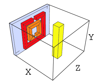
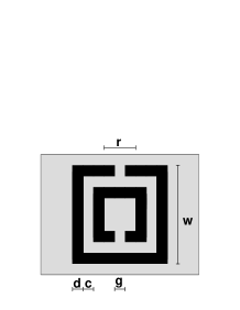
FIG. 1.: Top: The structure of the unit cell as was used in the present simulations. Structure acts as the left-handed meta-material if the electro-magnetic wave propagates along the $z$ direction and is polarized with electric field E parallel to the wire and magnetic field H parallel to the axis of SRR. Bottom: The structure of the SRR and definition of the SRR parameters.

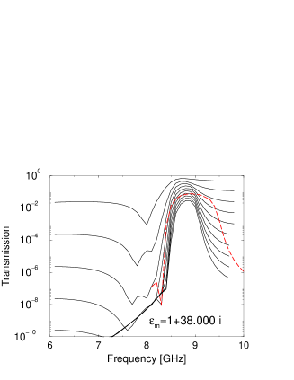
FIG. 2.: LHM peak for various values of the metallic permittivity. Lines corresponds to system length of 1,2,…10 unit cells. SRR is modeled as in Figure 1. The size of the unit cell is $5\times 3.66\times 5$ mm, the size of SRR is 3 mm, and the size of the wire is $1\times 1$ mm. The dashed line is transmission for LHM system with unit cell $3.66\times 3.66\times 3.66$ and the system length of 10 unit cells.

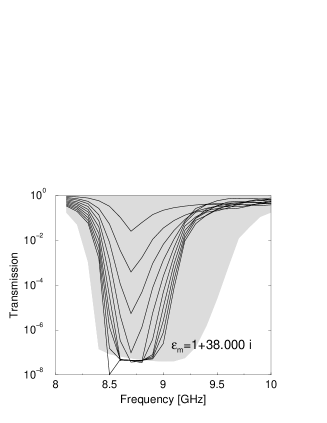
FIG. 3.: Transmission for SRR for the same systems as in Figure 2. Data confirm that the resonance frequency does not depend on the metallic permittivity. This agrees with [19]. However, resonance gap becomes narrower as Im $\epsilon_{\rm m}$ of the metallic components increases. Shaded area represents a gap for the array of the SRR with a unit cell $3.66\times 3.66\times 3.66$ and length system of 10 unit cells. Note also that the depth of the transmission is constant ($\sim 10^{-7}$) and see text for explanation.

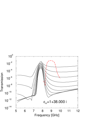
FIG. 4.: Transmission for LHM with the SRR rotated by 90 degrees. The size of the unit cell is now $3.66\times 3.66\times 3.66$ mm. We found no transmission peak for the unit cell size as in Figure 2 (see Figure 11). For comparison with LHM with “up” oriented SRR, we show also the peak for this structure of the same unit cell and metallic permittivity $\epsilon=1+38.000~{}i$ and length system of 10 unit cells (dashed line).

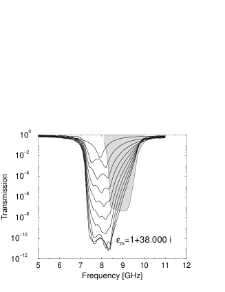
FIG. 5.: Transmission for SRR rotated in 90 degrees. The size of the unit cell is now $3.66\times 3.66\times 3.66$ mm. For comparison, we add also data for the array of “up” SRRs and $\epsilon_{\rm m}=1+38.000~{}i$ and length system of 10 unit cells (shaded area).

FIG. 6.: The transmission for LHM for the same parameters as in Figure 4, but with larger unit cell $5\times 3.66\times 5$ mm. No transmission peak is observed.

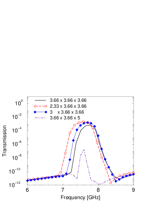
FIG. 7.: Transmission peak for various sizes of the unit cell with “turned” SRR. The system length is 10 unit cells. Resonance frequency decreases slowly as the distance of SRR in the $x$-direction decreases. Increase of the distance of SRR along the $z$ direction causes decrease of the transmission peak, which becomes also much narrower.

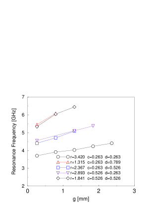
FIG. 8.: Resonance frequency as a function of the azimuthal gap $g$ for various SRR structure. The size of the SRR is 5 mm, the unit cell is $2.63\times 6.05\times 6.05$ mm, which corresponds to $10\times 23\times 23$ mesh points. The ratio $d~{}:~{}c~{}:~{}r$ is 1 : 1 : 13, 3 : 1 : 5, 2 : 1 : 9, 1 : 2 : 11 and 2 : 2 : 7, respectively. Note that azimuthal gap does not enter in Eqn. (4).

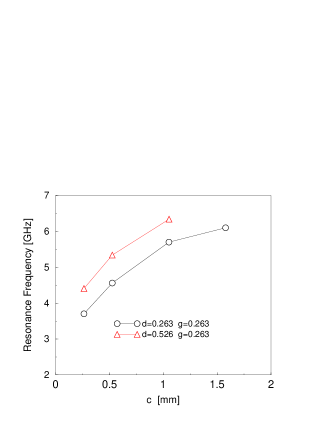
FIG. 9.: Resonance frequency as a function of the radial gap $c$ (distance between rings) for various SRR structures. The size of the sample and of the unit cell is an in Figure 8. In contrast to Eqn. (4), which predicts decrease of $\nu_{0}$ when $c$ increases, we found increase of the resonance frequency. This could be explained by the fact that an increase of the radial gap causes decrease of the inner diameter because $r+2c=3.947$ mm ($\circ$) and 2.895 mm ($\triangle$). Presented data can be therefore interpreted also as the inner diameter - dependence of the resonance frequency. The last ($\nu_{0}\sim r^{-3/2}$) is much stronger than the logarithmic dependence $\nu_{0}\sim\ln^{-1/2}c$. Then, presented data confirm that the decrease of the inner diameter causes an increase of the resonance frequency.

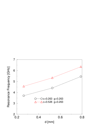
FIG. 10.: Resonance frequency as a function of ring thickness for two sets of SRR. The size of the sample and of the unit cell is an in Figure 8.

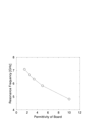
FIG. 11.: Resonance frequency as a function of the permittivity of board. The size of the sample and of the unit cell is an in Figure 8.

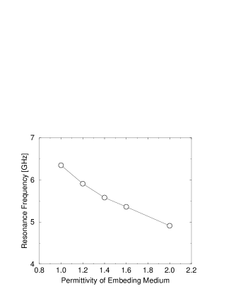
FIG. 12.: Resonance frequency as a function of the permittivity of embedding media in the unit cell (the permittivity of semi-infinite leads remains 1). The size of the sample and of the unit cell is an in Figure 8.

REFERENCES

- [1]
- [2] [*] Permanent address: Institute of Physics, Slovak Academy of Sciences, Dúbravska cesta 9, 842 28 Bratislava, Slovakia. E-mail address: markos@savba.sk
- [3] D. R. Smith, W. J. Padilla, D. C. Vier, S. C. Nemat-Nasser and S. Schultz, Phys. Rev. Lett. 84, 4184 (2000)
- [4] R. A. Shelby, D. R. Smith, S. C. Nemat-Nasser and S. Schultz, Appl. Phys. Lett. 78, 489 (2001)
- [5] J. B. Pendry, A. J. Holden, W. J. Stewart and I. Youngs, Phys. Rev. Lett. 76, 4773 (1996); J. B. Pendry, A. J. Holden, D. J. Robbins and W. J. Stewart, J. Phys.: Cond. Matter 10, 4785 (1998).
- [6] J.B. Pendry, A.J. Holden, D.J. Robbins and W.J. Stewart, IEEE Trans. on Microwave Theory and Techn. 47 2075 (1999)
- [7] J. B. Pendry, Phys. World 13, 27 (2000); Physics Today, May 2000 , p. 17
- [8] V. G. Veselago, Sov. Phys. Usp. 10, 509 (1968).
- [9] D. R. Smith, S. Schultz, N. Kroll, M. Sigalas, K. M. Ho and C. M. Soukoulis, Appl. Phys. Lett. 65, 645 (1994).
- [10] R. A. Shelby, D. R. Smith and S. Schultz, Science 292, 77 (2001).
- [11] D. R. Smith and N. Kroll, Phys. Rev. Lett. 85, 2933 (2000).
- [12] D.R. Smith, S. Schultz, P. Markoš and C.M. Soukoulis, unpublished.
- [13] J. B. Pendry, Phys. Rev. Lett. 85, 3966 (2000).
- [14] J. B. Pendry and A. MacKinnon, Phys. Rev. Lett. 69, 2772 (1992);
- [15] J. B. Pendry, J. Mod. Opt. 41, 209 (1994); J. B. Pendry and P. M. Bell, in Photonic Band Gap Materials, NATO ASI Ser. E 315 (1996) (edited by C.M. Soukoulis) p. 203
- [16] A.J. Ward and J.B. Pendry, J. Mod. Opt. 43, 773 (1996)
- [17] C.M. Soukoulis (editor), Photonic Band Gap Materials, NATO ASI Ser. E 315 (1996)
- [18] J. B. Pendry, A. MacKinnon and P.J. Roberts, Proc. Roy. Soc. London A 437.67, (1992)
- [19] P. Markoš and C.M. Soukoulis, Phys. Rev. B64, to appear in December, 15, 2001 (cond-mat/0105618)
- [20] We analyzed also LHM structures in with Real large and negative simultaneously with Im large and positive (data not presented here). We found that the value of Re influences neither the position of the resonance gap nor the absorption provided that Im is large enough.
- [21] J.D. Jackson: Classical Electrodynamic, J.Willey and Sons, 1962
- [22] In our systems, the symmetry with respect to transformation is broken by presence of the dielectric board with permittivity . This is a reason for non-zero (although very small) values of the transmission and in the “turned” SRR array.
- [23] T. Weiland, R. Schummann, R.B. Gregor, C.G. Parazzoli, A.M. Vetter, R.D. Smith, D.C. Vier and S. Schultz, J. Appl. Phys. (to appear)
- [24] D. Vier, private communication