Investigation of transition frequencies of two acoustically coupled bubbles using a direct numerical simulation technique

Abstract

The theoretical results regarding the “transition frequencies” of two acoustically interacting bubbles have been verified numerically. The theory provided by Ida [Phys. Lett. A 297 (2002) 210] predicted the existence of three transition frequencies per bubble, each of which has the phase difference of $\pi/2$ between a bubble’s pulsation and the external sound field, while previous theories predicted only two natural frequencies which cause such phase shifts. Namely, two of the three transition frequencies correspond to the natural frequencies, while the remaining does not. In a subsequent paper [M. Ida, Phys. Rev. E 67 (2003) 056617], it was shown theoretically that transition frequencies other than the natural frequencies may cause the sign reversal of the secondary Bjerknes force acting between pulsating bubbles. In the present study, we employ a direct numerical simulation technique that uses the compressible Navier–Stokes equations with a surface-tension term as the governing equations to investigate the transition frequencies of two coupled bubbles by observing their pulsation amplitudes and directions of translational motion, both of which change as the driving frequency changes. The numerical results reproduce the recent theoretical predictions, validating the existence of the transition frequencies not corresponding to the natural frequency.

1 Introduction

The secondary Bjerknes force is an interaction force acting between pulsating gas bubbles in an acoustic field.[1, 2, 3] The classical theory originated by Bjerknes predicts either attraction only or repulsion only, depending on whether the driving frequency stays outside or inside, respectively, the frequency region between the partial (or monopole) natural frequencies of two bubbles. However, recent studies show that the force sometimes reverses its own direction as the distance between the bubbles changes.[4, 5, 6] The first theoretical study on this subject was performed by Zabolotskaya.[4] Employing a linear coupled oscillator model, she showed that the radiative interaction between the bubbles, which results in the change in the natural frequencies of the bubbles, could cause this reversal. In the mid-1990s, Doinikov and Zavtrak arrived at the same conclusion by employing a linear theoretical model in which the multiple scattering between the bubbles is more rigorously taken into account.[5] These theoretical results are considered to explain the stable structure formation of bubbles in a sound field, called “bubble cluster” or “bubble grape,” which has been observed experimentally by several researchers in different fields.[7, 8, 9, 10, 11, 3]

In both of the theoretical studies mentioned above, it was assumed that the reversal is due to the change in the natural (or the resonance) frequencies of bubbles, caused by the radiative interaction between bubbles. However, those authors had differing interpretations of how the natural frequencies change. The theoretical formula for the natural frequencies, used by Zabolotskaya[4] and given previously by Shima,[12] shows that the higher and the lower natural frequencies (converging to the partial natural frequencies of a smaller and a larger bubble, respectively, when the distance between the bubbles is infinite) reveal an upward and a downward shift, respectively, as the bubbles come closer to one another.[12, 13] In contrast, Doinikov and Zavtrak assumed intuitively that both the natural frequencies rise.[5, 6] This assumption seems to explain well the sign reversal occurring not only when both bubbles are larger than the resonance size but also when one bubble is larger and the other is smaller than the resonance size. The sign reversal in the latter case, for instance, is thought to occur when the resonance frequency of a larger bubble, increasing as the bubbles come closer to one another, surpasses the driving frequency, resulting in the change in the pulsation phase of the larger bubble, and leading to the change in the phase difference between the bubbles. However, this assumption is obviously inconsistent with the previous theoretical result for the natural frequencies.[12, 4]

Recently, Ida[14] proposed an alternative theoretical explanation for this phenomenon, also using the linear model Zabolotskaya used. He claimed that this phenomenon cannot be interpreted by only observing the natural frequencies, and that it is useful to define the transition frequencies that make the phase difference between a bubble’s pulsation and an external sound $\pi/2$ (or $3\pi/2)$. It has been pointed out theoretically that the maximum number of natural frequencies and that of transition frequencies are, in general, not in agreement in multibubble cases,[13, 15] while they are, as is well known, consistent in single-bubble cases where the phase difference between a bubble’s pulsation and an external sound becomes $\pi/2$ only at its natural frequency. (This is not true in strongly nonlinear cases, in which the phase reversal can take place even in frequency regions far from the bubble’s natural frequency; see, e.g., refs. ref16,ref17.) In a double-bubble case, for instance, that theory predicts three transition frequencies per bubble, two of which correspond to the natural frequencies.[13] A preliminary discussion on a $N$-bubble system[15] showed that a bubble in this system has up to $2N-1$ transition frequencies, only $N$ ones of which correspond to the natural frequencies. More specifically, the number of transition frequencies is in general larger than that of natural frequencies. The transition frequencies not corresponding to the natural frequency have differing physical meanings from those of the natural frequencies; they do not cause the resonance response of the bubbles.[13, 15] The theory for the sign reversal of the force, constructed based on the transition frequencies, predicts that the sign reversal takes place around those frequencies, not around the natural frequencies, and can explain the sign reversal in both cases mentioned above.[14] Moreover, the theory does not contradict the theory for the natural frequencies described previously, because all the natural frequencies are included in the transition frequencies.

The aim of this paper is to verify the theoretical prediction of the transition frequencies by direct numerical simulation (DNS). In a recent paper,[18] Ida proposed a DNS technique, based on a hybrid advection scheme,[19] a multi-time-step integration technique,[18] and the Cubic-Interpolated Propagation/Combined, Unified Procedure (CIP–CUP) algorithm,[20, 21] which technique allows us to compute the dynamics (pulsation and translational motion) of deformable bubbles in a viscous liquid even when the separation distance between the bubbles is small.[18, 22] In that DNS technique, the compressible Navier–Stokes equations with a surface-tension term are selected as the governing equations, and the convection, the acoustic, and the surface-tension terms, respectively, in these equations are solved by an explicit advection scheme employing both interpolation and extrapolation functions which realizes a discontinuous description of interfaces between different materials,[19] by the Combined, Unified Procedure (CUP) being an implicit finite difference method for all-Mach-number flows,[20, 21] and by the Continuum Surface Force (CSF) model being a finite difference solver for the surface-tension term as a volume force.[23] Efficient and accurate time integration of the compressible Navier–Stokes equations under a low-Mach-number condition is achieved by the multi-time-step integration technique,[18] which solves the different-nature terms in these equations with different time steps. Further details of this DNS technique can be found in refs. ref18,ref19. Employing this DNS technique, in the present study we perform numerical experiments involving two acoustically coupled bubbles in order to investigate the recent theories by observing the bubbles’ pulsation amplitudes and the directions of their translational motion. In particular, we focus our attention on the existence of the transition frequencies that do not cause the resonance response.

The following sections are organized as follows. In §2, the previously expounded theories are reviewed and reexamined, including those for the transition frequencies and the sign reversal, and in §3, the numerical results and a discussion are provided. Section 4 presents concluding remarks.

2 Theories

2.1 A single-bubble problem

It is well known that, when the wavelength of an external sound is sufficiently large compared to the radius of a bubble (named “bubble 1,” immersed in a liquid) and the sphericity of the bubble is maintained, the following second-order differential equation[3, 24] describes the linear pulsation of the bubble:

$$\ddot{e}_{1}+\omega_{10}^{2}e_{1}+\delta_{1}\dot{e}_{1}=-\frac{p_{\rm{ex}}}{\rho_{0}R_{10}},$$ (1)

$$\omega_{10}=\sqrt{\frac{1}{\rho_{0}R_{10}^{2}}\left[{3\kappa P_{0}+(3\kappa-1)\frac{2\sigma}{R_{10}}}\right]},$$

where it is assumed that the bubble’s time-dependent radius can be represented by $R_{1}=R_{10}+e_{1}$ ($\left|{e_{1}}\right|\ll R_{10})$ with $R_{10}$ being its equilibrium radius and $e_{1}$ being the deviation in the radius, and $\omega_{10}$ is the bubble’s natural frequency, $\delta_{1}$ is the damping factor,[25, 26] $p_{\rm{ex}}$ is the sound pressure at the bubble position, $\rho_{0}$ is the equilibrium density of the liquid, $P_{0}$ is the static pressure, $\kappa$ is the polytropic exponent of the gas inside the bubble, $\sigma$ is the surface tension, and the over dots denote the derivation with respect to time. Assuming $p_{\rm{ex}}=-P_{a}\sin\omega t$ (where $P_{a}$ is a positive constant), the harmonic steady-state solution of eq. (1) is determined as

$$e_{1}=K_{S1}\sin(\omega t-\phi_{S1}),$$

where

$$K_{S1}=\frac{P_{a}}{\rho_{0}R_{10}}\sqrt{\frac{1}{(\omega_{10}^{2}-\omega^{2})^{2}+\delta_{1}^{2}\omega^{2}}},$$

$$\phi_{S1}=\tan^{-1}\left({\frac{\delta_{1}\omega}{\omega_{10}^{2}-\omega^{2}}}\right).$$

This result reveals that the phase reversal (or the phase difference of $\phi_{S1}=\pi/2)$ appears at only $\omega=\omega_{10}$. Moreover, if $\delta_{1}\ll\omega_{10}$, the bubble’s resonance response can take place at almost the same frequency. Though the resonance frequency shifts away from $\omega_{10}$ as $\delta_{1}$ increases, it can in many cases be assumed to be almost the same as $\omega_{10}$. (Also, the nonlinearity in bubble pulsation is known to alter a bubble’s resonance frequency.[2, 3, 27])

2.2 A double-bubble problem

When one other bubble (bubble 2) exists, the pulsation of the previous bubble is driven by not only the external sound but also the sound wave that bubble 2 radiates. Assuming that the surrounding liquid is incompressible and the time-dependent radius of bubble 2 can be represented by $R_{2}=R_{20}+e_{2}$ ($\left|{e_{2}}\right|\ll R_{20})$, the radiated pressure field is found to be,[15]

$$p(r,t)\approx\frac{\rho_{0}R_{20}^{2}}{r}\ddot{e}_{2},$$

where $r$ is the distance measured from the center of bubble 2. The total sound pressure at the position of bubble 1 ($p_{\rm{d1}})$ is, thus,

$$p_{\rm{d1}}\approx p_{\rm{ex}}+\frac{\rho_{0}R_{20}^{2}}{D}\ddot{e}_{2},$$ (2)

where $D$ is the distance between the centers of the bubbles. This total pressure drives the pulsation of bubble 1.

Replacing $p_{\rm{ex}}$ in eq. (1) with $p_{\rm{d1}}$ yields the modified equation for bubble 1,

$$\ddot{e}_{1}+\omega_{10}^{2}e_{1}+\delta_{1}\dot{e}_{1}=-\frac{p_{\rm{ex}}}{\rho_{0}R_{10}}-\frac{R_{20}^{2}}{R_{10}D}\ddot{e}_{2},$$ (3)

and exchanging 1 and 2 (or 10 and 20) in the subscripts in this equation yields that for bubble 2,

$$\ddot{e}_{2}+\omega_{20}^{2}e_{2}+\delta_{2}\dot{e}_{2}=-\frac{p_{\rm{ex}}}{\rho_{0}R_{20}}-\frac{R_{10}^{2}}{R_{20}D}\ddot{e}_{1}.$$ (4)

This kind of system of differential equations is called a (linear) coupled oscillator model or a self-consistent model,[28, 29] and is known to be third-order accuracy with respect to $1/D$.[30] The same (or essentially the same) formula has been employed in several studies considering acoustic properties of coupled bubbles.[4, 12, 28, 29, 30, 31, 32]

Shima[12] and Zabolotskaya,[4] assuming $\delta_{j}\approx 0$ (for $j=1$ and 2), derived the theoretical formula for the natural frequencies, represented as

$$(\omega_{10}^{2}-\omega^{2})(\omega_{20}^{2}-\omega^{2})-\frac{R_{10}R_{20}}{D^{2}}\omega^{4}=0.$$ (5)

This equation predicts the existence of up to two natural frequencies (or eigenvalues of the system (3) and (4)) per bubble. Exchanging 10 and 20 in the subscripts in this equation yields the same equation; namely, when $\delta_{j}\approx 0$, both the bubbles have the same natural frequencies. The higher and the lower natural frequencies reveal an upward and a downward shift, respectively, as $D$ decreases.[12, 13]

The theoretical formula for the transition frequencies, derived by Ida,[13] can be obtained based on the harmonic steady-state solution of system (3) and (4). Assuming $p_{\rm{ex}}=-P_{a}\sin\omega t$, the solution is determined as follows:

$$e_{1}=K_{1}\sin(\omega t-\phi_{1}),$$ (6)

where

$$K_{1}=\frac{P_{a}}{R_{10}\rho_{0}}\sqrt{A_{1}^{2}+B_{1}^{2}},$$ (7)

$$\phi_{1}=\tan^{-1}\left({\frac{B_{1}}{A_{1}}}\right)$$ (8)

with

$$A_{1}=\frac{H_{1}F+M_{2}G}{F^{2}+G^{2}},\quad B_{1}=\frac{H_{1}G-M_{2}F}{F^{2}+G^{2}},$$

$$F=L_{1}L_{2}-\frac{R_{10}R_{20}}{D^{2}}\omega^{4}-M_{1}M_{2},$$

$$G=L_{1}M_{2}+L_{2}M_{1},\quad H_{1}=L_{2}+\frac{R_{20}}{D}\omega^{2},$$

$$L_{1}=\omega_{10}^{2}-\omega^{2},\quad L_{2}=\omega_{20}^{2}-\omega^{2},$$

$$M_{1}=\delta_{1}\omega,\quad M_{2}=\delta_{2}\omega.$$

Exchanging 1 and 2 (or 10 and 20) in the subscripts in these equations yields the formula for bubble 2. Based on the definition, the transition frequencies are given by[13]

$$H_{1}F+M_{2}G=0.$$ (9)

This equation predicts the existence of up to three transition frequencies per bubble[13]; this number is greater than that of the natural frequencies given by eq. (5). This result means that in a multibubble case, the phase shift can take place not only around the bubbles’ natural frequencies but also around some other frequencies. Moreover, it was shown in ref. ref13 that the transition frequencies other than the natural frequencies do not cause the resonance response; namely, one of the three transition frequencies has different physical meanings from those of the natural frequency.

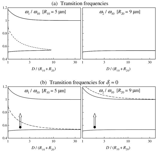
Figure 1: Transition frequencies as functions of the distance between the bubbles. The lower figure shows the transition frequencies in the case where the damping effect is neglected. The dashed lines denote the transition frequencies that do not cause resonance. The arrows are used for a discussion described in the text.

Figure 1(a) shows the transition frequencies of bubbles 1 and 2, $\omega_{1}$ and $\omega_{2}$, for $R_{10}=5$ $\mu$m and $R_{20}=9$ $\mu$m, as functions of $D/(R_{10}+R_{20})$. These bubble radii are chosen to be small enough so that the sphericity of the bubbles is maintained sufficiently. The parameters are set to $\rho_{0}=1000$ kg/m³, $\kappa=1.33$, $P_{0}=1$ atm, and $\sigma=0.0728$ N/m. The damping factors are determined by the sum of the viscous and radiation ones as $\delta_{j}=(4\mu/\rho_{0}R_{j0}^{2})+(\omega^{2}R_{j0}/c)$ since the DNS technique does not consider the thermal conduction,[18] where the viscosity of the liquid $\mu=1.137\times 10^{-3}$ kg/(m s) and its sound speed $c=1500$ m/s. As a reference, in Fig. 1(b) we display the transition frequencies for $\delta_{j}\to 0$. As discussed previously,[13] the highest and the second highest transition frequencies of the larger bubble tend to vanish when the damping effect is sufficiently strong; in the present case, they disappear completely. The second highest and the lowest transition frequencies of the smaller bubble cross and vanish at a certain distance, and only one transition frequency remains for sufficiently large $D$. For $D\to\infty$, the transition frequencies remaining converge to the partial natural frequencies of the corresponding bubble. The solid lines displayed in Fig. 1(b) denote the transition frequencies that correspond to the natural frequencies given by eq. (5).

We clarify here physical meanings of the transition frequencies that do not accompany resonance, which meanings have not yet been described in the literature. Let us consider the bubbles under the condition indicated by the dots (the origin of the arrows) shown in Fig. 1. Bubble 2 under this condition emits a strong sound (denoted below by $p_{2}(D)$) whose oscillation phase is (almost) out-of-phase with the external sound $p_{{\rm ex}}$, because the driving frequency stays near and slightly above the natural frequency of this bubble. If $p_{2}(D)$ is measured at a point sufficiently near bubble 2, its amplitude can be larger than that of $p_{{\rm ex}}$ and hence the phase of the total sound pressure, $p_{{\rm ex}}+p_{2}(D)$, may be almost the same as that of $p_{2}(D)$, i.e., almost out-of-phase with $p_{{\rm ex}}$. As the driving frequency shifts toward a higher range along the arrows, the absolute value of $p_{2}(D)$ decreases and, at a certain frequency, becomes lower than $\left|{p_{{\rm ex}}}\right|$; the phase of the total sound pressure finally becomes (almost) in-phase with $p_{{\rm ex}}$. This transition of the power balance of the two sounds results in the phase reversal of bubble 1 without accompanying the resonance response.

2.3 The secondary Bjerknes force

The secondary Bjerknes force acting between two pulsating bubbles is represented by[1, 2, 3]

$${\rm{\bf F}}\propto\langle{\dot{V}_{1}\dot{V}_{2}}\rangle\frac{{\rm{\bf r}}_{2}-{\rm{\bf r}}_{1}}{\left\|{{\rm{\bf r}}_{2}-{\rm{\bf r}}_{1}}\right\|^{3}},$$ (10)

where $V_{j}$ and ${\rm{\bf r}}_{j}$ denote the volume and the position vector, respectively, of bubble $j$, and $\langle\cdots\rangle$ denotes the time average. Using eqs. (6)–(8), this equation can be rewritten as[1]

$${\rm{\bf F}}\propto K_{1}K_{2}\cos(\phi_{1}-\phi_{2})\frac{{\rm{\bf r}}_{2}-{\rm{\bf r}}_{1}}{\left\|{{\rm{\bf r}}_{2}-{\rm{\bf r}}_{1}}\right\|^{3}}.$$ (11)

The sign reversal of this force occurs only when the sign of $\cos(\phi_{1}-\phi_{2})$ (or of $\langle{\dot{V}_{1}\dot{V}_{2}}\rangle)$ changes, because $K_{1}>0$ and $K_{2}>0$. Namely, the phase property of the bubbles plays an important role in the determination of the sign. Roughly speaking, the force is attractive when the bubbles pulsate in-phase with each other, while it is repulsive when they pulsate out-of-phase.

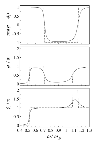
Figure 2: Sign of the secondary Bjerknes force [$\cos(\phi_{1}-\phi_{2})$] and phase differences [$\phi_{1}$ and $\phi_{2}$], determined theoretically, as functions of the driving angular frequency. The positive value of $\cos(\phi_{1}-\phi_{2})$ indicates the attraction, while the negative one indicates the repulsion. The dashed lines denote the results for $\delta_{j}\approx 0$.

The solid lines displayed in Fig. 2 denote $\cos(\phi_{1}-\phi_{2})$, $\phi_{1}$, and $\phi_{2}$ as functions of $\omega/\omega_{10}$, and the dashed lines denote those for $\delta_{j}\approx 0$. The physical parameters are the same as used for Fig. 1, except for the separation distance fixed to $D=20$ $\mu$m [$D/(R_{10}+R_{20})\approx 1.43]$. In this figure, we can observe sign reversals of $\cos(\phi_{1}-\phi_{2})$ at $\omega/\omega_{10}\approx 0.72$ and $\omega/\omega_{10}\approx 1.15$. In ref. ref14, it was shown theoretically that both the sign reversals are due to the transition frequencies that do not correspond to the natural frequencies; that is, the sign reversals take place near (or, when $\delta_{j}\to 0$, at) those frequencies. The present result follows that theoretical prediction. The respective reversals are observed near the second highest transition frequency of bubble 1 and near the highest of bubble 2 for $\delta_{j}\to 0$. Meanwhile, we can observe $\phi_{2}>\pi$, which should not be observed in a single-bubble case. Ida[14] explained that such a large phase delay is realizable in a multibubble case, by the radiative interaction.

We make here a remark regarding the estimation of the points at which the sign reversal of the force takes place. It was shown previously[14] that the transition points of the force are hardly changed by the damping effects, even when bubbles are small ($R_{j0}\sim 1$ $\mu$m) or relatively large ($R_{j0}\sim 1$ mm). The present result displayed in Fig. 2 follows that finding. These results may allow us to consider that the simple theoretical formulas for the transition frequencies not causing resonance,

$$\omega_{1}^{2}=\frac{\omega_{20}^{2}}{1-R_{20}/D}\quad\mbox{and}\quad\omega_{2}^{2}=\frac{\omega_{10}^{2}}{1-R_{10}/D}$$

derived for $\delta_{1}\to 0$ and $\delta_{2}\to 0$,[13] can be a good approximation of the transition points, even in the cases of $\delta_{j}\neq 0$. These formulas yield $(\omega_{1}/\omega_{10})=0.719$ and $(\omega_{2}/\omega_{10})=1.155$, which are consistent with the result shown in Fig. 2.

3 Numerical results and discussion

In this section, the DNS technique[18, 19] is employed to verify the theoretical results for the transition frequencies. The governing equations are the compressible Navier–Stokes equations

$$\frac{\partial\rho}{\partial\,t}+{\rm{\bf u}}\cdot\nabla\rho=-\rho\nabla\cdot{\rm{\bf u}},$$

$$\frac{\partial{\rm{\bf u}}}{\partial t}+{\rm{\bf u}}\cdot\nabla{\rm{\bf u}}=-\frac{\nabla p}{\rho}+\frac{1}{\rho}\left({2\nabla\cdot(\mu{\rm{\bf T}})-\frac{2}{3}\nabla(\mu\nabla\cdot{\rm{\bf u}})}\right)+\frac{{\rm{\bf F}}_{st}}{\rho},$$

$$\frac{\partial p}{\partial\,t}+{\rm{\bf u}}\cdot\nabla p=-\rho C_{S}^{2}\nabla\cdot{\rm{\bf u}},$$

where $\rho$, ${\rm{\bf u}}$, $p$, ${\rm{\bf T}}$, $\mu$, ${\rm{\bf F}}_{st}$, and $C_{S}$ denote the density, the velocity vector, the pressure, the deformation tensor, the viscosity coefficient, the surface tension as a volume force, and the local sound speed, respectively. This system of equations is solved over the whole computational domain divided by grids. The materials (the bubbles and a liquid surrounding them) moving on the computational grids are identified by a scalar function[19] depending on a pure advection equation whose characteristic velocity is ${\rm{\bf u}}$. The bubbles’ radii and the initial center-to-center distance between them are set by using the same values as used for Fig. 2, that is, $R_{10}=5$ $\mu$m, $R_{20}=9$ $\mu$m, and $D(t=0)=20$ $\mu$m. The content inside the bubbles is assumed to be an ideal gas with a specific heat ratio of 1.33, an equilibrium density of 1.23 kg/m³, and a viscosity of $1.78\times 10^{-5}$ kg/(m s). The surrounding liquid is water, whose sound speed is determined by $C_{S}=\sqrt{7(p+3172.04P_{0})/\rho}$ with $p$ and $\rho$ being the local pressure and density, respectively. The other parameters are set to the same values as those used previously. The axisymmetric coordinate ($r,z)$ is selected for the computational domain, and the mass centers of the bubbles are located on the central axis of the coordinate. The grid widths are set to be constants as $\Delta r=\Delta z=0.25$ $\mu$m, and the numbers of them in the $r$ and the $z$ coordinates are 100 and 320, respectively. The sound pressure, applied as the boundary condition to the pressure, is assumed to be in the form of $p_{\rm{ex}}=P_{a}\sin\omega t$, where the amplitude $P_{a}$ is fixed to $0.3P_{0}$ and the driving frequency is selected from the frequency range around the bubbles’ partial natural frequencies. (For the sound amplitude assumed, nonlinear effects may not completely be neglected especially near the natural frequencies. However, we can, unfortunately, not use a lower sound pressure because of a numerical problem called “parasitic currents,”[33, 34] which rise to the surface when a small bubble or drop is in (nearly) steady state where the amplitudes of volume and shape oscillations are very low. Effects of nonlinearity are briefly discussed later.) The boundary condition for the velocity is free.

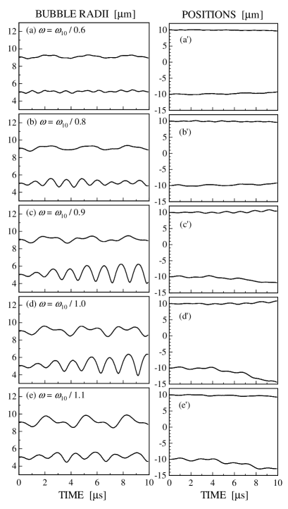
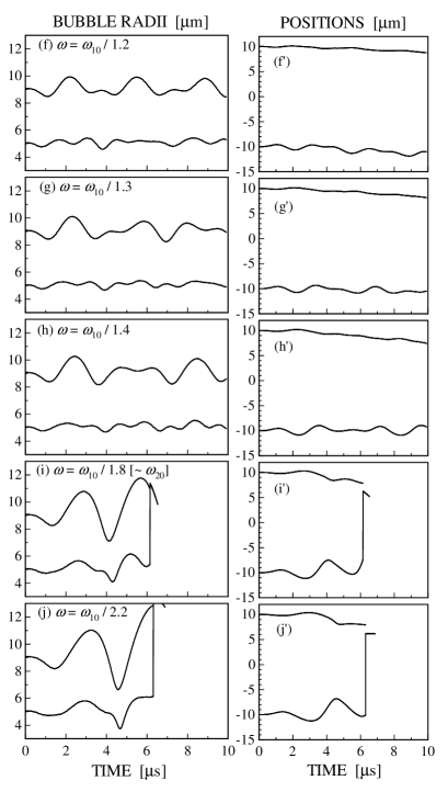
Figure 3: DNS results: Bubble radii [(a) $\sim$ (j)] and corresponding positions [(a’) $\sim$ (j’)] as functions of time for different driving frequencies. The lower lines in (a’)–(j’) denote the position of the smaller bubble. The bubbles coalesce at the time where the number of lines becomes one, see panels (i), (i’), (j), and (j’).

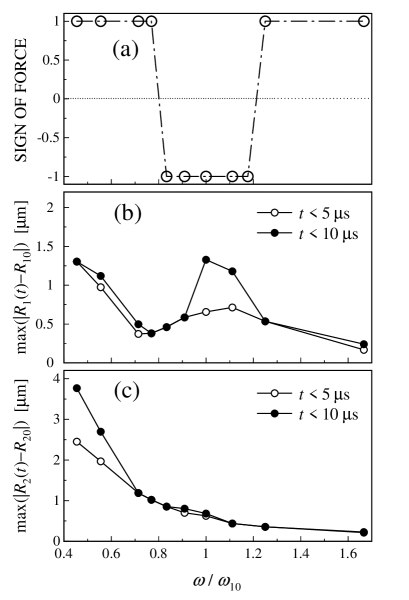
Figure 4: DNS results: (a) Sign of the force, (b) pulsation amplitude of bubble 1, and (c) that of bubble 2, as functions of the driving frequency. The amplitudes were measured for $t<5$ $\mu$s ($\circ$), and for $t<10$ $\mu$s but until the coalescence has been observed ($\bullet$). The result for $\omega=\omega_{10}/0.85$, not shown in Fig. 3, is presented in (a); see also Fig. 5.

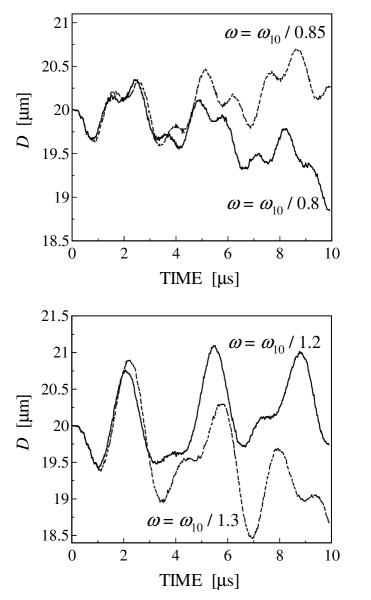
Figure 5: Time-dependent distances between the mass centers of the bubbles in the cases where the deviation in the distance is small (for $\omega=\omega_{10}/0.8$, $\omega_{10}/0.85$, $\omega_{10}/1.2$, and $\omega_{10}/1.3$). Note that the result for $\omega=\omega_{10}/0.85$, not shown in Fig. 3, is added. [The low-amplitude, high-frequency oscillations observed in these curves may be due to a numerical error originating in the calculation of such a small deviation (comparable to the grid width) on a discrete computational domain.]

Figure 3 displays the bubbles’ (mean) radii and mass centers as functions of time for different $\omega$, and figure 4 displays the sign of the force (a), determined by observing the direction of the bubbles’ translation, and the bubbles’ pulsation amplitudes (b and c). From these figures, we know that the smaller bubble has two resonance frequencies, one at $\omega\approx\omega_{10}/0.9$ ($\approx 1.1\omega_{10})$ and the other at $\omega\approx\omega_{10}/2.2$ ($\approx 0.45\omega_{10})$, though the former seems to decrease with time because of the repulsion of the bubbles (See Fig. 1, which reveals that the highest transition frequency of bubble 1, causing resonance, decreases as $D$ increases). The former resonance frequency is higher than $\omega_{10}$, and the latter is lower than $\omega_{20}$ ($\approx 0.53\omega_{10})$. These respective resonances are obviously due to the highest and the lowest transition frequencies of bubble 1, both of which correspond to the natural frequencies. The same figure shows that the larger bubble may have a resonance frequency, at $\omega\approx\omega_{10}/2.2$.

The sign of the interaction force changed twice in the frequency region considered. In the region between $\omega=\omega_{10}/0.8$ and $\omega_{10}/0.9$, being near to but above the higher resonance frequency of the smaller bubble discussed above, the attractive force turns into repulsion as $\omega$ decreases, and, at $\omega\approx\omega_{10}/1.2$ ($\approx 0.83\omega_{10})$ the repulsive force turns back into attraction. (See also Fig. 5, which shows $D(t)$ in the cases where the deviation in it is small.) It may be difficult to say, using only these numerical results, that the former reversal is not due to the higher natural frequency of the smaller bubble, because the reversal took place near it and the highest transition frequency of the larger bubble is close to it. Therefore, in the following we will focus our attention on the latter sign reversal, which occurred at $\omega$ between $\omega_{10}$ and $\omega_{20}$.

The latter reversal indicates that a kind of characteristic frequency should exist in the frequency region between the partial natural frequencies of the bubbles. It is evident that this characteristic frequency is not the resonance frequency of the larger bubble, which is, as already discussed, much lower. This result is in opposition to the assumption described by Doinikov and Zavtrak.[5, 6] Also, the theory for the natural frequencies (eq. (5)) cannot explain this reversal, because it predicts no natural frequency in the frequency region between $\omega_{10}$ and $\omega_{20}$. This characteristic frequency is, arguably, the second highest transition frequency of the smaller bubble, as was predicted by Ida.[14] As was proved theoretically in ref. ref13, resonance response is not observed around this characteristic frequency. In order to confirm that this characteristic frequency is not of the larger bubble, we display in Fig. 6 the $R_{2}$–time and $p_{\rm{ex}}$–time curves for the area around $\omega=\omega_{10}/1.2$. This figure shows clearly that the pulsation phase of the larger bubble does not reverse in this frequency region; the bubble maintains its out-of-phase pulsation with the external sound (i.e., the bubble’s radius is large when the sound amplitude is positive), although other modes, which may result from the transient, appear.

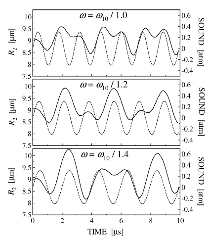
Figure 6: Radius of the larger bubble (solid lines) and sound pressure as functions of time, for around $\omega=\omega_{10}/1.2$.

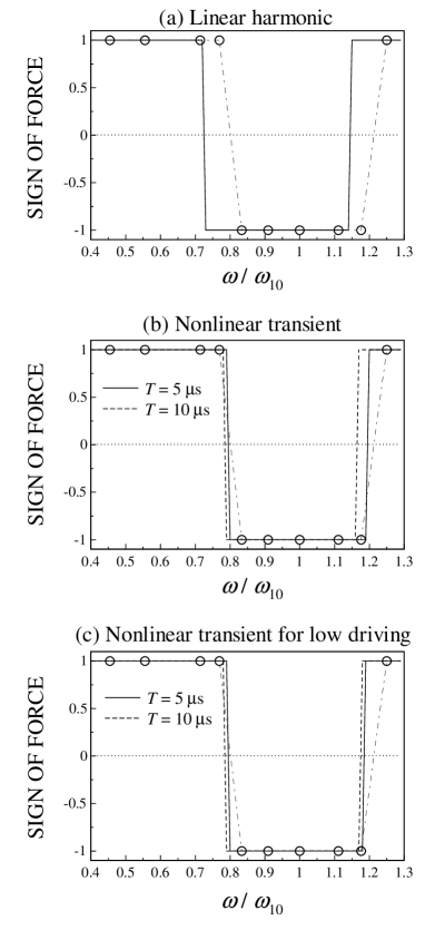
Figure 7: Comparison of the DNS results with (a) the linear harmonic solution, (b) the nonlinear numerical results for $P_{a}=0.3P_{0}$, and (c) those for $P_{a}=0.001P_{0}$. The circles denote the DNS results, where the positive value denotes the attraction while the negative value denotes the repulsion.

Here, we discuss how this transient and a nonlinear effect act on the quantitative nature of the sign distribution. In Fig. 7(a), we show the sign of the force as functions of $\omega$, determined by the linear theory (the solid line) and by the DNS (the circles). The positive value denotes the attraction, while the negative value the repulsion. A noticeable quantitative discrepancy can be observed between these results, whereas they are in agreement in a qualitative sense. We attempt here to identify what caused this discrepancy, using a nonlinear model. Mettin et al. [35] proposed a nonlinear coupled oscillator model for a double-bubble system,

$$\left({1-\frac{\dot{R}_{1}}{c}}\right)R_{1}\ddot{R}_{1}+\left({\frac{3}{2}-\frac{\dot{R}_{1}}{2c}}\right)\dot{R}_{1}^{2}=\frac{1}{\rho_{0}}\left({1+\frac{\dot{R}_{1}}{c}}\right)p_{\rm{k}\,1}+\frac{R_{1}}{\rho_{0}c}\frac{dp_{\rm{k}\;1}}{dt}-\frac{1}{D}\frac{d}{dt}(\dot{R}_{2}R_{2}^{2}),$$ (12)

$$\left({1-\frac{\dot{R}_{2}}{c}}\right)R_{2}\ddot{R}_{2}+\left({\frac{3}{2}-\frac{\dot{R}_{2}}{2c}}\right)\dot{R}_{2}^{2}=\frac{1}{\rho_{0}}\left({1+\frac{\dot{R}_{2}}{c}}\right)p_{\rm{k}\,2}+\frac{R_{2}}{\rho_{0}c}\frac{dp_{\rm{k}\,2}}{dt}-\frac{1}{D}\frac{d}{dt}(\dot{R}_{1}R_{1}^{2}),$$ (13)

with

$$p_{\rm{k}\,j}=\left({P_{0}+\frac{2\sigma}{R_{j0}}}\right)\left({\frac{R_{j0}}{R_{j}}}\right)^{3\kappa}-\frac{2\sigma}{R_{j}}-\frac{4\mu\dot{R}_{j}}{R_{j}}-P_{0}-p_{\rm{ex}}\quad\mbox{for}\;j=1\mbox{ or }2,$$

based on the Keller–Miksis model[36] taking into account the viscosity and compressibility of the surrounding liquid with first-order accuracy. In this system of equations, the last terms of eqs. (12) and (13) represent the radiative interaction between the bubbles. Using this model, $R_{j}$ and $\dot{R}_{j}$ are calculated by the fourth-order Runge–Kutta method, and subsequently the time average in eq. (10) is performed to determine the sign of the force. Although the quantitative accuracy of this model may not be guaranteed for a small $D$,[35] a rough estimation of the influences of the transient and nonlinearity might be achieved. The physical parameters are the same as used for Fig. 1, and $D$ is fixed to $20$ $\mu$m, that is, the translational motion is neglected. The solid and the dashed lines displayed in Fig. 7(b) show

$$G(T)\equiv{\rm sgn}\left[{{\int_{0}^{T}{\dot{V}_{1}\dot{V}_{2}dt}}\mathord{\left/{\vphantom{{\int_{0}^{T}{\dot{V}_{1}\dot{V}_{2}dt}}T}}\right.\kern-1.2pt}T}\right]$$

for $T=5$ $\mu$s and 10 $\mu$s, respectively, given using the nonlinear model, where ${\rm sgn}[f]=1$ for $f>0$ and ${\rm sgn}[f]=-1$ otherwise. These numerical results are in good agreement with the DNS results (the circles). Figure 7(c) shows the numerical results given using the nonlinear model with a very low driving pressure ($P_{a}=0.001P_{0})$. These results are also in good agreement with the DNS results, proving that, in the present case, the nonlinearity in the pulsations is not dominant for the sign reversals. Furthermore, it can be proved that the bubbles’ shape oscillation is also not dominant for the sign reversal. Figure 8 shows the bubble surfaces for $\omega=\omega_{10}/1.2$ at selected times. Only a small deformation of the bubbles can be found in this figure. (The numerical results provided previously in ref. ref18, given using the same DNS technique, reveal that the bubbles’ sphericity is well maintained even for $\omega=\omega_{10}$, whereas a noticeable deformation is observed for $\omega\approx\omega_{20}$.) These results allow us to consider that the transient is one of the dominant origins of the noticeable quantitative discrepancy found in Fig. 7(a).

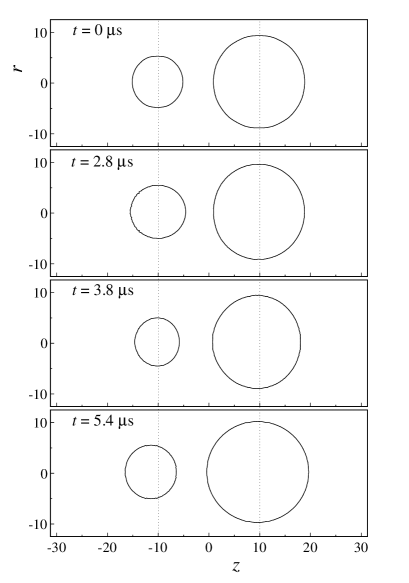
Figure 8: Bubble surfaces for $\omega=\omega_{10}/1.2$ at selected times, given by the DNS technique. Similar figures for $\omega=\omega_{10}$ and $\omega=\omega_{10}/1.8$ can be found in our previous paper [18].

There are some other physical factors that may also be able to cause the quantitative discrepancy but are not taken into account in both the linear and nonlinear coupled oscillator models. It is known, for example, that the translational motion of bubbles can alter the bubbles’ pulsation. As has been proved by several researchers,[37, 38, 30] if the translational motion is taken into consideration in deriving a theoretical model, high-order terms appear in the equations of radial motion, in which not only the bubbles’ radii but also their translational velocities are involved. Also, in certain cases the viscosity of the surrounding liquid can alter the magnitude and sign of the interaction force, because acoustic streaming is induced around the bubbles.[39] Investigating the influences of those factors on the quantitative discrepancy using a higher-order model would be an interesting and important subject.

4 Concluding remarks

In summary, we have verified the recent theoretical results regarding the transition frequencies of two acoustically interacting bubbles[13] and the sign reversal of the secondary Bjerknes force,[14] using a DNS technique.[18, 19] The present numerical results, given by the DNS technique, support those theoretical results at least in a qualitative sense. The most important point validated by DNS is that at least the sign reversal occurring when the driving frequency stays between the bubbles’ partial natural frequencies is obviously not due to the natural (or the resonance) frequencies of the double-bubble system. This conclusion is in opposition to the previous explanation described by Doinikov and Zavtrak,[5, 6] but is consistent with the most recent interpretation by Ida[14] described based on analyses of the transition frequencies,[13, 15] thus validating the assertion that the transition frequencies not corresponding to the natural frequencies exist and that the notion “transition frequency” is useful for understanding the sign reversal of the force.

References

- [1] L. A. Crum: J. Acoust. Soc. Am. 57 (1975) 1363.
- [2] A. Prosperetti: Ultrasonics 22 (1984) 115.
- [3] W. Lauterborn, T. Kurz, R. Mettin and C. D. Ohl: Adv. Chem. Phys. 110 (1999) 295.
- [4] E. A. Zabolotskaya: Sov. Phys. Acoust. 30 (1984) 365.
- [5] A. A. Doinikov and S. T. Zavtrak: Phys. Fluids 7 (1995) 1923.
- [6] A. A. Doinikov and S. T. Zavtrak: J. Acoust. Soc. Am. 99 (1996) 3849.
- [7] Y. A. Kobelev, L. A. Ostrovskii and A. M. Sutin: JETP Lett. 30 (1979) 395.
- [8] P. L. Marston, E. H. Trinh, J. Depew and T. J. Asaki, in: Bubble Dynamics and Interface Phenomena, edited by J. R. Blake et al. (Kluwer Academic, Dordrecht, 1994), pp.343-353.
- [9] P. C. Duineveld: J. Acoust. Soc. Am. 99 (1996) 622.
- [10] P. A. Dayton, K. E. Morgan, A. L. Klibanov, G. Brandenburger, K. R. Nightingale and K. W. Ferrara: IEEE Trans. Ultrason. Ferroelect. & Freq. Control 44 (1997) 1264.
- [11] P. Dayton, A. Klibanov, G. Brandenburger and K. Ferrara: Ultrasound Med. Biol. 25 (1999) 1195.
- [12] A. Shima: Trans. ASME J. Basic Eng. 93 (1971) 426.
- [13] M. Ida: Phys. Lett. A 297 (2002) 210.
- [14] M. Ida: Phys. Rev. E 67 (2003) 056617.
- [15] M. Ida: J. Phys. Soc. Jpn. 71 (2002) 1214.
- [16] T. J. Matula, S. M. Cordry, R. A. Roy and L. A. Crum: J. Acoust. Soc. Am. 102 (1997) 1522.
- [17] I. Akhatov, R. Mettin, C. D. Ohl, U. Parlitz and W. Lauterborn: Phys. Rev. E 55 (1997) 3747.
- [18] M. Ida: Comput. Phys. Commun. 150 (2003) 300; Erratum in 150 (2003) 323.
- [19] M. Ida: Comput. Phys. Commun. 132 (2000) 44.
- [20] T. Yabe and P. Y. Wang: J. Phys. Soc. Jpn. 60 (1991) 2105.
- [21] S. Ito: 43rd Nat. Cong. of Theor. & Appl. Mech. (1994) p.311 [in Japanese].
- [22] M. Ida and Y. Yamakoshi: Jpn. J. Appl. Phys. 40 (2001) 3846.
- [23] J. U. Brackbill, D. B. Kothe and C. Zemach: J. Comput. Phys. 100 (1992) 335.
- [24] T. G. Leighton: The Acoustic Bubble (Academic Press, London, 1994), p.291.
- [25] C. Devin: J. Acoust. Soc. Am. 31 (1959) 1654.
- [26] A. Prosperetti: Ultrasonics 22 (1984) 69.
- [27] S. Hilgenfeldt, D. Lohse and M. Zomack: Eur. Phy. J. B 4 (1998) 247.
- [28] C. Feuillade: J. Acoust. Soc. Am. 98 (1995) 1178.
- [29] Z. Ye and C. Feuillade: J. Acoust. Soc. Am. 102 (1997) 798.
- [30] A. Harkin, T. J. Kaper and A. Nadim: J. Fluid Mech. 445 (2001) 377.
- [31] H. Takahira, S. Fujikawa and T. Akamatsu: JSME Int. J. Ser. II 32 (1989) 163.
- [32] P.-Y. Hsiao, M. Devaud and J.-C. Bacri: Eur. Phys. J. E 4 (2001) 5.
- [33] B. Lafaurie, C. Nardone, R. Scardovelli, S. Zaleski and G. Zanetti: J. Comput. Phys. 113 (1994) 134.
- [34] S. Popinet and S. Zaleski: Int. J. Numer. Methods Fluids 30 (1999) 775.
- [35] R. Mettin, I. Akhatov, U. Parlitz, C. D. Ohl and W. Lauterborn: Phys. Rev. E 56 (1997) 2924.
- [36] J. B. Keller and M. Miksis: J. Acoust. Soc. Am. 68 (1980) 628.
- [37] H. Oguz and A. Prosperetti: J. Fluid Mech. 218 (1990) 143.
- [38] H. Takahira, T. Akamatsu and S. Fujikawa: JSME Int. J. Ser. B 37 (1994) 297.
- [39] A. A. Doinikov: J. Acoust. Soc. Am. 106 (1999) 3305.