Closed description of stationary flames

Abstract

The problem of non-perturbative description of stationary flames with arbitrary gas expansion is considered. A general method for deriving equations for the flame front position is developed. On the basis of the Thomson circulation theorem an implicit integral of the flow equations is constructed. With the help of this integral the flow structure near the flame front is determined, and a closed system of equations for the flame front position and a set of auxiliary quantities is obtained. This system is shown to be quasi-local, and its transverse representation is found. This representation allows reduction of the system to a single equation for the flame front position. The developed approach is applied to the case of zero-thickness flames.

I Introduction

The process of flame propagation presents an extremely complicated mathematical problem. The governing equations include the nonlinear flow equations for the fuel and the products of combustion, as well as the transport equations governing the heat conduction and species diffusion inside the flame front. Fortunately, in practice, an inner flame scale defined by the latter processes is large compared to the flame front thickness, implying that the flame can be considered as a gasdynamic discontinuity. The initial problem is reduced thereby to a purely hydrodynamic problem of determining the propagation of a surface of discontinuity in an incompressible fluid, the laws of this propagation being determined by the usual Navier-Stokes and continuity equations complemented by the jump conditions at the surface, expressing the mass and momentum conservation across the flame front. The asymptotic methods developed in Refs. [1, 2, 3] allow one to express these conditions in the form of a power series with respect to the small flame front thickness.

Despite this considerable progress, however, a closed theoretical description of the flame propagation is still lacking. What is meant by the term “closed description” here is the description of flame dynamics as dynamics of the flow variables on the flame front surface. Reduction of the system of bulk equations and jump conditions, mentioned above, to this “surface dynamics” implies solving the flow equations for the fuel and the combustion products, satisfying given boundary conditions and the jump conditions at the flame front, and has only been carried out asymptotically for the case $\theta\to 1,$ where $\theta$ is the gas expansion coefficient defined as the ratio of the fuel density and the density of burnt matter [1, 4, 5, 6].

Difficulties encountered in trying to obtain a closed description of flames are conditioned by the following two crucial aspects:

(1) Characterized by the flow velocities which are typically well below the speed of sound, deflagration represents an essentially nonlocal process, in the sense that the flame-induced gas flows, both up- and downstream, strongly affect the flame front structure itself. A seeding role in this reciprocal process is played by the Landau-Darrieus (LD) instability of zero thickness flames [7, 8]. A very important factor of non-locality of the flame propagation is the vorticity production in the flame, which highly complicates the flow structure downstream. In particular, the local relation between pressure and velocity fields upstream, expressed by the Bernoulli equation, no longer holds for the flow variables downstream.

(2) Deflagration is a highly nonlinear process which requires an adequate non-perturba-
tive description of flames with arbitrary values of the flame front slope. As a result of development of the LD-instability, exponentially growing perturbations with arbitrary wavelengths make any initially smooth flame front configuration corrugated. Characteristic size of the resulting ”cellular” structure is of the order of the cutoff wavelength $\lambda_{c}\sim 20L_{\rm f}$ given by the linear theory of the LD-instability [3]; $L_{\rm f}$ is the flame front thickness. The exponential growth of unstable modes is ultimately suppressed by the nonlinear effects. Since for arbitrary $\theta$ the governing equations do not contain small parameters, it is clear that the LD-instability can only be suppressed by the nonlinear effects if the latter are not small, and therefore so is the flame front slope.

The stabilizing role of the nonlinear effects is best illustrated in the case of stationary flame propagation. Numerical experiments on 2D flames with $\theta=6-8$ show that even in very narrow tubes (tube width of the order $\lambda_{c}$), typical values for the flame front slope are about $1.5-2.0$ [9]. Nonlinearity can be considered small only in the case of small gas expansion, $\theta\to 1,$ where one has the $O(\theta-1)$ estimate for the slope, so that it is possible to derive an equation for the flame front position in the framework of the perturbation expansion in powers of $(\theta-1)$ [4, 5, 6].

This perturbative method gives results in a reasonable agreement with the experiment only for flames with $\theta\leq 3,$ propagating in very narrow tubes (tube width of the order $\lambda_{c}$), so that the front slope does not exceed unity. Flames of practical importance, however, have $\theta$ up to 10, and propagate in tubes much wider than $\lambda_{c}.$ As a result of development of the LD-instability, such flames turn out to be highly curved, which leads to a noticeable increase of the flame velocity. In connection with this, a natural question arises whether it is possible to develop a non-perturbative approach to the flame dynamics, closed in the sense mentioned above, which would be applicable to flames with arbitrary gas expansion.

A deeper root of this problem is the following dilemma: On the one hand, flame propagation is an essentially non-local process [see the point (1) above], on the other, this non-locality itself is determined by the flame front configuration and the structure of gas flows near the front, so the question is whether an explicit bulk structure of the flow downstream is necessary in deriving an equation for the flame front position. In other words, we look for an approach which would provide the closed description of flames more directly, without the need to solve the flow equations explicitly.

The purpose of this paper is to develop such approach in the stationary case.

The paper is organized as follows. The flow equations and related results needed in our investigation are displayed in Sec. II A. A formal integral of the flow equations is obtained in Sec. II B on the basis of the Thomson circulation theorem. With the help of this integral, an exact flow structure near the flame front is determined in Sec. III. Using the jump conditions for the velocity components across the flame front, this result allows one to write down a system of equations for the flow variables and the flame front position, which is closed in the above-mentioned sense. This is done in the most general form in Sec. IV A. It is remarkable that this system turns out to be quasi-local, which implies existence of the transverse representation derived in Sec. IV B. The developed approach is applied to the particular case of zero-thickness flames in Sec. IV C, where a single equation for the flame front position is derived. The results obtained are discussed in Sec. V.

II Integral representation of flow dynamics

As was mentioned in the point (1) of Introduction, an important factor of the flow non-locality downstream is the vorticity production in curved flames, which highly complicates relations between the flow variables. In the presence of vorticity, pressure is expressed through the velocity field by an integral relation, its kernel being the Green function of the Laplace operator. It should be noted, however, that the jump condition for the pressure across the flame front only serves as the boundary condition for determining an appropriate Green function, being useless in other respects. Thus, it is convenient to exclude pressure from our consideration from the very beginning. The basis for this is provided by the well-known Thomson circulation theorem. Thus, we begin in Sec. II A with the standard formulation of the problem of flame propagation, and then construct a formal implicit solution of the flow equations with the help of this theorem in Sec. II B.

A Flow equations

Let us consider a stationary flame propagating in an initially uniform premixed ideal fluid in a tube of arbitrary width $b.$ To make the mathematics of our approach more transparent, we will be dealing below with the 2D case. Let the Cartesian coordinates $(x,z)$ be chosen so that $z$-axis is parallel to the tube walls, $z=-\infty$ being in the fresh fuel. It will be convenient to introduce the following dimensionless variables

$$(\eta,\xi)=(x/R,z/R)\,,\ (w,u)=({\rm v}_{x}/U_{\rm f}\,,{\rm v}_{z}/U_{\rm f})\,,$$

$$\Pi=(P-{P}_{\rm f})/{\rho}_{-}{U_{\rm f}}^{2},$$

where $U_{\rm f}$ is the velocity of a plane flame front, $P_{\rm f}$ is the initial pressure in the fuel far ahead of the flame front, and $R$ is some characteristic length of the problem (e.g., the cut-off wavelength). The fluid density will be normalized on the fuel density $\rho_{-}.$ As always, we assume that the process of flame propagation is nearly isobaric. Then the velocity and pressure fields obey the following equations in the bulk

$$\frac{\partial v_{i}}{\partial\zeta_{i}} = 0\,,$$ (1)

$$v_{i}\frac{\partial v_{k}}{\partial\zeta_{i}} = -\frac{1}{\rho}\frac{\partial\Pi}{\partial\zeta_{k}}\,,\quad k=1,2,$$ (2)

where $(\zeta_{1},\zeta_{2})=(\eta,\xi),\,(v_{1},v_{2})=(w,u),$ and summation over repeated indices is implied.

Acting on Eq. (2) by the operator $\varepsilon_{kl}\partial/\partial\zeta_{l},$ where $\varepsilon_{ik}=-\varepsilon_{ki},\ \varepsilon_{12}=+1,$ and using Eq. (1), one obtains a 2D version of the Thomson circulation theorem

$$v_{i}\frac{\partial\sigma}{\partial\zeta_{i}}=0\,,$$ (3)

where

$$\sigma\equiv\frac{\partial u}{\partial\eta}-\frac{\partial w}{\partial\xi}\,.$$

According to Eq. (3), the voticity $\sigma$ is conserved along the stream lines. As a simple consequence of this theorem, one can find the general solution of the flow equations upstream. Namely, since the flow is potential at $\xi=-\infty$ ($u=V={\rm const},$ $w=0,$ where $V$ is the velocity of the flame in the rest frame of reference of the fuel), it is potential for every $\xi<f(\eta),$ $f(\eta)$ denoting the flame front position. Therefore,

$$u = \sum\limits_{n=-\infty}^{+\infty}~{}u^{(n)}\exp\left\{\frac{\pi}{b}(|n|\xi+in\eta)\right\}\,,$$ (4)

$$w = \hat{H}(u-u^{(0)})\,,$$ (5)

where the linear Hilbert operator $\hat{H}$ is defined by

$$\hat{H}\exp(ik\eta)=i\chi(k)\exp(ik\eta)\,,\quad k\neq 0\,,$$ (6)

and

$$\chi(x)=\left\{\begin{array}[]{cc}+1,&x>0\,,\\ -1,&x<0\,.\end{array}\right.$$

The boundary condition $w=0$ at the tube walls ($\eta=0,b$) implies that the coefficients $u^{(n)}$ are all real,

$$u^{(n)*}=u^{(n)}\,.$$ (7)

It will be shown in the next section how the Thomson theorem can be used to obtain a formal integral of the flow equations downstream.

B Integration of the flow equations

Consider the quantity

$$a_{i}(\zeta)=\triangle^{-1}v_{i}=\int\limits_{\Sigma}\frac{\ln r}{2\pi}v_{i}ds\,,$$

where $r$ is the distance from an infinitesimal fluid element $ds$ to the point of observation $\zeta,$ $r^{2}=(\zeta_{i}-\tilde{\zeta_{i}})^{2},$ and integration is carried over $\Sigma=\{\tilde{\eta},\tilde{\xi}:\tilde{\xi}>f(\tilde{\eta})\}.$ Taking into account Eq. (1), one has for the divergence of $a_{i}:$

$$\frac{\partial a_{i}}{\partial\zeta_{i}}=\int\limits_{\Sigma}\partial_{i}\left(\frac{\ln r}{2\pi}\right)v_{i}ds=-\int\limits_{\Sigma}\tilde{\partial}_{i}\left(\frac{\ln r}{2\pi}\right)v_{i}ds=-\int\limits_{\Sigma}\tilde{\partial}_{i}\left(\frac{\ln r}{2\pi}v_{i}\right)ds=-\int\limits_{\Lambda}\frac{\ln r}{2\pi}v_{i}dl_{i}\,,$$ (8)

where $\tilde{\partial_{i}}\equiv\partial/\partial\tilde{\zeta}_{i},$ $\Lambda$ boundary of $\Sigma,$ and $dl_{i}$ its element.

Next, let us calculate $\varepsilon_{ik}\partial_{k}\varepsilon_{lm}\partial_{l}a_{m}.$ Using Eq. (8), we find

$$\varepsilon_{1k}\partial_{k}\varepsilon_{lm}\partial_{l}a_{m} = \frac{\partial}{\partial\xi}\left(\frac{\partial a_{2}}{\partial\eta}-\frac{\partial a_{1}}{\partial\xi}\right)=\frac{\partial}{\partial\eta}\left(-\frac{\partial a_{1}}{\partial\eta}-\int\limits_{\Lambda}\frac{\ln r}{2\pi}v_{i}dl_{i}\right)-\frac{\partial^{2}a_{1}}{\partial\xi^{2}}$$ (9)

$$= -\triangle a_{1}-\frac{\partial}{\partial\eta}\int\limits_{\Lambda}\frac{\ln r}{2\pi}v_{i}dl_{i}\,.$$ (10)

Analogously,

$$\varepsilon_{2k}\partial_{k}\varepsilon_{lm}\partial_{l}a_{m}=-\triangle a_{2}-\frac{\partial}{\partial\xi}\int\limits_{\Lambda}\frac{\ln r}{2\pi}v_{i}dl_{i}\,.$$ (11)

Together, these two equations can be written as

$$\varepsilon_{ik}\partial_{k}\varepsilon_{lm}\partial_{l}a_{m}=-\triangle a_{i}-\partial_{i}\int\limits_{\Lambda}\frac{\ln r}{2\pi}v_{k}dl_{k}\,.$$ (12)

Substituting the definition of $a_{i}$ into the latter equation, and integrating by parts gives

$$v_{i} = -\varepsilon_{ik}\partial_{k}\varepsilon_{lm}\partial_{l}\triangle^{-1}v_{m}-\partial_{i}\int\limits_{\Lambda}\frac{\ln r}{2\pi}v_{k}dl_{k}$$ (13)

$$= \varepsilon_{ik}\partial_{k}\int\limits_{\Lambda}\frac{\ln r}{2\pi}\varepsilon_{lm}v_{m}dl_{l}-\partial_{i}\int\limits_{\Lambda}\frac{\ln r}{2\pi}v_{k}dl_{k}-\varepsilon_{ik}\partial_{k}\int\limits_{\Sigma}\frac{\ln r}{2\pi}\sigma ds\,.$$ (14)

The first two terms on the right of Eq. (13) represent the potential component of the fluid velocity, while the third corresponds to the vortex component. The aim of the subsequent calculation is to transform the latter to an integral over the flame front surface. To this end, we will decompose $\Sigma$ into elementary $ds$ as follows.

Let us take a couple of stream lines crossing the flame front at points $(\eta,f(\eta))$ and $(\eta+\Delta\eta,f(\eta+\Delta\eta))$ (see Fig. 1). Consider the gas elements moving between these lines, which cross the front between the time instants $t=0$ and $t=\Delta t.$ During this time interval, these elements fill a space element $\Sigma_{0}$ adjacent to the flame front. For sufficiently small $\Delta\eta,\Delta t,$ the volume of $\Sigma_{0}$

$$\Delta s\approx\left|\begin{array}[]{cc}\Delta\eta&f^{\prime}\Delta\eta\\ w_{+}\Delta t&u_{+}\Delta t\\ \end{array}\right|=(u_{+}-f^{\prime}w_{+})\Delta\eta\Delta t=v^{n}_{+}N\Delta\eta\Delta t\,,$$

where

$$f^{\prime}\equiv\frac{df}{d\eta}\,,\quad N\equiv\sqrt{1+f^{\prime 2}}\ ;$$

the subscript“$+$” means that the corresponding quantity is evaluated just behind the flame front, i.e., for $\xi=f(\eta)+0,$ and $v^{n}_{+}=v_{i+}n_{i}$ is the normal velocity of the burnt gas, $n_{i}$ being the unit vector normal to the flame front (pointing to the burnt matter). After another time interval of the same duration $\Delta t,$ the elements move to a space element $\Sigma_{1}$ adjacent to $\Sigma_{0}.$ Since the flow is incompressible, $\Sigma_{1}$ is of the same volume as $\Sigma_{0}.$ Continuing this, the space between the two stream lines turns out to be divided into an infinite sequence of $\Sigma$’s of the same volume, adjacent to each other. Thus, summing over all $\Delta\eta,$ the third term in Eq. (13) can be written as

$$-\frac{\varepsilon_{ik}}{2}\partial_{k}\int\limits_{F}dl~{}v^{n}_{+}\sigma_{+}K(\eta,\xi,\tilde{\eta})\,,$$ (15)

where $F$ denotes the flame front surface (the front line in our 2D case),

$$K(\eta,\xi,\tilde{\eta}) = \frac{1}{\pi}\lim\limits_{\Delta t\to 0}\sum\limits_{n=0}^{\infty}\ln\left\{(\eta-{\rm H}(\tilde{\eta},n\Delta t))^{2}+(\xi-\Xi(\tilde{\eta},n\Delta t))^{2}\right\}^{1/2}\Delta t$$ (16)

$$= \frac{1}{\pi}\int\limits_{0}^{+\infty}dt\ln\left\{(\eta-{\rm H}(\tilde{\eta},t))^{2}+(\xi-\Xi(\tilde{\eta},t))^{2}\right\}^{1/2},$$ (17)

and $({\rm H}(\tilde{\eta},t),\,\Xi(\tilde{\eta},t))$ trajectory of a particle crossing the point $(\tilde{\eta},f(\tilde{\eta}))$ at $t=0.$

Substituting expression (15) into Eq. (13) gives

$$v_{i} = \varepsilon_{ik}\partial_{k}\int\limits_{\Lambda}\frac{\ln r}{2\pi}\varepsilon_{lm}v_{m}dl_{l}-\partial_{i}\int\limits_{\Lambda}\frac{\ln r}{2\pi}v_{k}dl_{k}-\frac{\varepsilon_{ik}}{2}\partial_{k}\int\limits_{F}dl~{}v^{n}_{+}\sigma_{+}K(\eta,\xi,\tilde{\eta})\,.$$ (18)

This representation of the flow velocity downstream will be used in the next section to determine the structure of the vortex mode near the flame front.

III Structure of the vortex mode

To determine the flame front dynamics, it is sufficient to know the flow structure near the flame front. As to the flow upstream, it is described by Eqs. (4), (5) for all $\xi<f(\eta).$ Given the solution upstream, velocity components of the burnt gas at the flame front can be found from the jump conditions which express the mass and momentum conservation across the front. On the other hand, these components are required to be the boundary values (for $\xi=f(\eta)+0$) of the velocity field satisfying the flow equations. As was shown in the preceding section, the latter can be represented in the integral form, Eq. (18). Any velocity field can be arbitrarily decomposed into a potential and vortex modes. The former has the form analogous to Eqs. (4), (5), namely

$$u^{p} = \sum\limits_{n=-\infty}^{+\infty}~{}\bar{u}^{(n)}\exp\left\{\frac{\pi}{b}(-|n|\xi+in\eta)\right\}\,,$$ (19)

$$w^{p} = -\hat{H}(u^{p}-\bar{u}^{(0)})\,.$$ (20)

Our strategy thus will be to use the integral representation to determine the near-the-front structure of the vortex mode described by the last term in Eq. (18).

Equation (18) reveals the following important fact. Up to a potential, the value of the vortex mode at a given point $(\eta,\xi)$ of the flow downstream is determined by only one point in the range of integration over $(\tilde{\eta},t),$ namely that satisfying

$${\rm H}(\tilde{\eta},t)=\eta\,,\quad\Xi(\tilde{\eta},t)=\xi\,.$$ (21)

This is, of course, a simple consequence of the Thomson theorem underlying the above derivation of Eq. (18). It can be verified directly by calculating the rotor of the right hand side of Eq. (18): contracting this equation with $\varepsilon_{im}\partial_{m},$ using $\varepsilon_{ik}\varepsilon_{im}=\delta_{km},$ and taking into account relation

$$\triangle\ln r=2\pi\delta^{(2)}(\zeta-\tilde{\zeta})\,,$$

one finds

$$\frac{1}{2}\varepsilon_{im}\partial_{m}\varepsilon_{ik}\partial_{k}\int\limits_{F}dl~{}v^{n}_{+}\sigma_{+}(\tilde{\eta})K(\eta,\xi,\tilde{\eta})=\int\limits_{0}^{+\infty}dt\int\limits_{F}dl~{}v^{n}_{+}\sigma_{+}(\tilde{\eta})\delta(\eta-{\rm H}(\tilde{\eta},t))\delta(\xi-\Xi(\tilde{\eta},t))\,.$$ (22)

Since $\delta(x)=0$ for $x\neq 0,$ the product of $\delta$-functions picks the point (21) out of the whole range of integration in the right hand side of Eq. (22).

Now, let us take the observation point $(\xi,\eta)$ sufficiently close to the flame front, i.e., $\xi\approx f(\eta),$ [$\xi>f(\eta)$]. In view of what has just been said, the vortex component for such points is determined by a contribution coming from the integration over $\tilde{\eta},t$ near the flame front, which corresponds to small values of $t.$ Integration over all other $\tilde{\eta},t$ gives rise to a potential contribution.

The small $t$ contribution to the integral kernel $K(\eta,\xi,\tilde{\eta})$ can be calculated exactly. For such $t$’s, one can write

$${\rm H}(\tilde{\eta},t)\approx\tilde{\eta}+w_{+}(\tilde{\eta})t\,,\quad\Xi(\tilde{\eta},t)\approx f(\tilde{\eta})+u_{+}(\tilde{\eta})t\,.$$ (23)

Let the equality of two fields $\varphi_{1}(\eta,\xi),\,\varphi_{2}(\eta,\xi)$ up to a potential field be denoted as $\varphi_{1}\doteq\varphi_{2}.$ Then, substituting Eq. (23) into Eq. (16), and integrating gives

$$K(\eta,\xi,\tilde{\eta}) = \frac{1}{\pi}\int\limits_{0}^{+\infty}dt\ln\left\{(\eta-{\rm H}(\tilde{\eta},t))^{2}+(\xi-\Xi(\tilde{\eta},t))^{2}\right\}^{1/2}$$ (24)

$$\doteq \frac{1}{\pi}\int\limits_{0}^{t_{0}}dt\ln\left\{v_{+}^{2}t^{2}-2{\bf rv_{+}}t+r^{2}\right\}^{1/2}$$ (25)

$$= \frac{1}{\pi}\int\limits_{-\frac{{\bf rv_{+}}}{v_{+}}}^{v_{+}t_{0}-\frac{{\bf rv_{+}}}{v_{+}}}dy\ln\left\{y^{2}-\frac{({\bf rv_{+}})^{2}}{v_{+}^{2}}+r^{2}\right\}^{1/2}$$ (26)

$$= \frac{1}{\pi v_{+}}\left[\sqrt{r^{2}-\frac{({\bf rv_{+}})^{2}}{v_{+}^{2}}}\arctan\frac{y}{\sqrt{r^{2}-\frac{({\bf rv_{+}})^{2}}{v_{+}^{2}}}}\right.$$ (28)

$$\left.-y+y\ln\left\{y^{2}-\frac{({\bf rv_{+}})^{2}}{v_{+}^{2}}+r^{2}\right\}^{1/2}\right]_{-\frac{{\bf rv_{+}}}{v_{+}}}^{v_{+}t_{0}-\frac{{\bf rv_{+}}}{v_{+}}}\,.$$

Here $v_{+}$ denotes the absolute value of the velocity field at the flame front, and $t_{0}$ is assumed small enough to justify the approximate equations (23).

As we know, the only point in the range of integration over $\tilde{\eta},t$ that contributes to the vortex mode is the one satisfying Eq. (21) or, after integrating over $t,$

$$[\eta-\tilde{\eta}]u_{+}(\tilde{\eta})-[\xi-f(\tilde{\eta})]w_{+}(\tilde{\eta})=0\,.$$ (29)

The distance $r$ between this point and the point of observation tends to zero as the latter approaches to the flame front surface. Thus, taking $[\xi-f(\eta)]$ small enough, one can make the ratio $t_{0}/r$ as large as desired; therefore, the right hand side of Eq. (24) is $\doteq$

$$\frac{r}{\pi v_{+}}\left\{\sqrt{1-\left(\frac{{\bf rv_{+}}}{rv_{+}}\right)^{2}}\left[\frac{\pi}{2}+\arcsin\left(\frac{{\bf rv_{+}}}{rv_{+}}\right)\right]-\frac{{\bf rv_{+}}}{rv_{+}}+\frac{{\bf rv_{+}}}{rv_{+}}\ln r\right\}+{\rm TIC}\,,$$ (30)

where “TIC” stands for “Terms Independent of the Coordinates” $(\eta,\xi).$ Denoting

$$\Omega=\frac{{\bf rv_{+}}}{rv_{+}}\,,$$

we finally obtain the following expression for the integral kernel

$$K(\eta,\xi,\tilde{\eta})\doteq\frac{r}{\pi v_{+}}\left\{\sqrt{1-\Omega^{2}}\left(\frac{\pi}{2}+\arcsin\Omega\right)+\Omega\ln\frac{r}{e}\right\}+{\rm TIC}\,.$$ (31)

In order to find the vortex mode of the velocity according to Eq. (18) we need to calculate derivatives of $K.$ Using relation

$$\frac{\partial\Omega}{\partial\zeta_{i}}=\frac{1}{r}\left(\frac{v_{i+}}{v_{+}}-\Omega\frac{r_{i}}{r}\right)\,,\qquad r_{i}=\zeta_{i}-\tilde{\zeta}_{i}\,,$$ (32)

one easily obtains

$$\frac{\partial K}{\partial\zeta_{i}}\doteq\frac{1}{\pi v_{+}}\left(\frac{r_{i}}{r}-\Omega\frac{v_{i+}}{v_{+}}\right)\frac{\pi/2+\arcsin\Omega}{\sqrt{1-\Omega^{2}}}+\frac{v_{i+}}{v_{+}}\ln r\,.$$ (33)

Equation (33) can be highly simplified. Consider the quantity

$$\Upsilon=\frac{\partial}{\partial\zeta_{i}}\left\{\left(\frac{r_{i}}{r}-\Omega\frac{v_{i+}}{v_{+}}\right)\frac{\arcsin\Omega-\pi/2}{\sqrt{1-\Omega^{2}}}+\frac{v_{i+}}{v_{+}}\ln r\right\}\,.$$ (34)

First, we calculate

$$\frac{\partial}{\partial\zeta_{i}}\left(\frac{r_{i}}{r}-\Omega\frac{v_{i+}}{v_{+}}\right)=\left(\frac{\partial_{i}r_{i}}{r}-r_{i}\frac{r_{i}}{r^{3}}\right)-\frac{\partial\Omega}{\partial r_{i}}\frac{v_{i+}}{v_{+}}=\frac{\Omega^{2}}{r}\,,$$ (35)

$$\frac{\partial}{\partial\zeta_{i}}\left(\frac{v_{i+}}{v_{+}}\ln r\right)=\frac{v_{i+}}{v_{+}}\frac{r_{i}}{r^{2}}=\frac{\Omega}{r}\,.$$ (36)

Second, we note that the vector

$$\beta_{i}=\left(\frac{r_{i}}{r}-\Omega\frac{v_{i+}}{v_{+}}\right)\frac{1}{\sqrt{1-\Omega^{2}}}$$

satisfies

$$\beta_{i}\beta_{i}=1,\qquad\beta_{i}v_{i+}=0\,,$$

i.e., $\beta_{i}$ is the unit vector orthogonal to ${\bf v}_{+}\,.$ In addition to that, $\beta_{i}$ changes its sign at the point defined by Eq. (29). Therefore, the derivative of $\beta_{i},$ entering $\Upsilon,$ contains a term with the Dirac $\delta$-function. However, this term is multiplied by $(\arcsin\Omega-\pi/2),$ which turns into zero together with the argument of the $\delta$-function. Thus, using Eqs. (32),(35),(36), one finds

$$\Upsilon=\frac{\Omega^{2}}{r}\frac{\arcsin\Omega-\pi/2}{\sqrt{1-\Omega^{2}}}+\left(\frac{r_{i}}{r}-\Omega\frac{v_{i+}}{v_{+}}\right)\left[\frac{1}{1-\Omega^{2}}+\Omega\frac{\arcsin\Omega-\pi/2}{(1-\Omega^{2})^{3/2}}\right]\frac{\partial\Omega}{\partial\zeta_{i}}+\frac{\Omega}{r}=0\,.$$ (37)

We conclude that the term

$$\left(\frac{r_{i}}{r}-\Omega\frac{v_{i+}}{v_{+}}\right)\frac{\arcsin\Omega-\pi/2}{\sqrt{1-\Omega^{2}}}+\frac{v_{i+}}{v_{+}}\ln r$$

in the integral kernel corresponds to a pure potential. Therefore, we can rewrite Eq. (33) as

$$\frac{\partial K}{\partial\zeta_{i}}\doteq\frac{1}{v_{+}}\left(\frac{r_{i}}{r}-\Omega\frac{v_{i+}}{v_{+}}\right)\frac{1}{\sqrt{1-\Omega^{2}}}=\frac{\beta_{i}}{v_{+}}\,.$$ (38)

Finally, substituting this result into Eq. (18), noting that the vector $\varepsilon_{ki}\beta_{k}$ is the unit vector parallel to $v_{i+}$ if $\varepsilon_{ik}r_{i}v_{k+}>0,$ and antiparallel in the opposite case, we obtain the following expression for the vortex component, $v^{v}_{i},$ of the gas velocity downstream near the flame front

$$v^{v}_{i}=\int\limits_{F}dl~{}\chi(\varepsilon_{pq}r_{p}v_{q+})\frac{v^{n}_{+}\sigma_{+}v_{i+}}{2v^{2}_{+}}\,.$$ (39)

Having written the exact equality in Eq. (39) we take this equation as the definition of the vortex mode. As a useful check, it is verified in the appendix that the obtained expression for $v^{v}_{i}$ satisfies

$$\left(\partial u^{v}/\partial\eta-\partial w^{v}/\partial\xi\right)_{+}\equiv\sigma_{+}\,.$$

IV Closed description of stationary flames

After we have determined the near-the-front structure of the vortex component of the gas velocity downstream, we can write down a closed system of equations governing the stationary flame propagation. As was explained in the Introduction, the term “closed” means that these equations relate only quantities defined on the flame front surface, without any reference to the flow dynamics in the bulk. This system consists of the jump conditions for the velocity components at the front, and the so-called evolution equation that gives the local normal fuel velocity at the front as a function of the front curvature. These equations (except for the evolution equation) are consequences of the mass and momentum conservation across the flame front. In Sec. IV A, we obtain the closed system in the most general form, without specifying the form of the jump conditions, and then apply it to the case of zero thickness flames in Sec. IV C.

A General formulation

First of all, we need to find the “on-shell” expression for the vortex component, i.e., its limiting form for $\xi\to f(\eta)+0.$ To this end we note that in this limit, $\chi(\varepsilon_{ik}r_{i}v_{k+})\to\chi(\eta-\tilde{\eta}),$ therefore, Eq. (39) gives

$$v^{v}_{i+}=\int\limits_{F}dl~{}\chi(\eta-\tilde{\eta})\frac{v^{n}_{+}\sigma_{+}v_{i+}}{2v^{2}_{+}}\,.$$ (40)

The total velocity field downstream is the sum of the potential mode having the form Eqs. (19),(20), and the vortex mode. Let us denote the jump $[v_{i+}(\eta)-v_{i-}(\eta)]$ of the gas velocity $v_{i}$ across the flame front as $[v_{i}].$ Here $v_{\pm i}(\eta)=v_{i}(\eta,f(\eta)\pm 0).$ Then we can write

$$v_{i-}+[v_{i}]=v^{p}_{i+}+\int\limits_{F}dl~{}\chi(\eta-\tilde{\eta})\sigma_{+}\frac{(v^{n}_{-}+[v^{n}])(v_{i-}+[v_{i}])}{2(v_{-}^{2}+[v^{2}])}\,.$$ (41)

The jumps $[v_{i}]$ (as well as $\sigma_{+}$) are quasi-local functions of the fuel velocity at the flame front, and of the flame front shape. Two equations (41), together with Eqs. (5), (20), and the evolution equation, $v^{n}_{-}=v^{n}_{-}(f),$ form a closed system of five equations for the five functions $v_{i-}(\eta),v^{p}_{i+}(\eta),$ and $f(\eta).$

It should be emphasized that this formulation implies that the potentials $v_{i}$ and $v^{p}_{i}$ are explicitly expressed in the form of the Fourier series, Eqs. (4) and (19), respectively. Indeed, relations (5), (20) between the flow variables hold before the on-shell transition $\xi\to f(\eta)$ is performed, while Eq. (41) is formulated in terms of the on-shell variables $v_{\pm i}.$ Thus, the above system is in fact a system of equations for the front position $f(\eta)$ and two infinite sets of the Fourier coefficients $u^{(n)},\bar{u}^{(n)}.$

However, the form of the integral kernel in Eq. (41) makes it possible to avoid this considerable complication, and to derive a much simpler formulation. This will be demonstrated in the next section.

B Transverse representation

The aforesaid simplification is based on the fact that Eq. (41) is quasi-local. To show this, we simply increase its differential order by one. Namely, differentiating this equation with respect to $\eta,$ taking into account relation

$$\frac{d\chi(x)}{dx}=2\delta(x)\,,$$ (42)

and performing the trivial integration over $\tilde{\eta},$ we get

$$v^{\prime}_{i-}+[v_{i}]^{\prime}=(v^{p}_{i+})^{\prime}+N\sigma_{+}\frac{(v^{n}_{-}+[v^{n}])(v_{i-}+[v_{i}])}{v_{-}^{2}+[v^{2}]}\,.$$ (43)

Given a point at the flame front, Eq. (43) relates components of the fuel velocity at this point and their derivatives at the same point. This property of quasi-locality implies existence of the transverse representation of Eq. (43). We say that a system of equations is in the transverse representation if all operations involved in this system (differentiation, integration) are only performed with the first argument ($\eta$) of the flow variables. In other words, the $\xi$-dependence of the flow variables in such system is purely parametric.

Now, let us show how the system of Eqs. (5), (20), and (43) can be brought to the transverse form. All we have to do is to express the full $\eta$-derivatives in terms of the partial ones. This is easily done using the continuity equation (1) and the potentiality of the fields $v_{i-},v^{p}_{i}$ as follows:

$$\frac{du_{-}}{d\eta} = \left(\frac{\partial u}{\partial\eta}\right)_{-}+f^{\prime}\left(\frac{\partial u}{\partial\xi}\right)_{-}=\left(\frac{\partial u}{\partial\eta}\right)_{-}-f^{\prime}\left(\frac{\partial w}{\partial\eta}\right)_{-}$$ (44)

$$\frac{dw_{-}}{d\eta} = \left(\frac{\partial w}{\partial\eta}\right)_{-}+f^{\prime}\left(\frac{\partial w}{\partial\xi}\right)_{-}=\left(\frac{\partial w}{\partial\eta}\right)_{-}+f^{\prime}\left(\frac{\partial u}{\partial\eta}\right)_{-}$$ (45)

$$\frac{du^{p}_{+}}{d\eta} = \left(\frac{\partial u^{p}}{\partial\eta}\right)_{+}+f^{\prime}\left(\frac{\partial u^{p}}{\partial\xi}\right)_{+}=\left(\frac{\partial u^{p}}{\partial\eta}\right)_{+}-f^{\prime}\left(\frac{\partial w^{p}}{\partial\eta}\right)_{+}$$ (46)

$$\frac{dw^{p}_{+}}{d\eta} = \left(\frac{\partial w^{p}}{\partial\eta}\right)_{+}+f^{\prime}\left(\frac{\partial w^{p}}{\partial\xi}\right)_{+}=\left(\frac{\partial w^{p}}{\partial\eta}\right)_{+}+f^{\prime}\left(\frac{\partial u^{p}}{\partial\eta}\right)_{+}$$ (47)

As to Eqs. (5), (20), they are already transverse. Finally, the evolution equation has general form

$$v^{n}_{-}=1+F(u_{-},w_{-},f^{\prime}),$$

where $F$ is a quasi-local function of its arguments, proportional to the flame front thickness, and therefore can also be rendered transverse.

Thus, the complete system of governing equations can be written as follows:

$$\left(\begin{array}[]{rcl}\displaystyle\frac{\partial u}{\partial\eta}-f^{\prime}\frac{\partial w}{\partial\eta}+[u]^{\prime t}&=&\displaystyle\frac{\partial u^{p}}{\partial\eta}-f^{\prime}\frac{\partial w^{p}}{\partial\eta}+N\sigma^{t}\frac{(1+F^{t}+[v^{n}]^{t})(u+[u]^{t})}{v^{2}+[v^{2}]^{t}}\,,\\ \displaystyle\frac{\partial w}{\partial\eta}+f^{\prime}\frac{\partial u}{\partial\eta}+[w]^{\prime t}&=&\displaystyle\frac{\partial w^{p}}{\partial\eta}+f^{\prime}\frac{\partial u^{p}}{\partial\eta}+N\sigma^{t}\frac{(1+F^{t}+[v^{n}]^{t})(w+[w]^{t})}{v^{2}+[v^{2}]^{t}}\,,\\ w&=&\hat{H}(u-u^{(0)})\,,\\ w^{p}&=&-\hat{H}(u^{p}-\bar{u}^{(0)})\,,\\ u-f^{\prime}w&=&N+NF^{t}\,.\end{array}\right)_{\xi=f(\eta)}$$

The superscript “$t$” in these equations means that the corresponding quantity is to be expressed in the transverse form using Eqs. (44) - (47), yet without setting $\xi=f(\eta)$ in their arguments. The latter operation is displayed out the large brackets in ($*$).

The meaning of the transformations performed is that the $\xi$-dependence of the flow variables is now irrelevant for the purpose of derivation of equation for the flame front position. Indeed, since all operations in the set of equations ($*$) are carried through in terms of $\eta$ only, one can solve these equations with respect to $f(\eta)$ under the large brackets signifying the on-shell transition. Furthermore, since the function $f(\eta)$ is itself $\xi$-independent, we can consider all the flow variables involved in ($*$) $\xi$-independent (since the resulting equation for $f(\eta)$ does not contain these variables anyway), and to omit the large brackets.

C Zero-thickness flames

As an illustration, the developed approach will be applied in this section to the case of zero-thickness flames.

In this case, the jump conditions for the velocity components have the form

$$[u] = \frac{\theta-1}{N}\ ,$$ (48)

$$[w] = -f^{\prime}\frac{\theta-1}{N}\,,$$ (49)

while the evolution equation

$$v^{n}_{-}=1\,.$$ (50)

We see that the jumps are velocity-independent, and $F\equiv 0.$ Also, it follows from these equations that

$$[v^{n}]=\theta-1\,,\quad[v^{2}]=\theta^{2}-1\,.$$

Next, substituting the Fourier decomposition, Eq. (4), into evolution equation written as

$$u_{-}-f^{\prime}w_{-}=N\,,$$ (51)

and taking into account Eq. (7), we get

$$u^{(0)}+2\left\{\sum\limits_{n=1}^{+\infty}~{}\frac{u^{(n)}b}{\pi n}\sin\left(\frac{\pi n\eta}{b}\right)\exp\left(\frac{\pi|n|f(\eta)}{b}\right)\right\}^{\prime}=N\,.$$ (52)

Integrating this equation over interval $(0,b)$ gives

$$bu^{(0)}=\int\limits_{0}^{b}d\eta N=bV\,,\qquad{\rm or}\qquad u^{(0)}=V\,.$$

It remains only to calculate the value of the vorticity at the flame front, as a function of the fuel velocity. This can be done directly using the flow equations (1),(2), see Ref. [2]. With the help of Eqs. (5.32) and (6.15) of Ref. [2], the jump of the vorticity across the flame front can be written, in the 2D stationary case, as

$$[\sigma]=-\frac{\theta-1}{\theta N}\left(\hat{D}w_{-}+f^{\prime}\hat{D}u_{-}+\frac{1}{N}\hat{D}f^{\prime}\right),$$ (53)

where

$$\hat{D}\equiv\left(w_{-}+\frac{f^{\prime}}{N}\right)\frac{d}{d\eta}\,.$$ (54)

Differentiating the evolution equation (51), and writing Eq. (53) longhand, expression in the brackets can be considerably simplified

$$\hat{D}w_{-}+f^{\prime}\hat{D}u_{-}+\frac{1}{N}\hat{D}f^{\prime}\equiv w_{-}^{\prime}w_{-}+\frac{(f^{\prime}w_{-})^{\prime}}{N}+\frac{(f^{\prime})^{2}u_{-}^{\prime}}{N}+f^{\prime}u_{-}^{\prime}w_{-}+\frac{N^{\prime}}{N}$$ (55)

$$=\frac{(w_{-}^{2})^{\prime}}{2}+\frac{(u_{-}-N)^{\prime}}{N}+\frac{(N^{2}-1)u_{-}^{\prime}}{N}+u_{-}^{\prime}(u_{-}-N)+\frac{N^{\prime}}{N}=u_{-}^{\prime}u_{-}+w_{-}^{\prime}w_{-}\,.$$ (56)

Since the flow is potential upstream, we obtain the following expression for the vorticity just behind the flame front

$$\sigma_{+}=-\frac{\theta-1}{\theta N}(u_{-}^{\prime}u_{-}+w_{-}^{\prime}w_{-})\,.$$ (57)

Using Eqs. (44), (45) in Eq. (57), substituting the result into ($*$), and omitting the large brackets we arrive at the following fundamental system of equations

$$\upsilon^{\prime}-f^{\prime}\omega^{\prime}+(\theta-1)\left(\frac{1}{N}\right)^{\prime}=\upsilon^{p\prime}-f^{\prime}\hat{\Phi}\upsilon^{p}$$ (58)

$$-(\theta-1)\left\{\upsilon\left(\upsilon^{\prime}-f^{\prime}\omega^{\prime}\right)+\omega\left(\omega^{\prime}+f^{\prime}\upsilon^{\prime}\right)\right\}\frac{\upsilon+(\theta-1)/N}{\upsilon^{2}+\omega^{2}+\theta^{2}-1}\,,$$ (59)

$$\omega^{\prime}+f^{\prime}\upsilon^{\prime}-(\theta-1)\left(\frac{f^{\prime}}{N}\right)^{\prime}=\hat{\Phi}\upsilon^{p}+f^{\prime}\upsilon^{p\prime}$$ (60)

$$-(\theta-1)\left\{\upsilon\left(\upsilon^{\prime}-f^{\prime}\omega^{\prime}\right)+\omega\left(\omega^{\prime}+f^{\prime}\upsilon^{\prime}\right)\right\}\frac{\omega-f^{\prime}(\theta-1)/N}{\upsilon^{2}+\omega^{2}+\theta^{2}-1}\,,$$ (61)

$$\omega=\hat{H}(\upsilon-V)\,,$$ (62)

$$\upsilon-f^{\prime}\omega=N\,,$$ (63)

where $\upsilon,\omega,\upsilon^{p},\omega^{p}$ are the $\xi$-independent counterparts of the flow variables $u,w,u^{p},w^{p},$ respectively, and $\hat{\Phi}=-\hat{H}d/d\eta$ is the Landau-Darrieus operator.

It is not difficult to reduce the above system of equations to a single equation for the function $f(\eta).$ For this purpose it is convenient to denote $\tilde{\upsilon}=\upsilon-V\,.$ Then Eqs. (62), (63) can be solved with respect to $\tilde{\upsilon}$ to give

$$\tilde{\upsilon}=(1-f^{\prime}\hat{H})^{-1}(N-V)=(1+f^{\prime}\hat{H}+f^{\prime}\hat{H}f^{\prime}\hat{H}+\cdot\cdot\cdot)(N-V)\,.$$ (64)

The two remaining Eqs. (58) and (60) are linear with respect to $\upsilon^{p},\hat{\Phi}\upsilon^{p}\,.$ To exclude $\upsilon^{p}\,,$ we will use a complex representation of these equations. Namely, we multiply Eq. (60) by $i$ and add it to Eq. (58):

$$(\upsilon^{\prime}+i\omega^{\prime})(1+if^{\prime})+(\theta-1)\left(\frac{1-if^{\prime}}{N}\right)^{\prime}=(\upsilon^{p\prime}+i\hat{\Phi}\upsilon^{p})(1+if^{\prime})$$ (65)

$$-(\theta-1)\left\{\upsilon\upsilon^{\prime}+\omega\omega^{\prime}+f^{\prime}(\omega\upsilon^{\prime}-\upsilon\omega^{\prime})\right\}\frac{\upsilon+i\omega+(\theta-1)(1-if^{\prime})/N}{\upsilon^{2}+\omega^{2}+\theta^{2}-1}\ .$$ (66)

It follows from the definition of the Hilbert operator, Eq. (6), that

$$\hat{H}^{2}=-1\,.$$

Therefore,

$$(1+i\hat{H})(\upsilon^{p\prime}+i\hat{\Phi}\upsilon^{p})=(1+i\hat{H})(1-i\hat{H})\upsilon^{p\prime}=(1-i^{2}\hat{H}^{2})\upsilon^{p\prime}=0\,.$$

Thus, dividing Eq. (65) by $(1+if^{\prime}),$ acting by the operator $(1+i\hat{H})$ from the left, and taking into account that

$$(1+i\hat{H})(\upsilon^{\prime}+i\omega^{\prime})=(1+i\hat{H})(1+i\hat{H})\upsilon^{\prime}=(1+2i\hat{H}+i^{2}\hat{H}^{2})\upsilon^{\prime}=2(1+i\hat{H})\upsilon^{\prime}\ ,$$

we obtain an equation for the flame front position

$$(1+i\hat{H})\left\{2\tilde{\upsilon}^{\prime}+\frac{\theta-1}{1+if^{\prime}}\left(\frac{1-if^{\prime}}{N}\right)^{\prime}+\frac{\theta-1}{1+if^{\prime}}\left[(V+\tilde{\upsilon})\tilde{\upsilon}^{\prime}+(\hat{H}\tilde{\upsilon})(\hat{H}\tilde{\upsilon}^{\prime})\right.\right.$$ (67)

$$\left.\left.+f^{\prime}(\tilde{\upsilon}^{\prime}\hat{H}\tilde{\upsilon}-(V+\tilde{\upsilon})\hat{H}\tilde{\upsilon}^{\prime})\right]\frac{V+(1+i\hat{H})\tilde{\upsilon}+(\theta-1)(1-if^{\prime})/N}{(V+\tilde{\upsilon})^{2}+(\hat{H}\tilde{\upsilon})^{2}+\theta^{2}-1}\right\}=0\,,$$ (68)

where $\tilde{\upsilon}$ is given by Eq. (64).

Equation (67) provides the closed description of the stationary zero-thickness flames in the most convenient form. If desired, one can bring it to the explicitly real form by extracting the real or imaginary part. Account of the effects inside the thin flame front changes the right hand side of this equation to $O(\varepsilon),$ $\varepsilon=L_{\rm f}/R$ being the relative flame front thickness.

V Discussion and conclusions

The results of Sec. IV solve the problem of closed description of stationary flames. The set of equations $(*)$ obtained in Sec. IV B gives a general recipe for deriving equations governing the “surface dynamics” of the fields $u,w,u^{p},w^{p},$ or, more precisely, their $\xi$-independent counterparts, $\upsilon,\omega,\upsilon^{p},\omega^{p},$ and the function $f(\eta)$ – the flame front position. Following this way, we derived an equation for the front position of zero-thickness flames, Eq. (67). This equation is universal in that any surface of discontinuity, propagating in an ideal incompressible fluid, is described by Eq. (67) whatever internal structure of this “discontinuity” be. The latter shows itself in the $O(\varepsilon)$-corrections to this equation, where $\varepsilon$ is the relative thickness of discontinuity. In the case of premixed flame propagation, these corrections can be found using the results of Refs. [2, 3] following the general prescriptions of Sec. IV B. It is clear that independently of the specific form of $\varepsilon$-corrections, the set $(*)$ ultimately reduces to a single equation for the function $f(\eta),$ since equations of this set are linear with respect to the field $\upsilon^{p}\,.$ The latter can be eliminated, therefore, in the same way as in Sec. IV C.

It is interesting to trace the influence of the boundary conditions on the form of Eq. (67). By itself, expression (39) for the vortex mode is completely “covariant”, i.e., it has one and the same vector form whatever boundary conditions. The jump conditions Eqs. (48), (49) also can be rewritten in an explicitly covariant form as the conditions on the normal and tangential components of the velocity. It is the structure of the potential mode upstream and downstream, given by Eqs. (4), (19), respectively, which is directly affected by the boundary conditions for the velocity field. Thus, it is the boundary conditions which dictate the way the jump conditions appear in the first two equations of the set ($*$), as well as the form of the third and forth equations.

Finally, it is worth to compare the results obtained in this paper and in Refs. [5, 6] where an equation describing stationary flames with arbitrary gas expansion was derived under assumption that there exists a local relation between the pressure field and a potential mode of the velocity downstream, expressed by the Bernoulli-type equation. This assumption was proved in Refs. [5, 6] in the framework of perturbative expansion with respect to $(\theta-1)$ up to the sixth order. Comparison of Eq. (67) and Eq. (40) of Ref. [6] now shows that this assumption is generally wrong (that the two equations are not equivalent can be easily verified, for instance, considering the large flame velocity limit investigated in detail in Sec. V of Ref. [6]). As we saw in Sec. II B, the use of the Thomson theorem makes investigation of the pressure-velocity relation irrelevant to the purpose of deriving equation for the flame front position.

The results presented in this paper resolve the dilemma stated in the Introduction in the case of stationary flames. There remains the question of principle whether it can be resolved in the general non-stationary case.

Consistency check for Eq. (27)

After a lengthy calculation in Sec. III, we obtained the following simple expression for the vorticity mode near the flame front

$$v^{v}_{i}=\int\limits_{F}dl~{}\chi(\varepsilon_{pq}r_{p}v_{q+})\frac{v^{n}_{+}\sigma_{+}v_{i+}}{2v^{2}_{+}}\,.$$ (69)

As this important formula plays the central role in our investigation, a simple consistency check will be performed here, namely, we will verify that $v^{v}_{i}$ given by Eq. (69) satisfies

$$\left(\partial u^{v}/\partial\eta-\partial w^{v}/\partial\xi\right)_{+}\equiv\sigma_{+}\,.$$ (70)

Contracting Eq. (69) with $\varepsilon_{ki}\partial_{k},$ and using relation (42), one finds

$$\varepsilon_{ki}\partial_{k}v^{v}_{i}=\int\limits_{F}dl~{}\delta(\varepsilon_{pq}r_{p}v_{q+})\varepsilon_{ki}\varepsilon_{km}v_{m+}\frac{v^{n}_{+}\sigma_{+}v_{i+}}{v^{2}_{+}}=\int\limits_{F}dl~{}\delta(\varepsilon_{pq}r_{p}v_{q+})v^{n}_{+}\sigma_{+}\,.$$ (71)

The argument of the $\delta$-function turns into zero when the vectors $r_{i}$ and $v_{i+}$ are parallel. Near this point, one can write

$$\varepsilon_{pq}r_{p}v_{q+}\approx rv_{+}\phi\,,$$

where $\phi$ is the angle between the two vectors. On the other hand, the line element, $dl,$ near the same point can be written as

$$dl=\frac{r}{\sin\psi}d\phi=rd\phi\frac{v_{+}}{v^{n}_{+}}\,,$$

as a simple geometric consideration shows, see Fig. 2.

Substituting these expressions into Eq. (71), and taking into account relation

$$\delta(\alpha x)=\frac{1}{|\alpha|}\delta(x)\,,$$

we finally arrive at the desired identity

$$\varepsilon_{ki}\partial_{k}v^{v}_{i}=\int\limits_{F}d\phi~{}\frac{rv_{+}}{v^{n}_{+}}~{}\delta(rv_{+}\phi)v^{n}_{+}\sigma_{+}=\int\limits_{F}d\phi~{}\delta(\phi)\sigma_{+}=\sigma_{+}\,.$$ (72)

It should be noted in this respect that the identity Eq. (70) is only a necessary condition imposed on the field $v^{v}_{i}.$ Playing the role of a “boundary condition” for the vortex mode, Eq. (70) is satisfied by infinitely many essentially different fields, i.e., fields which are not equal up to a potential. It is not difficult to verify, for instance, that the velocity field defined by

$$\tilde{v}^{v}_{i}=\int\limits_{F}dl~{}\chi(\varepsilon_{pq}r_{p}n_{q})\frac{\sigma_{+}n_{i}}{2}$$ (73)

also satisfies Eq. (70), and the difference $v^{v}_{i}-\tilde{v}^{v}_{i}$ is essentially non-zero.

By the construction of Sec. III, $v^{v}_{i}$ given by Eq. (69) is essentially the only field that satisfies the flow equations (1)-(2).

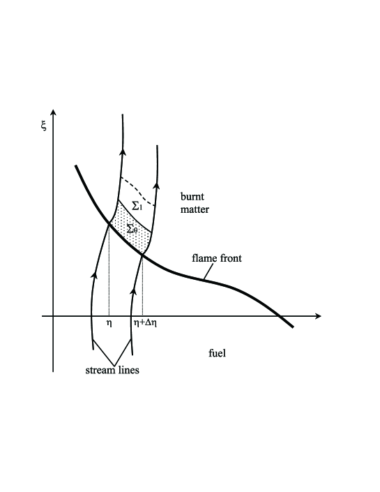
FIG. 1.: Elementary decomposition of the flow downstream.

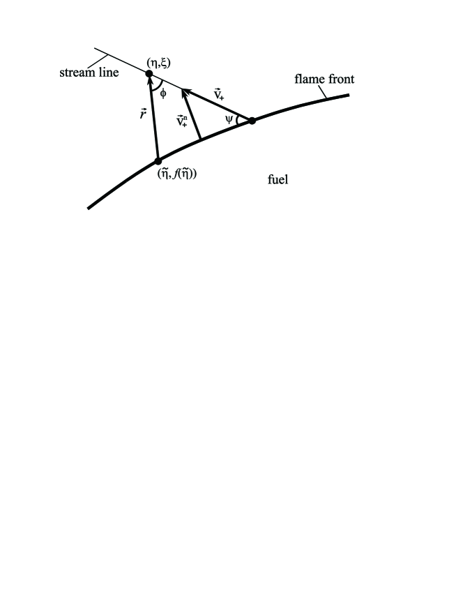
FIG. 2.: Near-the-front structure of the flow downstream. ${\bf v}^{n}_{+}={\bf n}v^{n}_{+}$ is the normal component of the velocity. Since the observation point $(\eta,\xi)$ is close to the flame front, the stream line and the part of the front near this point can be considered straight.

REFERENCES

- [1] G. I. Sivashinsky, “Nonlinear analysis of hydrodynamic instability in laminar flames,” Acta Astronaut. 4, 1177 (1977).
- [2] M. Matalon and B. J. Matkowsky, “Flames as gasdynamic discontinuities,” J. Fluid Mech. 124, 239 (1982).
- [3] P. Pelce and P. Clavin, “Influences of hydrodynamics and diffusion upon the stability limits of laminar premixed flames,” J. Fluid Mech. 124, 219 (1982).
- [4] G. I. Sivashinsky and P. Clavin, “On the nonlinear theory of hydrodynamic instability in flames,” J. Physique 48, 193 (1987).
- [5] K. A. Kazakov and M. A. Liberman, “Effect of vorticity production on the structure and velocity of curved flames,” Phys. Rev. Lett. 88, 064502 (2002).
- [6] K. A. Kazakov and M. A. Liberman, “Nonlinear equation for curved stationary flames,” Phys. Fluids 14, 1166 (2002).
- [7] L. D. Landau, “On the theory of slow combustion,” Acta Physicochimica URSS 19, 77 (1944).
- [8] G. Darrieus, unpublished work presented at La Technique Moderne, and at Le Congrs de Mcanique Applique, (1938) and (1945).
- [9] V. V. Bychkov, S. M. Golberg, M. A. Liberman, and L. E. Eriksson, “Propagation of curved stationary flames in tubes,” Phys. Rev. E 54, 3713 (1996).
- [10] K. A. Kazakov and M. A. Liberman, “Nonlinear theory of flame front instability,” E-print archive physics/0108057.
- [11] S. K. Zhdanov and B. A. Trubnikov, “Nonlinear theory of instability of a flame front,” J. Exp. Theor. Phys. 68, 65 (1989).