Structure Space of Model Proteins:
A Principal Component Analysis

Abstract

We study the space of all compact structures on a two-dimensional square lattice of size $N=6\times 6$. Each structure is mapped onto a vector in $N$-dimensions according to a hydrophobic model. Previous work has shown that the designabilities of structures are closely related to the distribution of the structure vectors in the $N$-dimensional space, with highly designable structures predominantly found in low density regions. We use principal component analysis to probe and characterize the distribution of structure vectors, and find a non-uniform density with a single peak. Interestingly, the principal axes of this peak are almost aligned with Fourier eigenvectors, and the corresponding Fourier eigenvalues go to zero continuously at the wave-number for alternating patterns ($q=\pi$). These observations provide a stepping stone for an analytic description of the distribution of structural points, and open the possibility of estimating designabilities of realistic structures by simply Fourier transforming the hydrophobicities of the corresponding sequences.

I INTRODUCTION

Proteins fold into specific structures to perform their biological function. Despite the huge diversity in their functions, evolutional paths, structural details, and sequences, the vast majority of proteins adopt only a small number ($\sim 1000$) of folds (“topology”). [1, 2, 3, 4, 5, 6] This observation has intrigued a number of authors and lead to the concept of designability. [1, 7, 8, 9, 10] The designability of a structure is defined to be the number of sequences that have that structure as their unique lowest-energy state. [10] It has been shown in various model studies that structures differ drastically in their designability; a small number of highly designable structures emerge with their associated number of sequences much larger than the average. [10, 11, 12, 13, 14, 15, 16] Highly designable structures are also found to possess other protein-like properties, such as thermodynamic stability, [10] fast folding kinetics, [9, 17] and tertiary symmetry. [8, 10, 18] These results suggest that there may be a designability principal behind nature’s selection of protein folds; these small number of folds were selected because they are readily designed, stable against mutations, and thermodynamically stable.

Why are some structures more designable than others? How do we identify highly designable structures? Finkelstein and co-workers argued that certain motifs are easier to stabilize and thus more common because they either have lower (e.g. bending) energies or have unusual energy spectra over random sequences. [1, 19, 20] Govindarajan and Goldstein suggested that the topology of a protein structure should be such that it is kinetically “foldable”. [9, 11, 21] More recently, it was noted that an important clue resides in the distribution of structures in a suitably defined structure space, with highly designable structures located in regions of low density. [12, 13] In particular, within a hydrophobic model, Li et al. showed that the distribution of structures is very nonuniform, and that the highly designable structures are those that are far away from other structures. [12] However, identifying highly designable structures still remains a tedious task, requiring either full enumeration or sufficiently large sampling of both the structure and the sequence spaces, making studies of large systems prohibitive.

In this paper, we investigate the properties of the structure space of the hydrophobic model of Li et al., starting from a Principal Component Analysis (PCA). We show that while the distribution of the structures is not uniform, it can be approximated as a cloud of points centered on a single peak. The principal directions of this cloud are almost coincident with those obtained by rotation into Fourier space; the coincidence is in fact exact for the subset of cyclic structures. An interesting feature is that the eigenvalues of PCA, describing the extent of the density cloud along the principal axis, vary continuously with the Fourier label $q$, with a minimum at $q=\pi$ corresponding to alternating patterns. The continuity of the eigenvalues suggests an expansion around $q=\pi$, which leads to an analytical conjecture for the density of structures in the $N$-dimensional binary space. Assuming the validity of this conjecture in more general models, it provides a means of estimating density, and hence indirectly designability, of structures by simply analyzing their sequences, without the need for extensive enumerations of other possible structures.

The rest of the paper is organized as follows. In Section II we review the hydrophobic model and the designabilities of structures. In Section III we discuss the methods and the results of PCA applied to the structure space, and relate the density and designability of a structure to its projections onto the principal axes. In Section IV we demonstrate that Fourier transformation provides a very good approximation to PCA, and show that in fact the two procedures are equivalent for the subset of cyclic structures. As a comparison with real structures, in Section V we introduce and study an ensemble of pseudo-structures constructed by a Markovian process. Finally, in Section VI we synthesize the numerical results of PCA analysis, and develop a conjecture for the density of points in structure space.

II THE HYDROPHOBIC MODEL

We start with a brief review of the hydrophobic model of Li et al. [12] and the designabilities of structures. Model sequences are composed of two types of amino acids, H and P. Each sequence $\{h_{i}\}$ (for $i=1,2,\cdots,N$) is represented by a binary string or vector, with $h_{i}=0$ for a P-mer and $h_{i}=1$ for an H-mer. We take the polymer length $N=36$, for which there are $2^{36}$ sequences. Each of these sequences can fold into any one of the many compact structures on a $6\times 6$ square lattice (Fig. 1). There are $57,337$ such compact structures unrelated by rotation and mirror symmetries. In the hydrophobic model, the only contribution to the energy for a sequence folded into a structure is the burial of the H-mers in the sequence into the core of the structure. So if one represents a structure by a binary string or vector, $\{s_{i}\}$, for $i=1,2,\cdots,36$, with $s_{i}=0$ for the surface sites and $s_{i}=1$ for the core sites (Fig. 1), the energy is

$$E=-\sum_{i=1}^{N}{h_{i}s_{i}},$$ (1)

where $h_{i}$ is the sequence vector.

The designability of a structure is defined as the number of sequences that have the structure as their unique lowest-energy state. To obtain an estimate for designabilities of structures, we randomly sampled $50,000,000$ sequences and found the unique lowest-energy structure, if any, for each of them. In Fig. 2, we plot the histogram of designabilities, i.e. number of structures with a given designability. Note that we have normalized designability so that its maximum value of $2981$ is scaled to one. In this paper, we define highly designable structures to be the top one percent of designable structures (structures with nonzero designability), which means $307$ structures with a designability larger than $0.47$.

In the hydrophobic model, both sequences and structures can be regarded as points in a 36-dimensional binary space, or corners of a hypercube in a Euclidean space of similiar dimension. In this representation, the lowest-energy state of a sequence is simply its nearest structure point. [12] Designabilities can then be obtained by constructing Voronoi polyhedra around all points corresponding to structures in this space; the designability of each structure is then the number of sequence points that fall within the corresponding Voronoi polytope (Fig. 3). Structures in the lower density regions have larger Voronoi polytopes and higher designability. Understanding how the structure points are distributed in this 36-dimensional space can thus help us address questions concerning designability. In the next section we examine the distribution of the structure points via the method of PCA.

III PRINCIPAL COMPONENT ANALYSIS

First, let us note that while sequences are uniformly distributed in the 36-dimensional hypercube, structures are distributed on a 34-dimensional hyperplane because of the following two geometrical constraints. The first constraint on structure vectors comes from the fact that all compact structures have the same number of core sites, and thus

$$\sum_{i=1}^{36}s_{i}=16.$$ (2)

The second constraint is that since the square lattice is bipartite, and any compact structure traverses an equal number of ‘black’ and ‘white’ points,

$$\sum_{i=1}^{36}(-1)^{i}s_{i}=0.$$ (3)

Next, let us define the covariance matrix of the structure space as

$$C_{i,j}=\left\langle s_{i}s_{j}\right\rangle-\left\langle s_{i}\right\rangle\left\langle s_{j}\right\rangle,$$ (4)

where $i,j=1,2,\cdots,36$, and the average is over all the $57,337$ possible $(s_{1},s_{2},\cdots,s_{36})$ for compact structures. The $36\times 36$ covariance matrix is symmetric $C_{i,j}=C_{j,i}$, and also satisfies the condition $C_{i,j}=C_{37-i,37-j}$. The latter is due to the reverse-labeling degeneracy of the structure ensemble, since if the string $(s_{1},s_{2},\cdots,s_{36})$ is in this ensemble, then its reverse $(s_{36},s_{35},\cdots,s_{1})$ is also included. This symmetry implies that if $(v_{1},v_{2},\cdots,v_{36})$ is an eigenvector of the matrix $C_{i,j}$, then $(v_{36},v_{35},\cdots,v_{1})$ is also an eigenvector with the same eigenvalue. Therefore, for every eigenvector of $C_{i,j}$ we have either $v_{j}=v_{37-j}$ or $v_{j}=-v_{37-j}$.

As depicted in Fig. 4, the matrix $C_{ij}$ is peaked along the diagonal and decays off-diagonally with short range correlations. This feature reflects a general property of compact self-avoiding walks; if a monomer is in the core (on the surface) the neighboring monomers along the chain have enhanced probability to be in the core (on the surface). Another characteristic of $C_{ij}$ is that it is almost a function of $|i-j|$ only, i.e. $C_{ij}\approx F(|i-j|)$, barring some small end and parity effects. We expect this feature of approximate translational invariance to be generic beyond the $6\times 6$ lattice model studied here. We also looked at the covariance matrix for the subset of highly designable structures. While qualitatively similar, it tends to decay faster off-diagonally than that of all structures. This is attributed to the fact that highly designable structures tend to have more frequent transitions between core and surface sites. [12, 15, 22]

For PCA of structure space, the matrix $C_{ij}$ is diagonalized to obtain its eigenvectors $\{\vec{v}\,^{(k)}\}$, and the corresponding eigenvalues $\{\lambda_{k}\}$ for $k=1,2,\cdots,36$, which are shown in Fig. 5. The two zero eigenvalues ($\lambda_{1}=\lambda_{2}=0$) result from the constraints in Eqs. (2) and (3), with the corresponding eigenvectors of $v_{i}^{(1)}=1$, and $v_{i}^{(2)}=(-1)^{i}$ for $i=1,2,\cdots,36$, respectively. The remaining 34 nonzero eigenvalues range smoothly from zero to one, making any further dimensional reduction not obvious. For comparison, the 36 eigenvalues of the uniformly distributed points of sequence space are all the same ($\lambda=1/4$). (It is easy to show that the covariance matrix for the sequence space is $C_{ij}=\delta_{ij}/4$.) On the other hand, a uniform distribution on the 34-dimensional hyperplane where the structure points reside would result in 34 identical eigenvalues of $360/1377\approx 0.26$.[23]

Identification of the principal axes and eigenvalues does not necessarily provide information about the distribution of points in space. To examine the latter, we first project each structure vector onto its components along the eigenvectors. Using the rotation matrix $R_{ki}$ that diagonalizes the covariance matrix, the component $y_{k}$ of the structure vector along principal axis $k$ is obtained as

$$y_{k}=\sum_{i=1}^{36}\left(s_{i}-\left\langle s_{i}\right\rangle\right)R_{ki}.$$ (5)

Interestingly, we find that along each of the principal directions, the distribution of components is a bell-shaped function with a single peak at zero. Such distributions can then be well approximated by Gaussians whose variances are the corresponding eigenvalues $\lambda_{k}$, i.e.

$$\rho_{k}(y_{k})\approx\frac{1}{\sqrt{2\pi\lambda_{k}}}e^{-\frac{y_{k}^{2}}{2\lambda_{k}}}.$$ (6)

In Fig. 6 we show the distribution of projections $y_{k}$ on two principal axes $k=16$ and $k=36$, along with the corresponding Gaussian distributions.

Equation (6) provides a good characterization of the density of structures in the $N$ dimensional space. Highly designable structures are expected to lie in regions of this space where the density of structures is small, while the number of available sequences is large. Let us consider a structure characterized by a vector $\vec{y}$. If the density of structural points in the vicinity of this point is $\rho_{str}({\vec{y}}\,)$, the number of available structures in a volume $V$ around this point is $V\rho_{str}({\vec{y}}\,)$. Neglecting various artifacts of discreteness, the volume of the Voronoi polyhedron (see Fig. 3) around this point is given by $V({\vec{y}}\,)\approx 1/\rho_{str}({\vec{y}}\,)$. The designability is the number of structures within this volume, and estimated as $\rho_{seq}({\vec{y}}\,)/\rho_{str}({\vec{y}}\,)$, where $\rho_{seq}({\vec{y}}\,)$ is the density of sequences. The sequence density is in fact uniform in the $N$-dimensional space. The structure density can be approximated as the product of Guassians along the principal projections, and thus

$${\rm Designability}\approx\frac{\rho_{seq}({\vec{y}}\,)}{\rho_{str}\left({\vec{y}}\,\right)}\propto\prod_{k=3}^{36}\frac{1}{\rho_{k}\left(y_{k}\right)}\propto\exp\left[\sum_{k=3}^{36}\frac{y_{k}^{2}}{2\lambda_{k}}\right]\equiv{\cal{M}}({\vec{y}}\,).$$ (7)

We have neglected various proportionality constants in the above equation, leading to the quantity ${\cal{M}}({\vec{y}}\,)$ which is our estimator for designability. In Fig. 7, the estimate $\cal{M}$ is plotted against the actual designability for all designable structures. There is a reasonably good, but by no means perfect, correlation between the designability and the estimator $\cal{M}$. The structures with the top one percent value of $\cal{M}$ include 39% of the highly designable structures.

IV FOURIER DECOMPOSITION AND CYCLIC STRUCTURES

In discussing Fig. 4, we already noted that the covariance matrix $C_{ij}$ is approximately a function of $|i-j|$, with corrections due to end effects. If this were an exact symmetry, the matrix would be diagonal in the Fourier basis. Even in the presence of the end effects, Fourier decomposition provides a very good approximation to the eigenvectors and eigenvalues of PCA, as demonstrated below. For each structure vector $\{s_{j}\}$, the Fourier components are obtained from

$$S_{q}={1\over\sqrt{N}}\sum_{j=1}^{N}e^{iqj}\left(s_{j}-\left\langle s_{j}\right\rangle\right),$$ (8)

where $q=2\pi\alpha/N$, with $\alpha=0,1,\cdots,N-1$. The average value of $\left\langle s_{j}\right\rangle$ is subtracted for convenience. With this subtraction, the two constraints in Eqs. (2) and (3) correspond to two zero modes in Fourier space, as $S_{0}=0$ and $S_{\pi}=0$, and since $\{s_{j}\}$ are real $S^{*}_{q}=S_{-q}$.

The covariance matrix in the Fourier space is

$$\left\langle S_{q}S^{*}_{q^{\prime}}\right\rangle={1\over N}\sum_{j,j^{\prime}=1}^{N}e^{i(qj-q^{\prime}j^{\prime})}C_{jj^{\prime}},$$ (9)

and is both real and symmetric (since $C_{jj^{\prime}}=C_{j^{\prime}j}$). If $C_{jj^{\prime}}$ is translationally invariant, i.e. $C_{jj^{\prime}}=F(|j-j^{\prime}|\bmod N)$, Eq. (9) becomes

$$\left\langle S_{q}S^{*}_{q^{\prime}}\right\rangle=\delta_{q,q^{\prime}}\lambda_{q},$$ (10)

where

$$\lambda_{q}=\sum_{k=0}^{N-1}e^{iqk}F(k)=\left\langle\left|S_{q}\right|^{2}\right\rangle,$$ (11)

are the diagonal elements of the diagonalized matrix in Eq. (10), and hence the eigenvalues of $C_{jj^{\prime}}$. Note that because the matrix is real–symmetric, its eigenvalues appear in pairs, i.e.

$$\lambda_{q}=\lambda_{-q}\,.$$ (12)

Since our covariance matrix is not fully translationally invariant, $\left\langle S_{q}S^{*}_{q^{\prime}}\right\rangle$ is not diagonal. However, as shown in Fig. 8a, its off diagonal elements are very small. As required by symmetry, the diagonal elements form pairs of identical values. These diagonal elements, plotted versus the index $\alpha$ in Fig. 8b, should provide a good approximation to the eigenvalues obtained by PCA. This is corroborated in Fig. 9a, where we compare $\left\langle|S_{q}|^{2}\right\rangle$ with the true eigenvalues of the covariance matrix $C_{jj^{\prime}}$.

Finally, we note that the end effects that mar the translational invariance of the covariance matrix are absent in the subset of cyclic structures. Any structure whose two ends are neighboring points on the lattice can be made cyclic by adding the missing bond. Any one of the $N=36$ bonds on the resulting closed loop can be broken to generate an element of the original set of structures, and the corresponding structure strings are cyclic permutations of each other. Thus, the covariance matrix $C_{cyclic}(j,j^{\prime})$ of the set of all cyclic structures is translationally invariant. In our model of $6\times 6$ compact polymers, there are a total of $36\times 276$ cyclic structures. The Fourier transform of their covaraince matrix is diagonal as expected, with diagonal elements depicted in Fig. 9b. The corresponding Fourier eigenvalues are quite close to the eigenvalues of the full matrix obtained in the PCA (Fig. 9b). Thus the end effects do not significantly modify the correlations, and this is specially true for the smallest eigenvalues which make the largest contributions to the density in Eq. 7.

V A MARKOVIAN ENSEMBLE of PSEUDO–STRUCTURES

The geometry of the lattice, and the requirement of compactness constrain the allowed structure strings of zeros and ones in a non-trivial fashion. In our estimation of designabilities so far, we have focused on the covariance matrix which carries information only about two point correlations along these strings. In principle, higher point correlations may also be important, and we may ask to what extent the covariance matrix contains the information about the structures’ designabilities? As a preliminary test, we performed a comparative study with an artificial set of strings, not corresponding to real structures, but constructed to have a covariance matrix similar to true structures on the $6\times 6$ lattice.

Specifically, we generated a set of random strings $\{\vec{t}\,\}$, of zeros and ones of length 36, using a third order Markov process as follows. For each string, the first element $t_{1}$ is generated with probability $P(t_{1}=1)=\left\langle s_{1}\right\rangle$, where $\left\langle s_{1}\right\rangle$ is the fraction of the true structure strings with $s_{1}=1$. The second element $t_{2}$ is generated according to a transition probability $P(t_{1}\to t_{2})$ which is taken to be the “conditional probability” $P(s_{2}|s_{1})$ extracted from the true structure strings. The third point $t_{3}$ is generated according to a transition probability $P(t_{1}t_{2}\to t_{3})$ which is the “conditional probability” $P(s_{3}|s_{1}s_{2})$ extracted from the true structure strings. All the remaining points $t_{j}$, $j=4,5,\cdots,36$, are generated according to the transition probabilities $P(t_{j-3}t_{j-2}t_{j-1}\to t_{j})$ equal to the true “conditional probabilities” $P(s_{j}|s_{j-3}s_{j-2}s_{j-1})$ of actual structures. Sequences that do not satisfy the global constrains of Eqs. (2) and (3) are thrown out. For every Markov string generated, we also put its reverse in the pool, unless the string is its own reverse.

The above Markovian ensemble has a covariance matrix, and corresponding eigenvalues, very similar to those of the true structures, as shown in Fig. 10. We then calculated the designabilities of these “pseudo-structures” using Eq. (1) by uniformly sampling $5\times 10^{7}$ random binary sequences. The histogram of the designabilities (Fig. 11) is qualitatively similar to that of the true structures (Fig. 2). Next we constructed the designability estimator $\cal{M}$ (Eq. (7)) for the pseudo-structures, using the eigenvalues and eigenvectors of their covariance matrix. The quantity $\cal{M}$ is plotted versus designability in Fig. 12 for all the artificial pseudo-structures with non-zero designability. The pseudo-structures with the top one percent value of $\cal{M}$ include 60% of the highly designable psuedo-structures.

These results suggest that a considerable amount of information about the designability is indeed contained in the two point correlations of the string. The designability estimator, Eq. (7) in fact does a somewhat better job in the case of pseudo-structures generated according to short-range Markov rules.

VI CONCLUSIONS

One of the most intriguing properties of compact structures, which emerged from early extensive enumeration studies,[10] is that designabilites range over quite a broad distribution of values. Such a large variation in designability is a consequence of a non-uniform distribution of structure vectors, with highly designable structures typically found in regions of low density.[12] However, our study of $6\times 6$ lattice structures using PCA indicates that the non-uniform density actually has a rather simple form that can be well approximated by a single multi-variable Gaussian, as in Eq. (7). Since this method of estimating structure designability is based only on the overall distribution of structures, it can be a useful tool in cases where there is not enough computational power to enumerate the whole structure space and calculate the designability. To obtain an accurate enough covariance matrix requires only a uniform sampling of the structure space.

We can also attempt to use the numerical results as a stepping stone to a more analytical approach for calculating the density of structures. First, we note that the covariance matrix for all structures is rather similar to that of the subset of cyclic structures, and that for the latter PCA is equivalent to Fourier decomposition. Second, we observe that the multi-variable Gaussian approximation to structure density in Eq. (7) is most sensitive to the eigenvalues that are close to zero. In terms of Fourier components, these are eigenvalues corresponding to values of $q$ close to $\pi$, and related to the constraint of Eq. (3). There is also a zero eigenvalue for $q=0$, related to condition (2). However, the latter global constraint appears not to have any local counterpart, as there is a discontinuity in the eigenvalues close to zero. Third, the continuity of the eigenvalues as $q\to\pi$, along with the symmetry of Eq. (12), suggests as expansion of the form $\lambda_{q}=K(q-\pi)^{2}+{\cal O}\left((q-\pi)^{4}\right)$. Indeed the numerical results indicate that the important (smaller) eigenvalues can well be approximated by $K(q-\pi)^{2}$, with $K\approx 0.04$.[24]

With this approximation, the designability estimate of Eq. (7) becomes

$${\cal{M}}\left(\left\{\vec{s}\,\right\}\right)\approx\exp\left[\sum_{q}\frac{\left|S_{q}\right|^{2}}{2K(q-\pi)^{2}}\right]=\exp\left[\frac{1}{2K}\sum_{i,j=1}^{N}(-1)^{i}s_{i}J_{N}\left(|i-j|\right)(-1)^{j}s_{j}\right].$$ (13)

The first form in the above equation expresses the estimate in terms of the Fourier modes of the structure string, while the second term is directly in terms of the elements $\{s_{i}\}$. The function $J_{N}\left(|i-j|\right)$ is the discrete Fourier transform of $1/q^{2}$, which for large $N$ behaves as $|i-j|$. Equation (13) is thus equivalent to the Boltzmann weight of a set of unit charges on a discrete line of $N$ points marked by parity. The charges on the sublattice of the same parity attract each other with a potential $J_{N}(r)$, while those on different sublattices repel. Such an interaction gives a larger weight (and hence designability) to configurations in which the charges alternate between the core and surface sites, as observed empirically.[12, 15, 22]

In would be revealing to see how much of the above results, developed on the basis of a lattice hydrophobic model, can be applied to real protein structures. One could use the exposure level of residues to the solvent in building up the structure vectors. Current methods deal with structure strings of a fixed length, equal to the dimension of the structure space. Since real proteins have different lengths, there is a need for a scaling method to handle them all together. Our study shows that the two point correlations of structure vectors are approximately translationally invariant, and can be captured by Fourier analysis. This suggests the possibility of casting the density of points in structure space in universal functional forms dependent only of a few parameters encoding the properties of the underlying polymers. If so, it would be possible to provide good estimates for designability with polymers of varying length, without the need for extensive numerical computations.

VII ACKNOWLEDGEMENT

We thank G. Gatz, N. Butchler and E. Domany for useful discussions. The work was initiated, and partly completed, during the Program on Statistical Physics and Biological Information at the Institute for Theoretical Physics, UCSB, supported in part by the NSF Contract No. PHY99-07949. We acknowledge support by the NSF Grant No. DMR-01018213 (MY and MK), and an ITP Graduate Fellowship (MY).

FIGURE CAPTIONS

1. A possible compact structure on the $6\times 6$ square lattice. The 16 sites in the core region, enclosed by the dashed lines, are indicated by 1’s; the 20 sites on the surface are labeled by 0’s. Hence this structure is represented by the string 001100110000110000110011000011111100. Note that each ‘undirected’ open geometrical structure can be represented by two ‘directed’ strings, starting from its two possible ends (except for structures with reverse-labeling symmetry where the two strings are identical). It is also possible for the same string to represent different structures which are folded differently in the core region. For the $6\times 6$ lattice of this study, there are $26929$ such ‘degenerate’ structures, which are by definition non-designable.

2. Number of structures with a given designability versus relative designability for the $6\times 6$ hydrophobic model. The data is generated by uniformly sampling $5\times 10^{7}$ strings from the sequence space. The designability of each structure is normalized by the maximum possible designability.

3. Schematic representation of the 36-dimensional space in which sequences and structures are vectors or points. Sequences, represented by dots, are uniformly distributed in this space. Structures, represented by circles, occupy only a sparse subset of the binary points and are distributed non-uniformly. The sequences lying closer to a particular structure than to any other, have that structure as their unique ground state. The designability of a structure is therefore the number of sequences lying entirely within the Voronoi polytope about that structure.

4. Covariance matrix $C_{ij}$ of all compact structures of the $6\times 6$ square.

5. Eigenvalues of the covariance matrix for the structure vectors (circles), and for all points in sequence space (crosses).

6. Distributions of projections $y_{k}$ onto principal axes $k=16$ (a), and $k=36$ (b), for all 57337 structures (dots). Also plotted are Gaussian forms with variances $\lambda_{16}$ and $\lambda_{36}$, respectively (dashed lines).

7. The estimate $\cal{M}$ (Eq. (7)) versus scaled designability for all designable structures on the $6\times 6$ square.

8. (a) The Fourier transformed covariance matrix $\left\langle S_{q}S^{*}_{q^{\prime}}\right\rangle$ (Eq. (9)); and (b) its diagonal elements $\left\langle|S_{q}|^{2}\right\rangle$.

9. (a)The diagonal elements $\left\langle|S_{q}|^{2}\right\rangle$ (dots) plotted together with the eigenvalues of the covariance matrix (pluses). (b) Diagonal elements of the Fourier transformed $C_{cyclic}$, which are also the eigenvalues of the covariance matrix of cyclic structures (pluses). Eigenvalues of the covariance matrix for all structures are indicated by stars.

10. Eigenvalues of the covariance matrix for the structures generated by the Markov model (circles), and that of the true structure space (pluses).

11. Number of pseudo-structures with a given designability versus designability for the pseudo-structure strings randomly generated using the Markov model. The data is generated by uniformly sampling $5\times 10^{7}$ binary sequence strings. The designability of each pseudo-structure is normalized by the maximum possible designability.

12. The quantity $\cal{M}$ versus designability for all designable pseudo-structures generated by the Markov model.

FIG. 1.: Yahyanejad, et al.

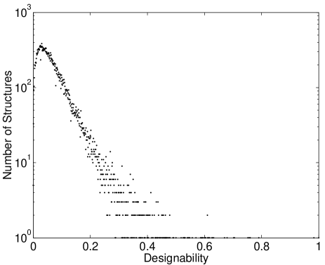
FIG. 2.: Yahyanejad, et al.

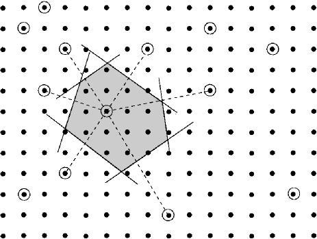
FIG. 3.: Yahyanejad, et al.

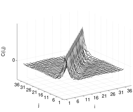
FIG. 4.: Yahyanejad, et al.

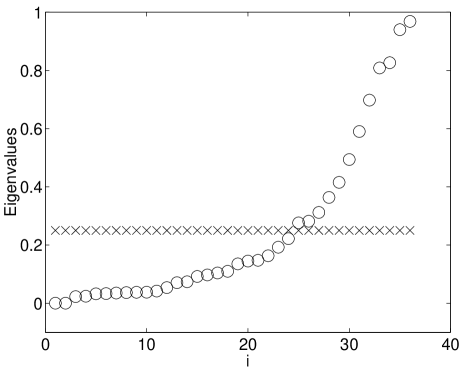
FIG. 5.: Yahyanejad, et al.

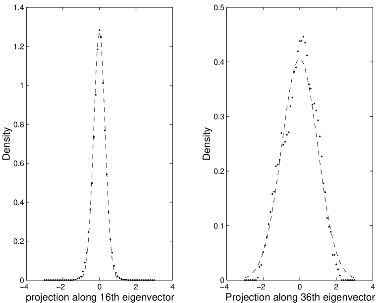
FIG. 6.: Yahyanejad, et al.

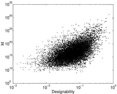
FIG. 7.: Yahyanejad, et al.

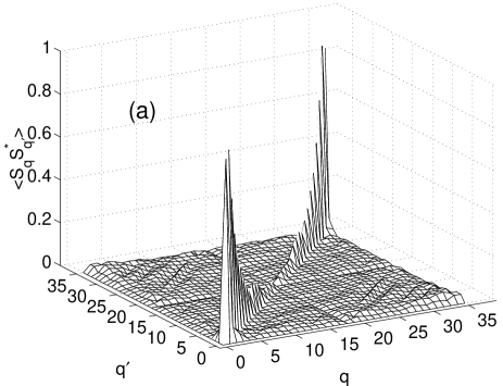
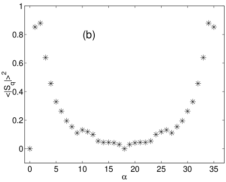
FIG. 8.: Yahyanejad, et al.

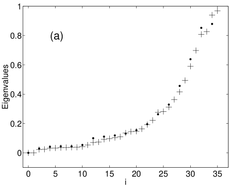
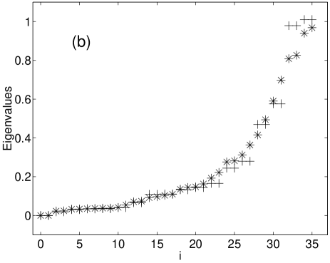
FIG. 9.: Yahyanejad, et al.

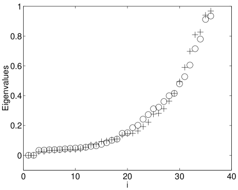
FIG. 10.: Yahyanejad, et al.

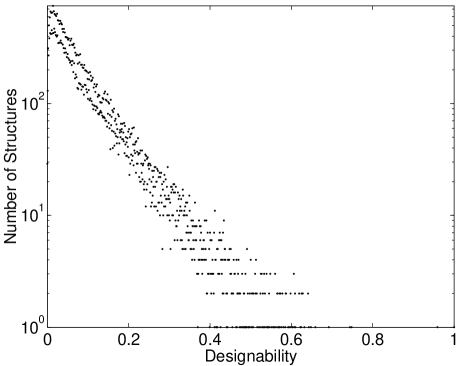
FIG. 11.: Yahyanejad, et al.

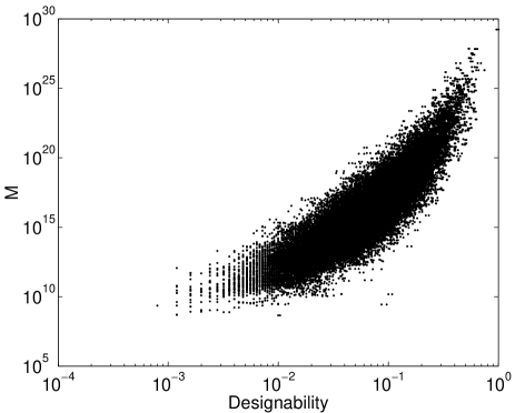
FIG. 12.: Yahyanejad, et al.

REFERENCES

- [1] A. V. Finkelstein and O. B. Ptitsyn, Prog. Biophys. Mol. Biol. 50, 171 (1987).
- [2] C. Chothia, Nature 357, 543 (1992).
- [3] S. E. Brenner, C. Chothia, and T. J. P. Hubbard, Curr. Opin. in Struct. Biol. 7, 369 (1997).
- [4] C. A. Orengo, D. T. Jones, and J. M. Thornton, Nature 372, 631 (1994).
- [5] Z. X. Wang, Proteins 26, 186 (1996).
- [6] S. Govindarajan, R. Recabarren, and R. A. Goldstein, Proteins 35, 408 (1999).
- [7] C. J. Camacho and D. Thirumalai, Phys. Rev. Lett. 71, 2505 (1993).
- [8] K. Yue and K. A. Dill, Proc. Natl. Acad. Sci. USA 92, 146 (1995).
- [9] S. Govindarajan and R. A. Goldstein, Biopolymers 36, 43 (1995).
- [10] H. Li, R. Helling, C. Tang, and N. S. Wingreen, Science 273, 666 (1996).
- [11] S. Govindarajan and R. A. Goldstein, Proc. Natl. Acad. Sci. USA 93, 3341 (1996).
- [12] H. Li, C. Tang, and N. S. Wingreen, Proc. Natl. Acad. Sci. USA 95, 4987 (1998).
- [13] N. E. G. Buchler and R. A. Goldstein, J. Chem. Phys. 112, 2533 (2000).
- [14] R. Helling, H. Li, J. Miller, R. Mélin, N. Wingreen, C. Zeng, and C. Tang, J. Mol. Graph. Model. 19, 157 (2001).
- [15] H. Cejtin, J. Edler, A. Gottlieb, R. Helling, H. Li, J. Philbin, N. Wingreen, and C. Tang, J. Chem. Phys. 116, 352 (2002).
- [16] J. Miller, C. Zeng, N.S. Wingreen, and C. Tang, Proteins 47, 506 (2002).
- [17] R. Mélin, H. Li, N. Wingreen, and C. Tang, J. Chem. Phys. 110, 1252 (1999).
- [18] T. Wang, J. Miller, N. Wingreen, C. Tang, and K. Dill, J. Chem. Phys. 113, 8329 (2000).
- [19] A. V. Finkelstein, A. M. Gutin, and A. Y. Badretdinov, FEBS Lett. 325, 23 (1993).
- [20] A. V. Finkelstein, A. Y. Badretdinov, and A. M. Gutin, Proteins 23, 142 (1995).
- [21] S. Govindarajan and R. A. Goldstein, Biopol. 42, 427 (1997).
- [22] C. T. Shih, Z. Y. Su, J. F. Gwan, B. L. Hao, C. H. Hsieh, and H. C. and Lee, Phys. Rev. Lett. 84, 386 (2000).
- [23] This can be seen from the following argument: Since all points in the 34-dimensional hyperplane are equivalent up to parity, the most general form of the covariance matrix is . Requiring zero eigenvalues for eigenvectors and gives the constraints , and , i.e. . The value of is then set by , where . So we have and . It is then easy to see that the 34 nonzero eigenvalues are .
- [24] If not forced to go through zero for , a somewhat better fit can be obtained with . Fourier transforming back to real space, the additional constant leads to screened Coulomb interactions for .