Nuclear-polarization correction to the bound-electron $g$ factor in heavy hydrogenlike ions

Abstract

The influence of nuclear polarization on the bound-electron $g$ factor in heavy hydrogenlike ions is investigated. Numerical calculations are performed for the K- and L-shell electrons taking into account the dominant virtual nuclear excitations. This determines the ultimate limit for tests of QED utilizing measurements of the bound-electron $g$ factor in highly charged ions.

Recent high-precision experiments for measuring the bound-electron $g$ factor in hydrogenlike carbon have reached a level of accuracy of about $2\times 10^{-9}$ [1, 2]. As a consequence, this has led to a new independent determination of the electron mass [3]. Via investigations of the $g$ factor of a bound electron in a highly charged ion one can probe nontrivial effects in bound-state QED as sensitive as in high-precision Lamb shift experiments. A further improvement in accuracy and the extension to systems with higher nuclear charge numbers $Z$ up to hydrogenlike uranium is intended in the near future [1]. Studies of $g$ factors in heavy ions are of particular importance, since they can provide a possibility for an independent determination of the fine-structure constant [4, 5], nuclear magnetic moments [5], and nuclear charge radii. In order to achieve a level of utmost precision in corresponding theoretical calculations, one has to account for the relativistic, higher-order QED, nuclear-size, nuclear-recoil, and nuclear-polarization corrections [6, 7, 8, 9, 10, 11, 12, 13, 14]. Investigations of QED effects in heavy systems are strongly restricted by the uncertainty due to the finite nuclear size [8, 14]. In Ref. [15], a specific difference has been introduced for bound-electron $g$ factors in H- and Li-like ions, for which the uncertainty due to the nuclear-size effect can be significantly reduced. With an apparent accuracy of $10^{-9}$ for the bound-electron $g$ factor one could probe higher-order QED corrections even for uranium ions, provided that nuclear polarization effects remain negligible.

In the present Letter, we evaluate nuclear-polarization corrections to the $g$ factor in hydrogenlike ions. This reduces the remaining source of uncertainties in the prediction of nuclear effects. Moreover, we determine the ultimate limit of accuracy for QED tests in measurements of the bound-electron $g$ factor in highly charged ions.

We consider a hydrogenlike ion with a spinless nucleus, which is placed in a homogeneous external magnetic field $\textstyle\cal H$ corresponding to a vector potential $\mathchoice{{\hbox{\boldmath$\displaystyle A$}}}{{\hbox{\boldmath$\textstyle A$}}}{{\hbox{\boldmath$\scriptstyle A$}}}{{\hbox{\boldmath$\scriptscriptstyle A$}}}(\mathchoice{{\hbox{\boldmath$\displaystyle r$}}}{{\hbox{\boldmath$\textstyle r$}}}{{\hbox{\boldmath$\scriptstyle r$}}}{{\hbox{\boldmath$\scriptscriptstyle r$}}})=[\mathchoice{{\hbox{\boldmath$\displaystyle\cal H$}}}{{\hbox{\boldmath$\textstyle\cal H$}}}{{\hbox{\boldmath$\scriptstyle\cal H$}}}{{\hbox{\boldmath$\scriptscriptstyle\cal H$}}}\times\mathchoice{{\hbox{\boldmath$\displaystyle r$}}}{{\hbox{\boldmath$\textstyle r$}}}{{\hbox{\boldmath$\scriptstyle r$}}}{{\hbox{\boldmath$\scriptscriptstyle r$}}}]/2$. The energy shift of a bound-electron level $a$ within first-order perturbation theory in the magnetic field (see Fig. 1(a)) is given by ($\hbar=c=1$)

$$\Delta E_{a}=\langle\psi_{a}|V_{\cal H}|\psi_{a}\rangle,$$ (1)

where

$$V_{\cal H}=\frac{|e|}{2}(\mathchoice{{\hbox{\boldmath$\displaystyle\cal H$}}}{{\hbox{\boldmath$\textstyle\cal H$}}}{{\hbox{\boldmath$\scriptstyle\cal H$}}}{{\hbox{\boldmath$\scriptscriptstyle\cal H$}}}\cdot[\mathchoice{{\hbox{\boldmath$\displaystyle r$}}}{{\hbox{\boldmath$\textstyle r$}}}{{\hbox{\boldmath$\scriptstyle r$}}}{{\hbox{\boldmath$\scriptscriptstyle r$}}}\times\mathchoice{{\hbox{\boldmath$\displaystyle\alpha$}}}{{\hbox{\boldmath$\textstyle\alpha$}}}{{\hbox{\boldmath$\scriptstyle\alpha$}}}{{\hbox{\boldmath$\scriptscriptstyle\alpha$}}}]).$$ (2)

Choosing the $z$ axis along the direction of the field $\textstyle\cal H$, i.e., $\mathchoice{{\hbox{\boldmath$\displaystyle\cal H$}}}{{\hbox{\boldmath$\textstyle\cal H$}}}{{\hbox{\boldmath$\scriptstyle\cal H$}}}{{\hbox{\boldmath$\scriptscriptstyle\cal H$}}}=(0,0,{\cal H})$, one obtains for the energy shift

$$\Delta E_{a}=\mu_{0}{\cal H}m_{j}g_{a},$$ (3)

where $\mu_{0}=|e|/(2m)$ is the Bohr magneton, $m_{j}$ is the $z$-projection of the total angular momentum, and $g_{a}$ is the bound-electron $g$ factor, which depends on the electron configuration. In the case of a Dirac electron in the Coulomb field of an infinitely heavy point-like nucleus, it yields [16]

$$g^{\rm D}_{n\kappa}=\frac{\kappa}{j(j+1)}\left(\kappa\frac{\varepsilon_{n\kappa}}{m}-\frac{1}{2}\right).$$ (4)

Here $\kappa=(j+1/2)(-1)^{j+l+1/2}$ is the relativistic angular-momentum quantum number, $j$ is the total angular momentum of the electron, $l=j\pm 1/2$ defines the parity of the state, $\varepsilon_{n\kappa}$ is the one-electron energy of the state given by

$$\varepsilon_{n\kappa}=m\frac{\gamma+n_{r}}{N},$$ (5)

where $n_{r}=n-|\kappa|$ is the radial quantum number, $n$ is the principal quantum number, $\gamma=\sqrt{\kappa^{2}-(\alpha Z)^{2}}$, $N=\sqrt{(n_{r}+\gamma)^{2}+(\alpha Z)^{2}}$, and $\alpha=e^{2}$ is the fine-structure constant. Due to various QED and nuclear effects, the observed bound-electron $g$ factor deviates from its Dirac value (4). Here we consider the nuclear-polarization correction $\Delta g_{n\kappa}$, which is of particular importance in heavy ions.

The dominant contribution to the nuclear-polarization effect for heavy nuclei arises from virtual collective nuclear excitations. Three types of collective modes should be taken into account: (a) rotations of the deformed nuclei; (b) harmonic surface vibrations; and (c) giant resonances. In Ref. [17], a relativistic field theoretical approach has been developed, where the nuclear-polarization effects are treated perturbatively, incorporating the many-body theory for virtual nuclear excitations within bound-state QED for atomic electrons. The contribution of the nuclear vector current can be omitted, because the velocities associated with collective nuclear dynamics are nonrelativistic [18]. Accordingly, one is left with the longitudinal component of the effective photon propagator $D_{00}$ only due to the nuclear transition density-correlation function. In Coulomb gauge, it can be represented in terms of a multipole decomposition as follows [17]

$$D_{00}(\mathchoice{{\hbox{\boldmath$\displaystyle r$}}}{{\hbox{\boldmath$\textstyle r$}}}{{\hbox{\boldmath$\scriptstyle r$}}}{{\hbox{\boldmath$\scriptscriptstyle r$}}},\mathchoice{{\hbox{\boldmath$\displaystyle r$}}}{{\hbox{\boldmath$\textstyle r$}}}{{\hbox{\boldmath$\scriptstyle r$}}}{{\hbox{\boldmath$\scriptscriptstyle r$}}}^{\prime};\omega)=\sum_{L\geq 0}B(EL)\frac{2\omega_{L}}{2L+1}\frac{F_{L}(r)F_{L}(r^{\prime})}{\omega^{2}-\omega_{L}^{2}+i0}(\mathchoice{{\hbox{\boldmath$\displaystyle Y$}}}{{\hbox{\boldmath$\textstyle Y$}}}{{\hbox{\boldmath$\scriptstyle Y$}}}{{\hbox{\boldmath$\scriptscriptstyle Y$}}}_{L}(\Omega)\cdot\mathchoice{{\hbox{\boldmath$\displaystyle Y$}}}{{\hbox{\boldmath$\textstyle Y$}}}{{\hbox{\boldmath$\scriptstyle Y$}}}{{\hbox{\boldmath$\scriptscriptstyle Y$}}}_{L}(\Omega^{\prime})).$$ (6)

Here $\omega_{L}=E_{L}-E_{0}$ are the nuclear excitation energies with respect to the ground-state energy $E_{0}$ of the nucleus and $B(EL)=B(EL;0\to L)$ are the corresponding reduced electric transition probabilities. The radial shape parametrizing the nuclear transitions is carried by the functions

$$F_{L}(r)=\frac{4\pi}{(2L+1)R_{0}^{L}}\left[\frac{r^{L}}{R_{0}^{L+1}}\Theta(R_{0}-r)+\frac{R_{0}^{L}}{r^{L+1}}\Theta(r-R_{0})\right]$$ (7)

for the case of multipole excitations with $L\geq 1$ and

$$F_{0}(r)=\frac{5\sqrt{\pi}}{2R_{0}^{3}}\left[1-\left(\frac{r}{R_{0}}\right)^{2}\right]\Theta(R_{0}-r)$$ (8)

for monopole excitations, respectively. Here $R_{0}$ is an average radius assigned to the nucleus in its ground state. The presence of $\Theta$-functions in the expressions (7) and (8) reflects the sharp surface approximation for collective excitations. The form (6) of the propagator is convenient for numerical evaluations, since the parameters characterizing the nuclear dynamics $\omega_{L}$ and $B(EL)$ can be taken from experiment. Nuclear-polarization corrections to the Lamb shift (see graph on Fig. 1(b)) have been calculated in Refs. [17, 18, 19, 20].

The nuclear-polarization contribution to the bound-electron $g$ factor appears as the lowest-order nuclear-polarization correction to the diagram 1(a). To first order in $V_{\cal H}$, this perturbation gives rise to a modification of the wave function, of the binding energy, and of the electron propagator. The corresponding contributions are referred to as the irreducible part, the reducible part, and the vertex part, respectively. The nuclear-polarization energy shift of the state under consideration may be represented by the diagrams depicted in Figs. 1(c) and 1(d). Let us consider first the energy correction due to the irreducible part of the graph  1(c)

$$\Delta E_{a}^{\rm irr} = -2\alpha\sum_{L,M}B(EL)\frac{2\omega_{L}}{2L+1}\sum_{n,k}^{\varepsilon_{k}\neq\varepsilon_{a}}\int\limits_{-\infty}^{+\infty}\frac{d\omega}{2\pi i}\frac{\langle\psi_{a}|F_{L}Y_{LM}|\psi_{n}\rangle}{\varepsilon_{a}-\omega-\varepsilon_{n}(1-i0)}$$ (9)

$$\times \frac{\langle\psi_{n}|F_{L}Y^{*}_{LM}|\psi_{k}\rangle}{\omega^{2}-\omega^{2}_{L}+i0}\frac{\langle\psi_{k}|V_{\cal H}|\psi_{a}\rangle}{\varepsilon_{a}-\varepsilon_{k}(1-i0)}.$$ (10)

Here the indices $n$ and $k$ in the sum run over the entire Dirac spectrum.

After integration over frequencies $\omega$ and summation over angular projections, Eq. (10) takes the form

$$\Delta E_{n\kappa}^{\rm irr} = \mu_{0}{\cal H}m_{j}\frac{\alpha}{2\pi}\frac{\kappa m}{j(j+1)}\sum_{L}B(EL)\sum_{n_{1},\kappa_{1}}\sum_{n_{2}}^{n_{2}\neq n}\left[C^{j_{1}\frac{1}{2}}_{j\frac{1}{2}L0}\right]^{2}$$ (11)

$$\times \frac{\langle n\kappa|F_{L}|n_{1}\kappa_{1}\rangle\langle n_{1}\kappa_{1}|F_{L}|n_{2}\kappa\rangle}{\varepsilon_{n\kappa}-\varepsilon_{n_{1}\kappa_{1}}-{\rm sgn}(\varepsilon_{n_{1}\kappa_{1}})\omega_{L}}\frac{\langle n_{2}\kappa|r\sigma_{x}|n\kappa\rangle}{\varepsilon_{n\kappa}-\varepsilon_{n_{2}\kappa}}.$$ (12)

The sum over $\kappa_{1}$ is restricted to those intermediate states, where $l+l_{1}+L$ is even. In Eq. (12), a two-component radial vector $\langle r|n\kappa\rangle$ is determined by

$$\langle r|n\kappa\rangle={{P_{n\kappa}(r)}\choose{Q_{n\kappa}(r)}},$$ (13)

where $P_{n\kappa}(r)=rg_{n\kappa}(r)$ and $Q_{n\kappa}(r)=rf_{n\kappa}(r)$, with $g_{n\kappa}(r)$ and $f_{n\kappa}(r)$ being the upper and lower radial components of the Dirac wave function [21], respectively. The radial matrix element is given by

$$\langle a|F_{L}|b\rangle=\int\limits_{0}^{\infty}drF_{L}(r)\left[P_{a}(r)P_{b}(r)+Q_{a}(r)Q_{b}(r)\right]$$ (14)

and $\sigma_{x}$ denotes the Pauli matrix. The sum

$$\langle r|\overline{n\kappa}\rangle=\sum_{n^{\prime}}^{n^{\prime}\neq n}\frac{\langle r|n^{\prime}\kappa\rangle\langle n^{\prime}\kappa|r\sigma_{x}|n\kappa\rangle}{\varepsilon_{n\kappa}-\varepsilon_{n^{\prime}\kappa}}$$ (15)

can be evaluated analytically using the generalized virial relations for the Dirac equation [22]. The upper and lower components $\overline{P}_{n\kappa}(r)$ and $\overline{Q}_{n\kappa}(r)$ of the vector $\langle r|\overline{n\kappa}\rangle$ read [10]

$$\overline{P}_{n\kappa}(r) = \frac{1}{m^{2}}\left[\left(m\kappa-\frac{m}{2}+\kappa\varepsilon_{n\kappa}\right)r+\alpha Z\kappa\right]Q_{n\kappa}(r)+\frac{\kappa}{2m^{2}}(1-2\kappa)P_{n\kappa}(r),$$ (16)

$$\overline{Q}_{n\kappa}(r) = \frac{1}{m^{2}}\left[\left(m\kappa+\frac{m}{2}-\kappa\varepsilon_{n\kappa}\right)r-\alpha Z\kappa\right]P_{n\kappa}(r)+\frac{\kappa}{2m^{2}}(1+2\kappa)Q_{n\kappa}(r).$$ (17)

Finally, the corresponding irreducible part of the correction $\Delta g_{n\kappa}$ can be expressed as

$$\Delta g^{\rm irr}_{n\kappa}=\frac{\alpha}{2\pi}\frac{\kappa m}{j(j+1)}\sum_{L}B(EL)\sum_{n_{1},\kappa_{1}}\left[C^{j_{1}\frac{1}{2}}_{j\frac{1}{2}L0}\right]^{2}\frac{\langle n\kappa|F_{L}|n_{1}\kappa_{1}\rangle\langle n_{1}\kappa_{1}|F_{L}|\overline{n\kappa}\rangle}{\varepsilon_{n\kappa}-\varepsilon_{n_{1}\kappa_{1}}-{\rm sgn}(\varepsilon_{n_{1}\kappa_{1}})\omega_{L}}.$$ (18)

The reducible part of the graph depicted in Fig. 1(c) has to be considered together with the contributions resulting from diagrams 1(a) and 1(b). The corresponding corrections to the energy shift reads

$$\Delta E_{a}^{\rm red} = \alpha\langle\psi_{a}|V_{\cal H}|\psi_{a}\rangle\sum_{L,M}B(EL)\frac{2\omega_{L}}{2L+1}\sum_{n}\int\limits_{-\infty}^{+\infty}\frac{d\omega}{2\pi i}\frac{\langle\psi_{a}|F_{L}Y_{LM}|\psi_{n}\rangle}{\omega^{2}-\omega^{2}_{L}+i0}$$ (19)

$$\times \frac{\langle\psi_{n}|F_{L}Y_{LM}^{*}|\psi_{a}\rangle}{[\varepsilon_{a}-\omega-\varepsilon_{n}(1-i0)]^{2}},$$ (20)

leading to the $g$-factor correction

$$\Delta g^{\rm red}_{n\kappa}=-\frac{\alpha}{4\pi}g^{\rm D}_{n\kappa}\sum_{L}B(EL)\sum_{n_{1},\kappa_{1}}\frac{\left[C^{j_{1}\frac{1}{2}}_{j\frac{1}{2}L0}\right]^{2}\langle n\kappa|F_{L}|n_{1}\kappa_{1}\rangle{}^{2}}{[\varepsilon_{n\kappa}-\varepsilon_{n_{1}\kappa_{1}}-{\rm sgn}(\varepsilon_{n_{1}\kappa_{1}})\omega_{L}]^{2}}.$$ (21)

Here $g^{\rm D}_{n\kappa}$ is the Dirac $g$ factor given by Eq. (4). In Eqs. (18) and (21), the sum $l+l_{1}+L$ again should be even.

Let us now turn to the nuclear-polarization correction to the vertex as depicted in Fig. 1(d). The corresponding energy shift is determined by

$$\Delta E_{a}^{\rm ver} = -\alpha\sum_{L,M}B(EL)\frac{2\omega_{L}}{2L+1}\sum_{n,k}\int\limits_{-\infty}^{+\infty}\frac{d\omega}{2\pi i}\frac{\langle\psi_{a}|F_{L}Y_{LM}|\psi_{n}\rangle}{\varepsilon_{a}-\omega-\varepsilon_{n}(1-i0)}$$ (22)

$$\times \frac{\langle\psi_{n}|V_{\cal H}|\psi_{k}\rangle}{\omega^{2}-\omega^{2}_{L}+i0}\frac{\langle\psi_{k}|F_{L}Y^{*}_{LM}|\psi_{a}\rangle}{\varepsilon_{a}-\omega-\varepsilon_{k}(1-i0)}.$$ (23)

The integration over $\omega$ and the summation over angular variables leads to the corresponding expression for $\Delta g^{\rm ver}_{n\kappa}$, which is conveniently represented as the sum of a pole term

$$\Delta g^{\rm pol}_{n\kappa} = \frac{\alpha}{4\pi}\frac{\kappa m}{\sqrt{j(j+1)(2j+1)}}\sum_{L}B(EL)\sum_{n_{1},\kappa_{1}}\frac{(2j_{1}+1)^{3/2}}{\sqrt{j_{1}(j_{1}+1)}}\left[C^{j_{1}\frac{1}{2}}_{j\frac{1}{2}L0}\right]^{2}\left\{{j_{1}\atop j}{j_{1}\atop j}{1\atop L}\right\}$$ (24)

$$\times \frac{\langle n_{1}\kappa_{1}|r\sigma_{x}|n_{1}\kappa_{1}\rangle\langle n\kappa|F_{L}|n_{1}\kappa_{1}\rangle{}^{2}}{[\varepsilon_{n\kappa}-\varepsilon_{n_{1}\kappa_{1}}-{\rm sgn}(\varepsilon_{n_{1}\kappa_{1}})\omega_{L}]^{2}}$$ (25)

and of a residual term

$$\Delta g^{\rm res}_{n\kappa} = \frac{\alpha}{\pi}\frac{2\kappa m}{\sqrt{j(j+1)(2j+1)}}\sum_{L}B(EL)\mathop{{\sum}^{\prime}}_{n_{1},n_{2}}\sum_{\kappa_{1},\kappa_{2}}\sqrt{j_{2}+1/2}C^{j_{1}\frac{1}{2}}_{j\frac{1}{2}L0}C^{j_{2}\frac{1}{2}}_{j\frac{1}{2}L0}C^{j_{1}\frac{1}{2}}_{j_{2}-\frac{1}{2}11}$$ (26)

$$\times \left\{{j_{1}\atop j}{j_{2}\atop j}{1\atop L}\right\}\frac{\langle n\kappa|F_{L}|n_{1}\kappa_{1}\rangle\langle n_{2}\kappa_{2}|F_{L}|n\kappa\rangle}{\varepsilon_{n\kappa}-\varepsilon_{n_{2}\kappa_{2}}-{\rm sgn}(\varepsilon_{n_{2}\kappa_{2}})\omega_{L}}\frac{\langle n_{1}\kappa_{1}|r\sigma_{x}|n_{2}\kappa_{2}\rangle}{\varepsilon_{n_{1}\kappa_{1}}-\varepsilon_{n_{2}\kappa_{2}}},$$ (27)

respectively. Here $\Delta g^{\rm pol}_{n\kappa}$ accounts for the terms with $n_{1}=n_{2}$ and $\kappa_{1}=\kappa_{2}$ in the sums over intermediate states. The prime in the sum in Eq. (27) indicates that $\varepsilon_{n_{1}\kappa_{1}}\neq\varepsilon_{n_{2}\kappa_{2}}$ when $\kappa_{1}=\kappa_{2}$, i.e., the pole contribution is supposed to be omitted. In Eqs. (25) and (27), the value $l+l_{1}+L$ has to be even. A second condition in Eq. (27) is that the sum $l_{1}+l_{2}$ should be even as well. The total nuclear-polarization contribution to the $g$ factor is determined by the sum of all contributions given by Eqs. (18), (21), (25), and (27).

We have evaluated the nuclear-polarization correction to the $g$ factor taking into account a finite set of dominant collective nuclear excitations (see Table I). For low-lying rotational and vibrational levels, the corresponding nuclear parameters, $\omega_{L}$ and $B(EL)$, have been taken from experiments on nuclear Coulomb excitation. In our estimates for the contributions due to giant resonances, we utilized phenomenological energy-weighted sum rules [20, 23]. The latter are assumed to be concentrated in single resonant states. In the present calculations, contributions due to monopole, dipole, quadrupole, and octupole giant resonances have been taken into account. To evaluate the infinite summations over the entire Dirac spectrum, the finite basis set method has been employed. Basis functions have been generated via B splines including nuclear-size effects [24]. The major contribution to the $\Delta g_{n\kappa}$ results from the correction to the wave function (18). This is due to the fact that the matrix element of the atomic magnetic-moment operator is saturated over the scale of atomic distances, while the influence of nuclear-polarization is essential in the vicinity of nucleus only. In the irreducible term, atomic and nuclear scales come into play simultaneously.

According to our numerical results, we conclude that introducing a specific difference of $g$ factors of H- and Li-like heavy ions [15] does not eliminate all the nuclear effects. The influence of intrinsic nuclear dynamics becomes noticable at a level of accuracy of about $10^{-9}$ for nuclei in the medium $Z$-range and increases up to $10^{-6}$ in uranium. Since nuclear-polarization effects set a natural limit up to which bound-state QED can be tested, one is faced here with a situation similar to the one in Lamb shift experiments. However, within the expected accuracy of $10^{-9}$ in $g$-factor experiments with heavy highly charged ions one may provide a tool for probing internal nuclear structure and for testing specific nuclear models.

The authors are indebted to T. Beier for valuable and stimulating discussions. A.N. is grateful for financial support from RFBR (Grant No. 01-02-17246) and from the Alexander von Humboldt Foundation. G.P. and G.S. acknowledge financial support from BMBF, DFG, and GSI.

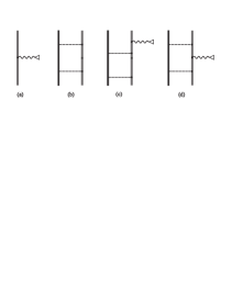
FIG. 1.: Diagrams representing the interaction of a bound electron with the external magnetic field (a), the lowest-order nuclear-polarization effect (b), and the nuclear-polarization correction to the bound-electron $g$ factor (c) and (d). The heavy line denotes the nucleus. The contribution corresponding to the graph (c) should be counted twice.

TABLE I.: Nuclear-polarization effects to the $g$ factor of K- and L-shell electrons in hydrogenlike ions. Column (a): contributions from low-lying rotational and vibrational nuclear modes using experimental values for nuclear excitation energies $\omega_{L}$ and electric transition strengths $B(EL)$; (b) contributions from giant resonances employing empirical sum rules [20,23]; (c) total effect. The numbers in parentheses are powers of ten.

	$-\Delta g_{1s}$				$-\Delta g_{2s}$				$-\Delta g_{2p_{1/2}}$
	(a)	(b)	(c)		(a)	(b)	(c)		(a)	(b)	(c)
${}^{\ 84}_{\ 36}$Kr	$1.0(-10)$	$1.1(-9)$	$1.2(-9)$		$1.3(-11)$	$1.5(-10)$	$1.6(-10)$		$1.5(-13)$	$1.8(-12)$	$2.0(-12)$
${}^{102}_{\ 44}$Ru	$1.2(-9)$	$3.3(-9)$	$4.5(-9)$		$1.7(-10)$	$4.5(-10)$	$6.2(-10)$		$3.1(-12)$	$8.6(-12)$	$1.2(-11)$
${}^{112}_{\ 48}$Cd	$1.4(-9)$	$5.5(-9)$	$6.9(-9)$		$1.9(-10)$	$7.7(-10)$	$9.6(-10)$		$4.3(-12)$	$1.8(-11)$	$2.2(-11)$
${}^{142}_{\ 60}$Nd	$1.7(-9)$	$2.1(-8)$	$2.3(-8)$		$2.6(-10)$	$3.2(-9)$	$3.5(-9)$		$9.8(-12)$	$1.2(-10)$	$1.3(-10)$
${}^{158}_{\ 64}$Gd	$4.7(-8)$	$3.4(-8)$	$8.1(-8)$		$7.3(-9)$	$5.1(-9)$	$1.2(-8)$		$3.1(-10)$	$2.3(-10)$	$5.4(-10)$
${}^{162}_{\ 66}$Dy	$6.0(-8)$	$4.1(-8)$	$1.0(-7)$		$9.3(-9)$	$6.3(-9)$	$1.6(-8)$		$4.3(-10)$	$3.0(-10)$	$7.3(-10)$
${}^{174}_{\ 70}$Yb	$8.6(-8)$	$6.2(-8)$	$1.5(-7)$		$1.4(-8)$	$9.8(-9)$	$2.4(-8)$		$7.4(-10)$	$5.4(-10)$	$1.3(-9)$
${}^{196}_{\ 78}$Pt	$4.5(-8)$	$1.3(-7)$	$1.8(-7)$		$7.6(-9)$	$2.2(-8)$	$3.0(-8)$		$5.5(-10)$	$1.6(-9)$	$2.2(-9)$
${}^{202}_{\ 80}$Hg	$2.1(-8)$	$1.6(-7)$	$1.8(-7)$		$3.7(-9)$	$2.8(-8)$	$3.2(-8)$		$2.9(-10)$	$2.1(-9)$	$2.4(-9)$
${}^{208}_{\ 82}$Pb	$2.2(-8)$	$2.0(-7)$	$2.2(-7)$		$3.8(-9)$	$3.4(-8)$	$3.8(-8)$		$3.2(-10)$	$2.9(-9)$	$3.2(-9)$
${}^{232}_{\ 90}$Th	$6.0(-7)$	$4.2(-7)$	$1.0(-6)$		$1.1(-7)$	$7.8(-8)$	$1.9(-7)$		$1.2(-8)$	$8.4(-9)$	$2.0(-8)$
${}^{238}_{\ 92}$U	$9.0(-7)$	$5.0(-7)$	$1.4(-6)$		$1.8(-7)$	$9.5(-8)$	$2.7(-7)$		$1.9(-8)$	$1.1(-8)$	$3.0(-8)$

REFERENCES

• [1] N.Β Hermanspahn, H.Β HΓ€ffner, H.-J.Β Kluge, W.Β Quint, S.Β Stahl, J.Β VerdΓΊ, and G.Β Werth, Phys. Rev. Lett. 84, 427 (2000).
• [2] H.Β HΓ€ffner, T.Β Beier, N.Β Hermanspahn, H.-J.Β Kluge, W.Β Quint, S.Β Stahl, J.Β VerdΓΊ, and G.Β Werth, Phys. Rev. Lett. 85, 5308 (2000).
• [3] T.Β Beier, H.Β HΓ€ffner, N.Β Hermanspahn, S.G.Β Karshenboim, H.-J.Β Kluge, W.Β Quint, S.Β Stahl, J.Β VerdΓΊ, and G.Β Werth, Phys. Rev. Lett. 88, 011603 (2002).
• [4] S.G.Β Karshenboim, in The Hydrogen Atom, edited by S.G.Β Karshenboim et al. (Springer, Berlin, 2001), p. 651; hep-ph/0008227.
• [5] G.Β Werth, H.Β HΓ€ffner, N.Β Hermanspahn, H.-J.Β Kluge, W.Β Quint, and J.Β VerdΓΊ, in The Hydrogen Atom, edited by S.G.Β Karshenboim et al. (Springer, Berlin, 2001), p. 202.
• [6] S.A.Β Blundell, K.T.Β Cheng, and J.Β Sapirstein, Phys. Rev. A 55, 1857 (1997).
• [7] H.Β Persson, S.Β Salomonson, P.Β Sunnergren, and I.Β Lindgren, Phys. Rev. A 56, R2499 (1997).
• [8] T.Β Beier, Phys. Rep. 339, 79 (2000).
• [9] A.Β Czarnecki, K.Β Melnikov, and A.Β Yelkhovsky, Phys. Rev. A 63, 012509 (2000).
• [10] V.M.Β Shabaev, Phys. Rev. A 64, 052104 (2001).
• [11] A.Β Yelkhovsky, hep-ph/0108091.
• [12] S.G.Β Karshenboim, V.G.Β Ivanov, and V.M.Β Shabaev, Zh. Γ‰ksp. Teor. Fiz. 120, 546 (2001)[Sov. Phys. JETP 93, 477 (2001)].
• [13] D.A.Β Glazov and V.M.Β Shabaev, Phys. Lett. A 297, 408 (2002).
• [14] V.M.Β Shabaev and V.A.Β Yerokhin, Phys. Rev. Lett. 88, 091801 (2002).
• [15] V.M.Β Shabaev, D.A. Glazov, M.B. Shabaeva, V.A. Yerokhin, G. Plunien and G. Soff, Phys. Rev. A (to be published).
• [16] S.A.Β Zapryagaev, Opt. Spektrosk. 47, 18 (1979)[Opt. Spectrosc. 47, 9 (1979)].
• [17] G.Β Plunien, B.Β MΓΌller, W.Β Greiner, and G.Β Soff, Phys. Rev. A 43, 5853 (1991).
• [18] A.Β Haga, Y.Β Horikawa, and Y.Β Tanaka, Phys. Rev. A 65, 052509 (2002).
• [19] G.Β Plunien and G.Β Soff, Phys. Rev. A 51, 1119 (1995); 53, 4614(E) (1996).
• [20] A.V.Β Nefiodov, L.N.Β Labzowsky, G.Β Plunien, and G.Β Soff, Phys. Lett. A 222, 227 (1996).
• [21] A.I.Β Akhiezer and V.B.Β Berestetskii, Quantum Electrodynamics (Interscience, New York, 1965).
• [22] V.M.Β Shabaev, J. Phys. B 24, 4479 (1991).
• [23] G.A.Β Rinker and J.Β Speth, Nucl. Phys. A 306, 397 (1978).
• [24] W.R.Β Johnson, S.A.Β Blundell, and J.Β Sapirstein, Phys. Rev. A 37, 307 (1988).
Refer to caption