Confidence Limits and their Robustness

Abstract

Confidence limits are common place in physics analysis. Great care must be taken in their calculation and use, especially in cases of limited statistics when often one-sided limits are quoted. In order to estimate the stability of the confidence levels to addition of more data and/or change of cuts, we argue that the variance of their sampling distributions be calculated in addition to the limit itself. The square root of the variance of their sampling distribution can be thought of as a statistical error on the limit. We thus introduce the concept of statistical errors of confidence limits and argue that not only should limits be calculated but also their errors in order to represent the results of the analysis to the fullest. We show that comparison of two different limits from two different experiments becomes easier when their errors are also quoted. Use of errors of confidence limits will lead to abatement of the debate on which method is best suited to calculate confidence limits.

I Introduction

Confidence limits are used to express the results of experiments that are not yet sensitive to discover the object of their searches. In such cases, often a one-sided limit is used to delimit the quantity of interest. Limits from different experiments are compared and attempts are made to combine them. These limits can fluctuate up or down with the addition of more data or the changing of the analysis parameters. A measure of the robustness of the limits is given by the width of the sampling distribution of these limits, where the sampling distribution is obtained over an ensemble of similar experiments simulated by Monte Carlo. The standard deviation of the sampling distribution of such limits can be thought of as an error on the limit.

We introduce the concept of error of confidence limits by a simple Gaussian example. Consider a sample of $n$ events, where $n=10$, characterised by the variable $x$ distributed as a unit Gaussian, with a mean value $\mu=0$ and standard deviation $\sigma=1$. Then the average value $\bar{x}$ of the $n$ events will be distributed as a Gaussian of mean value zero and standard error $\sigma$/$\sqrt{(}n)$. The unbiased estimate of $\sigma$, the variance of the distribution is given by $s$ where,

$$s^{2}=\frac{1}{n-1}\sum_{i=1}^{i=n}(x_{i}^{2}-\bar{x}^{2})$$ (1)

Figure 1 shows the distribution $\bar{x}$ of our sample of 10 events for a large number of samples. The expected value $\bar{x}$ is zero and its standard deviation is 0.32 which is consistent with the theoretical value of $\sigma/\sqrt{(}n)$=0.316.

Figure 1: The distribution of the sample average $\bar{x}$ over a large sample of events.

Figure 2 shows a histogram of $s$ deduced from a sample of 10 events for a large number of such samples. The average value of $s$ is $\approx$ 1.0, showing that $s$ is an unbiased estimator of $\sigma$. The important point to note is that $s$ also has a variance and that its standard deviation is $0.23$. This is as expected from theory where the error on the standard deviation of a Gaussian sample weather is $\approx\sigma/\sqrt{(}2n)$=0.223.

Figure 2: Unbiased estimate $s$ of the standard deviation of the $\sigma$ of the Gaussian distribution deduced from a sample of $n=10$ events. The average value of $s$ is $\approx$ 1.0 and its standard deviation is 0.23.

Having got the value of $\bar{x}$ and $s$ for our sample, one can proceed to work out confidence limits for our observation. The two-sided 68$\%$ CL limits for our observation of $\bar{x}$ will be given by the standard error $\sigma(\bar{x})$ of $\bar{x}$ and we would write the observation of $\bar{x}$ from our sample as

$$\bar{x}\pm\sigma(\bar{x})=\bar{x}\pm s/\sqrt{(}n)=-0.188\pm 0.408$$ (2)

where the numbers correspond to our sample of 10 events. Note that the standard error $\sigma(\bar{x})$ = 0.408 derived from our sample of 10 events is quite different from the theoretical value of 0.32, but this is merely due to statistical fluctuation.

One can also work out the two-sided 90% CL limits for our observation of $\bar{x}$ which would correspond to $\pm 1.64~{}\sigma(\bar{x})$ and quote the 90% CL limits as $-0.188\pm 0.669$, which is the value observed for our sample of 10 events.

Figure 3 shows the distribution of the 90% CL two-sided errors on the sample average, over a large number of samples. The mean value of the distribution is 0.505 which is close to the theoretical value of 1.64 $\sigma(\bar{x})$=0.519. Note that the standard deviation of the 90% CL errors in Figure 3 is 0.12. We can also calculate the standard deviation of the 90% CL error from our sample as 1.64 $\sigma(\bar{x})/\sqrt{(}2n)$ and this is plotted in figure 4. The mean value of the standard deviation of the 90% CL error in figure 4 is 0.113, in line with the theoretical value of 0.116.

Figure 3: The distribution of the calculated two-sided 90% CL errors of the mean value of the sample.

Figure 4: The distribution of the calculated error on the two-sided 90% CL error of the mean value of the sample.

When the mean value is of interest, we quote the mean value and the standard error on the mean value as in equation 2. This enables us to gauge the fluctuations in the mean value from sample to sample. When the confidence limit is of interest, we propose that we quote the confidence limit along with its standard error. This would enable us to gauge the significance and stability of the confidence level. In our example we would write this as

$$\bar{x}-1.64\sigma(\bar{x})\pm\sigma_{90}<\mu<\bar{x}+1.64\sigma(\bar{x})\pm\sigma_{90}~{}at~{}90\%~{}CL$$ (3)

where $\mu$ is the expectation value of $\bar{x}$ and the standard error $\sigma_{90}$ on the 90% CL limit would be given by

$$\sigma_{90}\approx\sigma(\bar{x})\sqrt{(1+(1.64)^{2}/(2n)}$$ (4)

In our sample of 10 events, this would lead to

$$-0.857\pm 0.434<\mu<0.481\pm 0.434~{}at~{}90\%~{}CL$$ (5)

Note that the error on the lower and upper 90% CL limits are correlated by the error on $\bar{x}$ which they have in common. Half the difference between the lower and uper 90 % CL limits is $1.64\sigma(\bar{x})$ and its error is 1.64$\sigma(\bar{x})/\sqrt{(}2n)$. These two errors added in quadrature yield the formula in equation 4. The error in the 90% CL limit indicates to the reader the stability of the limit and the statistical significance of the result.

Very often, we are not interested in the mean value of our observations but are more interested in the confidence limits, due to the low statistics of the observation. We may only be interested in an upper (one-sided) bound. So we would quote a 95% CL upper bound on $\mu$ as

$$\mu<0.481\pm 0.434~{}at~{}95\%~{}CL$$ (6)

A second sample of 10 events from the same distribution may yield a result

$$\mu<0.354\pm 0.335~{}at~{}95\%~{}CL$$ (7)

but we do not fall into the trap of declaring the second result a better limit than the first, because both the limits are the same within errors. If we did not quote the errors on the limits, we would be tempted to declare the second limit superior to the first.

Similarly, as analyses proceed in discovery searches, events can go in and out of samples, as cuts are refined and more data is accumulated. Appearance of a single event in a sample can change the confidence limit drastically, as was the case in the search for the top quark. These changes can be understood as fluctuations of the confidence limit within errors, if we were to quote not only the confidence limit but also its error.

II Reconciliation with the Neyman definition of Confidence limits

The construction of confidence levels as written down by Neyman neyman may be understood within the context of our current example as follows. Using our first sample of 10 events drawn from a unit Gaussian, we calculate a mean value $\bar{x}=-0.188$. Let us assume, for the sake of argument, that we know the variance of the mean value to be $1.0/\sqrt{(}10)$. In this case, we can construct the Neyman confidence level for $\mu$, the expectation value of $\bar{x}$, as illustrated in Fig. 5. The parameter $\mu$ is plotted on the ordinate and $\bar{x}$ is plotted on the abscissa. For each value of $\mu$, the 90% CL limits of $\bar{x}$ are delineated by horizontal lines that are delimited by the curves $\bar{x}_{1}(\mu)$ and $\bar{x}_{2}(\mu)$, assuming $\bar{x}$ is distributed about $\mu$ with variance $1.0/\sqrt{(}10)$. If the true value of $\mu$ is $\mu_{0}$, then $\bar{x}_{1}(\mu_{0})<\bar{x}<\bar{x}_{2}(\mu_{0})$ with 90% probability. If we now measure a value of $\bar{x}=-0.188$, then we can construct the interval AB which will contain the true value of $\mu_{0}$ if and only if $\bar{x}_{1}(\mu_{0})<\bar{x}<\bar{x}_{2}(\mu_{0})$. In other words the interval AB has a probability of 90% (also called “coverage”) of containing the true value $\mu_{0}$. The interval AB is thus defined to be the 90% CL interval of $\mu$.

If we were however to repeat our measurement of $\bar{x}$ by creating other samples of 10 events each, we would get different lines AB, each of which would have a 90% chance of containing the true value $\mu_{0}$. Most of the time, one is interested in a central value of $\bar{x}$ and an interval such as AB to denote the statistical errors (robustness) of the measurement of $\bar{x}$. However, in experiments with poor statistics, the central value $\bar{x}$ is often not of interest and the one-sided limit (either point A or B) is often quoted. At this stage, the points A or B become point measurements in their own right, and it is informative to quote their statistical errors in order to evaluate their robustness.

This is illustrated further in Fig. 6, where we now no longer assume we know the variance of $\bar{x}$. This is computed from the data and will fluctuate from sample to sample. These so-called “nuisance variables” are integrated over to yield a final confidence limit in usual practice, which would be appropriate if one were interested in the central value of $\bar{x}$. If however, one is interested in the one-sided limit B, it would be appropriate to use them to estimate the robustness of the point B due to statistical fluctuations. We use the error bands shown for $\bar{x}$ and $\sigma(\bar{x})$ in the figure to compute the sampling error band on the point B.

Figure 5: The Neyman construction of the confidence level for our example

Figure 6: The Neyman construction modified to illustrate fluctuations in $\bar{x}$ and $\sigma({\bar{x})}$ for our example. The error band due to $\sigma(\bar{x})$ and band due the error in $\sigma(\bar{x})$ are shown. These are added in quadrature to produce the sampling error band of point B.

III An Illustrative example

We can illustrate the need for confidence limits errors using the following example. In 1995, the DØ collaboration published limits on the top quark mass and cross section dzero . Figure 7 shows dzero the 95% CL upper limit on top quark production as a function of top quark mass using 13.5 pb^-1 of data. The confidence limit curve is used to derive a lower limit of 128 GeV/c² for the top quark mass at 95% CL. In the same paper, another figure, reproduced here as Figure  8 shows the top quark production cross section as a function of the top quark mass. This curve has a 1 $\sigma$ error band around it. But the top quark production cross section may be thought of as the 50% CL upper/lower bound on the cross section. Surely, if the 50% CL limit has an error band around it, the 95% CL limit should also have its own error band.

Figure 7: The 95% confidence level dzero on $\sigma_{t\bar{t}}$ as a function of top quark mass. Also shown are central (dotted line) and low (dashed line) theoretical cross section curves txsect .

Figure 8: Measured $t\bar{t}$ production cross section (solid line, shaded band = one standard deviation error) as a function of top mass dzero . Also shown are central (dotted line), high and low (dashed lines) theoretical cross section curves txsect .

In what follows, we show how to calculate errors in confidence levels in general and use the method to calculate the error in the 95% CL curve shown in Figure 7.

IV A general algorithm to calculate errors in Confidence Limits

Most experiments have elaborate algorithms to calculate confidence limits for their results. Such algorithms will include detailed calculations and parametrizations of efficiencies and acceptances. In addition, they will have several other input parameters such as the number of events observed, total integrated luminosity and the error on the luminosity. Let us denote the input parameters as $a_{i},~{}i=1,n$. The output of such a program will be the confidence limits $C_{\alpha},~{}\alpha=1,k$. Figure 9 illustrates this general case.

Figure 9: Schematic “black box” representation of a general confidence limit calculating algorithm, that has input parameters $a_{1},a_{2}..a_{4}$ and outputs a confidence level $C$ in a single variable.

Then, for small changes in the input parameters, the following equations hold.

$$\delta C_{\alpha}=\frac{\delta C_{\alpha}}{\delta a_{i}}\delta a_{i}$$ (8)

$$<\delta C_{\alpha}\delta C_{\beta}>=\frac{\delta C_{\alpha}}{\delta a_{i}}\frac{\delta C_{\beta}}{\delta a_{j}}<\delta a_{i}\delta a_{j}>$$ (9)

where the repeated indices $i,j$ are meant to be summed over and the symbols $<>$ indicates the average over the enclosed quantities. The quantity on the left hand side of the equation is the error matrix in the confidence limits $C_{\alpha}$, denoted $E_{CC}$. The above equation can be re-written in matrix form as

$$E_{CC}=\tilde{T}E_{aa}T$$ (10)

where $E_{aa}$ is the error matrix of the input parameters $a_{i},~{}i=1,n$ and $T$ is the transfer matrix, such that $T_{\alpha,i}=\frac{\delta C_{\alpha}}{\delta a_{i}}$. $T$ can be determined numerically by varying the input parameters to the limits algorithm. The error matrix $E_{aa}$ should be known to the experimenter, yielding the required error matrix $E_{CC}$.

IV.1 An Example

Let us consider the calculation of $C$, the 95% CL upper limit to the top quark cross section as published in reference dzero . The output of the limits algorithm is $C$. The input parameters can be taken as three, namely $a_{1}$, the total number of top quark events observed, $a_{2}$, the luminosity$\times$efficiency$\times$branching ratio of the channels under consideration, summed over the channels and $a_{3}$, the error in the luminosity. We have used a single parameter $a_{2}$ summed over the channels to simplify the calculation. In principle, all channels may be varied independently, but since they are uncorrelated, and the dominant error is due to the common luminosity factor, the above simplification will result. We use this example for illustrative purposes to show how such a calculation may proceed.

The error matrix of the parameters $E_{aa}$ is a 3$\times$3 diagonal matrix, since the parameters are uncorrelated. The variance of $a_{1}$ is the number of events observed, the variance of $a_{2}$ is calculated using the error in luminosity, and the variance of $a_{3}$ is calculated assuming that there is a 50% uncertainty in the error in the luminosity. The transfer matrix $T$ is calculated by numerical differentiation.

Figure 10 shows the contribution to $\sigma_{C}$, the error in the 95% CL upper limit to the cross section, due to the three parameters $a_{1}$, $a_{2}$ and $a_{3}$ as a function of the top quark mass. The overall error $\sigma_{C}$, obtained by adding the component errors in quadrature, is also shown as a function of the top quark mass. It can be seen that the contribution due to uncertainties in $a_{1}$, is negligible. So we are not sensitive to errors in our guess of 50% uncertainty to the error in the luminosity. The overall error is dominated by the fluctuation in the total number of events. This example thus graphically illustrates why confidence limits fluctuate up and down as events fall in and out of the selected sample as the analysis proceeds and more data is accumulated. The 95% CL upper limit to the cross section is merely fluctuating within its error as all statistical quantities do. When we are interested in a confidence limit, it thus behooves us to compute not only that limit but also its error.

Figure 10: The components of $\sigma_{C}$, the error in the 95% CL top quark cross section upper limit, due to uncertainties in (a) error in luminosity (b) Luminosity$\times$efficiency$\times$branching ratio (c) The overall number of events observed as a function of top quark mass. (d) shows the overall error $\sigma_{C}$.

We may superimpose these errors on Figure 7 yielding Figure 11. The 95% CL lower limit to the top quark mass can then be quoted as 128${}^{+14}_{-18}$ GeV/c², the error bars indicating the range of fluctuation for the mass limit. This implies that if one were to repeat the DØ experiment numerous times with an integrated luminosity of 13.5 pb^-1 fluctuating within its errors, one would expect to get a top quark lower mass limit that fluctuates within the errors quoted.

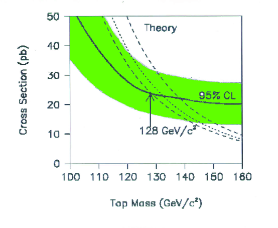
Figure 11: The DØ 95% CL upper limit to the top quark cross section dzero with its accompanying error band, as calculated by the method in the text.

V Combining limits

Combining limits from two different experiments is difficult at best. We remark here that in simple Gaussian cases, quoting the limit and its error provides us with enough information to make a combined result, as may be seen by examining equations 3 and 4. Using the value of the limit and its error, we may deduce $\bar{x}$ and $\sigma(\bar{x})$, if the number of events $n$ in the sample is known. Having the mean and its variance in each case, we can combine the Gaussians, leading to a new variance for the combined data. The combined mean of the two distributions can be found as usual by the weighted average of the two means, the weights being the inverse variances. It must be emphasized that the combined limit is not simply the weighted average of the two limits as in the case of the means.

One can further ask if the two limits are consistent with each other, if the errors on the limits are quoted, as shown below.

VI Comparing Limits from two different algorithms

When two different algorithms are used on the same data, two different limits will result that are correlated. The correlations will be due to the common input into the two algorithms. We can think of the “black box” in Fig. 9 as consisting of two different algorithms producing as output $C_{1}$ and $C_{2}$, the two confidence levels in question, using the same common input $a_{i},~{}i=1,n$. We can then use equation 10 to work out $E_{CC}$, the error matrix of the two confidence level algorithms and use this matrix to decide whether the two confidence levels are significantly different from each other as per,

$$var(C_{1}-C_{2})=var(C1)+var(C2)-2cov(C1,C2)=E_{11}+E{22}-2E_{12}$$ (11)

VII Conclusions

We have motivated the concept of statistical error for a confidence limit, as the standard deviation of the sampling distribution of such limits over an ensemble of similar experiments. In cases of limited statistics, our estimates of the confidence limits can fluctuate significantly. Comparing confidence limits becomes more meaningful when these errors are quoted. Different methods exist (e.g Bayesian, Frequentist) for calculating these limits. The differences between limits computed in the same experiment using different methods will lose their significance if the limits are shown to be the same within their sampling error. Often in analyses with limited statistics, the appearance of a new event can make significant differences to the limit calculation. An error analysis of the limit will show that the limit is exhibiting statistical fluctuation as it is entitled to. We propose that experimenters publish confidence limits to their data accompanied by the error on the limits.

VIII Acknowledgements

The author wishes to thank Roger Barlow, Bob Cousins, Louis Lyons, Harrison Prosper, Byron Roe, and Tom Trippe for helpful comments.

References

- (1) C.E. Weatherburn, “A first course in Mathematical Statistics”, Cambridge University press, Page 137.
- (2) J.Neyman, Phil. Trans. Royal Soc. London, Series A, 236, 333 (1937), reprinted in A Selection of Early Statistical Papers on J. Neyman (University of California Press, Berkeley, 1967).
- (3) “Top quark search with the DØ 1992-1993 data sample”, Phys.Rev.D52:4877(1995)
- (4) E.Laenen, J.Smith, W. van Neerven, Phys. Lett. 321B, 254 (1994); Nucl. Phys. B368, 543(1992).