Global Stationary Phase and the Sign Problem

Abstract

We present a computational strategy for reducing the sign problem in the evaluation of high dimensional integrals with non-positive definite weights. The method involves stochastic sampling with a positive semidefinite weight that is adaptively and optimally determined during the course of a simulation. The optimal criterion, which follows from a variational principle for analytic actions $S(z)$, is a global stationary phase condition that the average gradient of the phase $\mathrm{Im}S$ along the sampling path vanishes. Numerical results are presented from simulations of a model adapted from statistical field theories of classical fluids.

A familiar problem that arises in the context of lattice gauge theorylgt , quantum chemistryquantum1 , correlated electron physicsloh , and equilibrium field theories of classical fluidsghfrev , is the evaluation of integrals of the form

$$Z=\int_{C_{1}}dx\;\exp[-S(x)]$$ (1)

where the path of integration $C_{1}$ is the real axis and the action (or effective Hamiltonian) $S(x)$ is complex. In the cases of primary interest $x\in R^{n}$ is a n-vector representing a discrete representation (lattice sites or spectral elements) of one or more classical or quantum fields. The dimension $n$ is typically large, of order $10^{3}-10^{6}$. Here we shall use one-dimensional notation, although the formalism is primarily intended for cases of $n\gg 1$.

For real $S(x)$, there are a variety of powerful methods available for evaluating $Z$, including Monte Carlo and (real) Langevin simulationsbinder . However, in the case of complex $S=S_{R}+iS_{I}$, the integrand is not positive semidefinite, so the Monte Carlo method is not immediately applicable. Simulations can be carried out using the positive semidefinite weight $\exp(-S_{R})$, but then an oscillatory phase factor of $\exp(-iS_{I})$ must be included in the computation of averageslin . The rapid oscillations in this factor (the “sign problem”), which become more pronounced for large $n$, can dramatically slow convergence in such simulations. Alternatively, a “complex Langevin” simulation technique has been devised in which the field variables $x$ are extended to the complex plane and a Langevin trajectory prescribed for the purpose of generating Markov chains of statesparisi . Unfortunately this method is not guaranteed to converge and pathological behavior has been noted for specific modelslee ; schoenmaker . In the present letter we describe a new simulation approach that is useful for reducing the sign problem in integrals of the form of Eq. (1), where $S(z)$ is an analytic function of the complex n-vector $z=x+iy$.

We begin by considering a displacement of the original integration path along the real $x$ axis, $C_{1}$ to a new parallel path $C_{y}$ defined by $z=x+iy,\;x_{j}\in(-\infty,\infty)$, in which $y\in R^{n}$ is an arbitrary displacement of $C_{1}$ along the imaginary axis. Note that the displacement $y_{j}$ need not be uniform in $j$ for the $n>1$ case. Provided $S(z)$ is analytic in the rectangular strip bounded by $C_{1}$ and $C_{y}$ and $|\exp[-S(R+iy)]|\rightarrow 0$ for $R\rightarrow\pm\infty$, it follows that

$$Z=\int_{C_{y}}dz\;\exp[-S(z)]=\int_{C_{y}}dx\;\exp[-S(x+iy)]$$ (2)

and the resulting $Z$ is independent of the choice of $y$. Upon decomposing $S$ into real and imaginary parts $S_{R}(x,y)+iS_{I}(x,y)$, $Z$ can be rewritten as

$$Z=Z_{y}\int_{C_{y}}dx\;P_{y}(x)\exp[-iS_{I}(x,y)]$$ (3)

where $Z_{y}\equiv\int_{C_{y}}dx\;\exp[-S_{R}(x,y)]$ and $P_{y}(x)$ is a normalized, positive semidefinite, probability distribution for a random variable $x$ at the fixed value of $y$:

$$P_{y}(x)=\exp[-S_{R}(x,y)]/Z_{y}$$ (4)

It follows that the average of an analytic observable $f(x)$ can be evaluated alternatively from the formulas

$$\langle f(x)\rangle = Z^{-1}\int_{C_{1}}dx\;\exp[-S(x)]f(x)$$ (5)

$$= \frac{\langle\exp[-iS_{I}(x,y)]f(x+iy)\rangle_{y}}{\langle\exp[-iS_{I}(x,y)]\rangle_{y}}$$

where $\langle h(x)\rangle_{y}\equiv\int_{C_{y}}dx\;P_{y}(x)h(x)$ denotes an average with probability weight $P_{y}(x)$.

It is the second expression in Eq. (5) that is of interest in the present letter. A poor choice of $y$ will lead to significant oscillations in the phase factor $\exp[-iS_{I}(x,y)]$ as $x$ is stochastically varied along the sampling path $C_{y}$ in a simulation. This would drive both numerator and denominator in Eq. (5) to zero and dramatically slow or prevent convergence of average quantities of interest. One approach to alleviate this difficulty would be to choose $y=y^{*}$, where $y^{*}$ is the imaginary component of a saddle point $z^{*}$ defined by $S^{\prime}(z^{*})=0$. The deformed integration path $C_{y^{*}}$ would then be a line passing through the saddle point parallel to the real axis. If this path happened to be a constant phase (steepest ascent) path locally around the saddle point, then the phase oscillations would be reduced on trajectories that remain close to the saddle pointbender . In general, however, path $C_{y^{*}}$ will not be a a constant phase path, even in the close vicinity of $z^{*}$. A local analysis about each saddle point, costing $O(n^{2})$ in computational effort, can be used to identify proper constant phase paths. However, in typical problems where field fluctuations are strong, significant weight is given to trajectories that are not localized around saddle points.

The essence of our method is a global strategy for selecting an optimal displacement $y$, denoted $\bar{y}$. To this end, we introduce a “generating” function (functional)

$$G(y)=\ln\int_{C_{y}}dx\;\exp[-S_{R}(x,y)]$$ (6)

Invoking the Cauchy-Riemann (CR) equations, it is straightforward to show that the first derivative of $G(y)$ is given by

$$\frac{\partial G(y)}{\partial y_{j}}=\langle\frac{\partial}{\partial x_{j}}S_{I}(x,y)\rangle_{y}$$ (7)

The second derivative follows from repeated application of the CR equations and an integration by parts

$$\frac{\partial^{2}G(y)}{\partial y_{j}\partial y_{k}} = \langle[\frac{\partial}{\partial x_{j}}S_{I}-\langle\frac{\partial}{\partial x_{j}}S_{I}\rangle_{y}][\frac{\partial}{\partial x_{k}}S_{I}-\langle\frac{\partial}{\partial x_{k}}S_{I}\rangle_{y}]\rangle_{y}$$ (8)

$$+ \langle[\frac{\partial}{\partial x_{j}}S_{R}][\frac{\partial}{\partial x_{k}}S_{R}]\rangle_{y},$$

which is the sum of two positive definite forms. It follows that $G(y)$ is manifestly a convex function for any $y$.

We now claim that the “optimal” choice $y=\bar{y}$ is such that

$$\frac{\partial G(y)}{\partial y_{j}}|_{\bar{y}}=\langle\frac{\partial}{\partial x_{j}}S_{I}(x,\bar{y})\rangle_{\bar{y}}=0$$ (9)

Evidently such a point would be a local minimum of $G(y)$. Moreover, it implies that $S_{I}$ has vanishing gradients on average along the sampling path $C_{\bar{y}}$. This condition can be viewed as a global, rather than localbender , stationary phase criterion and would seem to be an excellent way to minimize the effect of phase fluctuations. Since $G(y)$ has a unique minimum, it follows that $\bar{y}_{j}$ is homogeneous in $j$ for bulk systems with translationally invariant actions. The method evidently produces nontrivial inhomogeneous $\bar{y}$ when applied to field theories in bounded geometries.

It remains to discuss how to incorporate this optimal choice of sampling path into a simulation algorithm. We propose the following “optimal path sampling” (OPS) algorithm:

1. Initialize vectors $x$ and $y=y^{k}$ with $k=0$.

2. Carry out a stochastic simulation in $x$ at fixed $y^{k}$ to generate a Markov chain of $x$ states of length $M$. $P_{y^{k}}(x)$ should be used as a statistical weight for importance sampling. The simulation method could be Metropolis Monte Carlo, its “smart” or “hybrid” variantskennedy , or a real Langevin technique.

3. Evaluate $G(y^{k})$ and $\partial G(y^{k})/\partial y^{k}$ by averaging over the $x$ configurations accumulated in the $M$-state simulation. Update $y$ to approach $\bar{y}$ by making a steepest descent step

   $$y^{k+1}=y^{k}-\lambda\frac{\partial G(y^{k})}{\partial y^{k}}$$

   where $\lambda$ is an adjustable relaxation parameter. Alternatively, the accumulated information on $G(y)$ could be used to carry out approximate line minimizations, which would permit conjugate gradient updates from $y^{k}$ to $y^{k+1}$.

4. Repeat steps 2 and 3 for $k=1,2,...$ until the sequence of $y^{k}$ converges to within some prescribed tolerance to $\bar{y}$. The simulation has now equilibrated.

5. Carry out a long stochastic simulation (“production run”) with statistical weight $P_{\bar{y}}(x)$.

6. Compute averages over the simulated states according to Eq. (5) with $y=\bar{y}$.

Evidently, the parameters $M$ and $\lambda$ can be adjusted to accelerate the “equilibration” period.

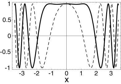
Figure 1: Variation of the phase factor of the Airy integrand $\mathrm{Re}[\exp(-iS_{I}(x,y,1))]$ with $x$ for $y=0$ (dashed) and $y=\bar{y}=1.19149$ (solid).

Our OPS method has some similarities to (and was inspired by) the complex Langevin (CL) simulation technique. In that approach, one generates a Markov chain of states in the complex plane by integrating the Langevin equationsparisi

$$\frac{\partial x}{\partial t}=-\mathrm{Re}\frac{dS}{dz}+\eta(t)$$ (10)

$$\frac{\partial y}{\partial t}=-\mathrm{Im}\frac{dS}{dz}$$ (11)

where $\eta(t)$ is a real Gaussian white noise with $\langle\eta(t)\rangle=0$ and $\langle\eta_{j}(t)\eta_{k}(t^{\prime})\rangle=2\delta(t-t^{\prime})\delta_{jk}$. Ensemble averages $\langle f(x)\rangle$ are computed as time averages of $f(x+iy)$ over the chain of states. Under conditions where the CL method converges, we have observed that $y$ drifts to a nearly constant value that is not associated with any saddle point $y^{*}$. Eq. (11) reduces approximately in this case to $\langle\mathrm{Im}\;dS/dz\rangle_{y}=0$, which is equivalent to the condition (9). The OPS technique is also distinct from so-called “stationary phase Monte Carlo” methods, which apply filtering and sparse sampling methods to suppress phase oscillationsquantum1 ; sabo . These methods are effective but apparently have no variational basis.

Before providing a numerical example of the OPS method, it is illustrative to see how our global stationary phase criterion works in a simple one dimensional example

$$\mathrm{Ai}(t)=\frac{1}{2\pi}\int_{-\infty}^{\infty}dx\;\exp[i(x^{3}/3+tx)],$$ (12)

which is a representation of the Airy function. In this case $S(x,t)=-i(x^{3}/3+tx)$ and Eq. (9) leads to $\bar{y}^{2}-\langle x^{2}\rangle_{\bar{y}}-t=0$. This equation has a single root, corresponding to the minimum of $G(y)$, that yields $\bar{y}(t)$. For example, $\bar{y}(1)=1.19149$. Of particular interest is the effect of the optimal displacement on phase oscillations. In Fig. 1 we plot $\mathrm{Re}[\exp(-iS_{I}(x,y,t))]$ verses $x$ at $t=1$ for $y=0$ (no shift) and $y=\bar{y}$ (optimal). Clearly the optimal shift dramatically suppresses phase oscillations over the interval $-2\lesssim x\lesssim 2$. The global stationary phase criterion has no effect outside this interval, because $P_{\bar{y}}(x)$ decays supra-exponentially there as $\sim\exp(-x^{2}\bar{y})$ and so no statistical weight is given to $|x|\gtrsim 2$.

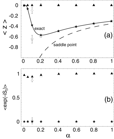
Figure 2: Comparison between OPS and CL simulations. (a): The average of $z=x+iy$ as a function of the parameter $\alpha$ for the model of Eq. (13) with $n=1$ and $\chi=1$. Open and filled symbols are results, respectively, from CL and OPS. Stars denote the average of the imaginary part $y$ and triangles the average of the real part $x$. The full line is the exact solution, the dashed line the corresponding saddle point. (b): The average sign $\exp(-iS_{I})$ for the same parameters as in (a). The convention for the symbols is the same as in (a). Error bars are comparable to the symbol sizes if not explicitly shown.

As a numerical test of the OPS method, we have carried out simulations of the model

$$S(x)=\sum_{j=1}^{n}[\alpha x_{j}^{2}+(x_{j+1}-x_{j})^{2}-\chi\exp(-ix_{j})]$$ (13)

which can be viewed as a lattice field theory for the one-dimensional classical Yukawa fluid in the grand canonical ensemble ($\alpha$ is a measure of interaction strength and $\chi$ is the activity). For the case of $n>1$, periodic boundary conditions are applied. The model has a saddle point $z_{j}^{*}=iy^{*}_{j}$ that lies on the imaginary axis and is homogeneous in the index $j$ (as well as an inhomogeneous “1d crystal-like” saddle point). Its location is given by the solution of $\chi\exp(y^{*}_{j})+2\alpha y^{*}_{j}=0$. The optimal displaced path $\bar{y}_{j}$ is homogeneous in $j$ and is given by the solution of $\chi\exp(\bar{y}_{j})\langle\cos x_{j}\rangle_{\bar{y}}+2\alpha\bar{y}_{j}=0$. We see that $y^{*}$ and $\bar{y}$ are coincident under conditions ($\alpha\gg 1$) where the random variable $x$ fluctuates closely about the saddle point $x^{*}=0$. In the strongly fluctuating regime ($\alpha\ll 1$), $\langle\cos x_{j}\rangle_{\bar{y}}$ will be dramatically reduced, resulting in a large shift of $\bar{y}$ away from $y^{*}$. These expectations are borne out in numerical simulations of the model.

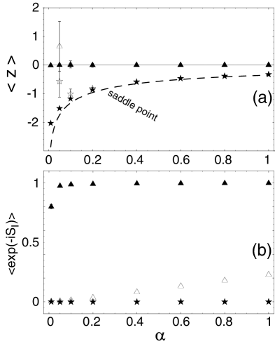
Figure 3: Comparison OPS and conventional MC. (a): The average of $z=x+iy$ as a function of the parameter $\alpha$ for the model of Eq. (13) with $n=10$ and $\chi=1$. Open and filled symbols are results, respectively, from MC and OPS. Stars, triangles, and dashed curve as in Fig. 2. (b): The average sign $\exp(-iS_{I})$ for the same parameters as in (a). At small $\alpha$ the real part of the sign in MC rapidly approaches zero, and the averages fail to converge. Error bars are comparable to the symbol sizes if not explicitly shown.

We have carried out conventional Metropolis Monte Carlo (MC)[i.e. Eq. (5) with $y=0$], OPS, and CL simulations of the model with action Eq. (13). The results were obtained from runs with a total of $10^{7}$ MC cycles or Langevin steps, a time step of 0.001 in the case of CL, and parameters $M=1000$, $\lambda=0.05$ for OPS. In Fig. 2 we compare the results obtained from OPS and CL simulations with $n=1$ and $\chi=1$. The top panel (a) shows $\langle z\rangle$ as a function of $\alpha$, while the bottom panel (b) displays the real and imaginary parts of the “sign” $\langle\exp(-iS_{I})\rangle$. In contrast to OPS, CL fails to converge, or converges very slowly, for $\alpha\lesssim 0.15$. Conventional MC also converges, but the average sign is approximately 0.8, as opposed to $\sim 1$ shown by the OPS.

It is often observedloh that the sign in conventional MC simulations decreases exponentially with $n$, causing a breakdown of the method. This is illustrated for the present model in Fig. 3 with parameters $n=10$ and $\chi=1$. The conventional MC method fails to converge for $\alpha\lesssim 0.1$ in contrast to OPS. Moreover, the real part of the sign is strongly suppressed in the MC results, even at large values of $\alpha$. The sign problem is evidently strongly suppressed, if not eliminated entirely for this model in OPS.

The OPS method is applicable to any field theory with an action $S(z)$ that is analytic throughout a domain of $z$ relevant to numerical simulations. This includes the important cases of classical fluids in the grand canonical ensemble and path integral formulations of time-dependent quantum chemical problems. Other situations including fluids in the canonical ensemble, strongly correlated electrons, and lattice gauge theories are characterized by analytic $\exp(-S)$, but with zeros along the real axis and hence logarithmic singularities in $S$. We believe that OPS will also be useful in such problems, however precautions should be taken to avoid crossing branch cuts in the steepest descent approach to the optimal displacement $\bar{y}$. Finally, we note that the displaced paths considered here were parallel to the real axis. Generalization of the method to optimize both the displacement and shape of the path could prove even more powerful.

In summary, we have identified a variational principle that permits a global stationary phase analysis of integrals of arbitrary dimension with analytic integrands. We expect that this technique will have important implications for analytical and numerical investigations of field theories in the complex plane.

- (1) I. Montvay and G. Münster, Quantum Fields on the Lattice (Cambridge University Press, Cambridge, 1994).
- (2) V. S. Filinov, Nuclear Physics B 271, 717 (1986); J. D. Doll and D. L. Freedman, Adv. Chem. Phys. 73, 289 (1988); N. Makri and W. H. Miller, Chem. Phys. Lett. 139, 10 (1987).
- (3) E. Y. Loh Jr. et al., Physical Review B 41, 9301 (1990).
- (4) G. H. Fredrickson, V. Ganesan, and F. Drolet, Macromolecules 35, 16 (2002); S. A. Baeurle, Phys. Rev. Lett. 89, 080602 (2002).
- (5) D. P. Landau and K. Binder, A Guide to Monte Carlo Simulations in Statistical Physics (Cambridge University Press, New York, 2000).
- (6) H. Q. Lin and J. E. Hirsch, Phys. Rev. B 34, 1964 (1986).
- (7) G. Parisi, Phys. Lett. B 131, 393 (1983); J. R. Klauder, Phys. Rev. A 29, 2036 (1984).
- (8) S. Lee, Nuclear Physics B 413, 827 (1994).
- (9) W. J. Schoenmaker, Physical Review D 36, 1859 (1987).
- (10) C. M. Bender and S. A. Orszag, Advanced Mathematical Methods for Scientists and Engineers (McGraw-Hill Publishing Company, New York, 1978).
- (11) A. D. Kennedy, Parallel Computing 25, 1311 (1999); P. J. Rossky and J. D. Doll, J. Chemical Physics 69, 4628 (1978).
- (12) D. Sabo, J. D. Doll, and D. L. Freedman, J. Chemical Physics 116, 3509 (2002).