The probability of making a correct decision in hypotheses testing as estimator of quality of planned experiments

S.I. Bityukov, N.V. Krasnikov

Abstract

In the report the approach to estimation of quality of planned experiments is considered. This approach is based on the analysis of uncertainty, which will take place under the future hypotheses testing about the existence of a new phenomenon in Nature. The probability of making a correct decision in hypotheses testing is proposed as estimator of quality of planned experiments. This estimator allows to take into account systematics and statistical uncertainties in determination of signal and background rates.

I Introduction

One of the common goals in the forthcoming experiments is the search for new phenomena. In estimation of the discovery potential of the planned experiments the background cross section (for example, the Standard Model cross section) is calculated and, for the given integrated luminosity $L$, the average number of background events is $n_{b}=\sigma_{b}\cdot L$. Suppose the existence of new physics leads to additional nonzero signal cross section $\sigma_{s}$ with the same signature as for the background cross section that results in the prediction of the additional average number of signal events $n_{s}=\sigma_{s}\cdot L$ for the integrated luminosity $L$. The total average number of the events is $<n>=n_{s}+n_{b}=(\sigma_{s}+\sigma_{b})\cdot L$. So, as a result of new physics existence, we expect an excess of the average number of events. Let us suppose the probability of the realization of $n$ events in the experiment is described by function $f(n;\lambda)$ with parameter $\lambda$.

In the report the approach to estimation of quality of planned experiments is considered. This approach is based on the analysis of uncertainty, which will take place under the future hypotheses testing about the existence of a new phenomenon in Nature.

We consider a statistical hypothesis

$H_{0}$: new physics is present in Nature

against an alternative hypothesis

$H_{1}$: new physics is absent in Nature.

The value of uncertainty is defined by the values of the probability to reject the hypothesis $H_{0}$ when it is true (Type I error)

$\alpha$ = $P(reject~{}H_{0}|H_{0}~{}is~{}true)$

and the probability to accept the hypothesis $H_{0}$ when the hypothesis $H_{1}$ is true (Type II error)

$\beta$ = $P(accept~{}H_{0}|H_{0}~{}is~{}false)$.

Here $\alpha$ is a significance of the test and $1-\beta$ is a power of the test.

We propose to use as estimator of the quality of planned experiments the probability of making a correct decision in the future hypotheses testing $1-\hat{\kappa}$

$$1-\hat{\kappa}=1-\frac{\hat{\alpha}+\hat{\beta}}{2},$$ (1)

and as estimator of the distinguishability of the hypotheses $1-\tilde{\kappa}$

$$1-\tilde{\kappa}=1-\frac{\hat{\alpha}+\hat{\beta}}{2-(\hat{\alpha}+\hat{\beta})},$$ (2)

where $\hat{\alpha}$ and $\hat{\beta}$ are the estimators of Type I error $\alpha$ and Type II error $\beta$ calculated by the applying of the equal-tailed test ($\hat{\alpha}=\hat{\beta}$).

The $1-\hat{\kappa}$ is the estimator of quality of planned experiments. This estimator allows to take into account systematics and statistical uncertainties b2 in determination of signal and background rates. The $1-\hat{\kappa}$ have no dependence on the choice what is $H_{0}$, what is $H_{1}$. This value is free from restrictions of such type. It is an advantage of our approach. We also propose to use an equal probability test b1 as a good approximation of the equal-tailed test for estimation of the probabilities $\hat{\alpha}$ and $\hat{\beta}$ in the case of Poisson distributions.

II What is meant by the probability of making a correct decision in hypotheses testing?

Suppose that the probability of the realization of $n$ events in experiment is described by the function $f(n;\lambda)$ with parameter $\lambda$ and we know the expected number of signal events $n_{s}$ and expected number of background events $n_{b}$.

Let us determine what we mean by the probability of making a correct decision under the future hypotheses testing about the presence or absence of the new phenomenon in Nature in case of carrying out the planned experiment. Let us use the frequentist approach, i.e. consider all the possible results of the experiment in cases when both the hypothesis $H_{0}$ is true or the hypothesis $H_{1}$ is true, define the criterion for the hypothesis choice and calculate the probability of making a correct decision. It is possible, because we construct the critical area in such a way that the probability of incorrect and, correspondingly, correct choice in favour of one of the hypothesis have no dependence on whether true is $H_{0}$ or $H_{1}$. So, we will consider 2 conditional distributions of probabilities (see, Fig.1)

$$\cases{f_{0}(n)=f(n;n_{s}+n_{b}),\cr f_{1}(n)=f(n;n_{b})}$$ (3)

making numerical calculations. We suppose that any prior suppositions about $H_{0}$ and $H_{1}$ can be included to $f_{0}(n)$ and $f_{1}(n)$.

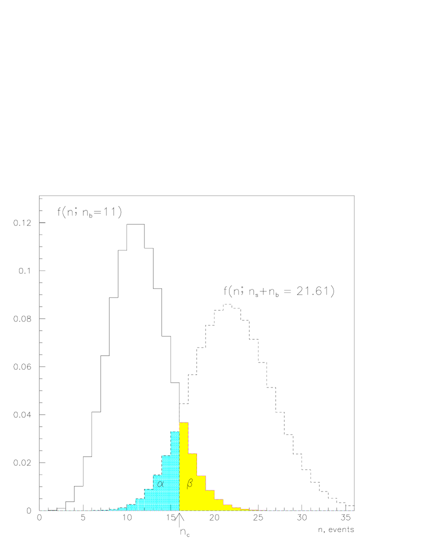
Figure 1: Equal probability test for the case $n_{b}=11$ and $n_{s}=10.61$ gives the critical value $n_{c}=16$ and, correspondingly, the probability of uncorrect decision $\hat{\kappa}=0.09$ and the measure of distinquishability of hypotheses $\tilde{\kappa}=0.1$.

After choosing a critical value (or a critical area) same way, it is possible to count up the estimators of Type I error $(\hat{\alpha})$ and Type II error $(\hat{\beta})$.

In the case of applying the equal-tailed test their combination

$$\hat{\kappa}=\frac{\hat{\alpha}+\hat{\beta}}{2}$$ (4)

is the probability of making incorrect choice in favour of one of the hypothesis.

The explanation is very simple. In actuality we must estimate the random value $\kappa=\alpha+\beta=\hat{\kappa}+e$, where $\hat{\kappa}$ is a constant term and $e$ is a stochastic term. The $\alpha$ is a fraction of incorrect decisions if the hypothesis $H_{0}$ takes place. In this case the $\beta$ is absent because the hypothesis $H_{1}$ is not realised in Nature. Correspondingly, the $\beta$ is a fraction of incorrect decisions if the hypothesis $H_{1}$ takes place. In this case the $\alpha$ is absent. Let us the hypothesis $H_{0}$ be true then the Type I error equals $\hat{\alpha}$ and the error of our estimator (Eq.4) is $\hat{e}=\hat{\kappa}-\hat{\alpha}=\displaystyle\frac{\hat{\alpha}+\hat{\beta}}{2}-\hat{\alpha}=-\frac{\hat{\alpha}-\hat{\beta}}{2}$. If hypothesis $H_{1}$ is true then the Type II error equals $\hat{\beta}$ and the error of the estimator is $\hat{e}=\hat{\kappa}-\hat{\beta}=\displaystyle\frac{\hat{\alpha}+\hat{\beta}}{2}-\hat{\beta}=\frac{\hat{\alpha}-\hat{\beta}}{2}$. By this mean the stochastic term takes the values $\displaystyle\pm\frac{\hat{\alpha}-\hat{\beta}}{2}$ and if we require $\hat{\alpha}=\hat{\beta}$ then both errors of the estimation are equal to 0    ($\hat{\kappa}-\hat{\alpha}=\hat{\kappa}-\hat{\beta}=0$). As a result the estimator (Eq.4) gives the probability of making an incorrect decision in future hypotheses testing. Really, if $\hat{\alpha}=\hat{\beta}$ and the $H_{0}$ takes place in Nature then $\hat{\kappa}=(\hat{\alpha}+\hat{\beta})/2=2\cdot\hat{\alpha}/2=\alpha$. In the same manner $\hat{\kappa}=\beta$ if the $H_{1}$ takes place. Accordingly, $\displaystyle 1-\hat{\kappa}$ is the probability to make a correct choice under the given critical value.

Under the hypotheses testing we can also estimate the measure $1-\tilde{\kappa}$ of distinguishability of the hypotheses $H_{0}$ and $H_{1}$  by the calculation of

$$\tilde{\kappa}=\frac{\hat{\alpha}+\hat{\beta}}{2-(\hat{\alpha}+\hat{\beta})}.$$ (5)

There are 3 possibilities.

• Distributions $f_{0}(n)$ and $f_{1}(n)$ have no overlapping, hence, the distributions are completely distinguishable and any result of the experiment will give the correct choice between hypotheses, i.e. $\tilde{\kappa}=0$.

• Distributions $f_{0}(n)$ and $f_{1}(n)$ coincide completely. It means, that it is impossible to get a correct answer, i.e. $f_{0}(n)$ and $f_{1}(n)$ are not distinguishable, i.e. $\tilde{\kappa}=1$.

• Distributions $f_{0}(n)$ and $f_{1}(n)$ do not coincide, but they have an overlapping, i.e. $\tilde{\kappa}$ is ratio of the probability of making incorrect choice to probability making correct choice in favour of one of the hypothesis.

III The choice of critical area

Let the probability of the realization of $n$ events in the experiment be described by Poisson distribution with parameter $\lambda$, i.e.

$$f(n;\lambda)=\frac{{\lambda}^{n}}{n!}e^{-\lambda}.$$ (6)

In this case the estimators of Type I and II errors, which will take place in testing of hypothesis $H_{0}$ versus hypothesis $H_{1}$, can be written as follows:

$$\cases{\displaystyle\hat{\alpha}=\sum^{n_{c}}_{i=0}{f(i;n_{s}+n_{b})}=\sum^{n_{c}}_{i=0}{f_{0}(i)},\cr\displaystyle\hat{\beta}=1-\sum^{n_{c}}_{i=0}{f(i;n_{b})}=1-\sum^{n_{c}}_{i=0}{f_{1}(i)},}$$ (7)

where $n_{c}$ is a critical value. Correspondingly, the magnitude $\displaystyle\hat{\kappa}=\frac{\hat{\alpha}+\hat{\beta}}{2}$ will have minimal value under applying of the equal probability test b1 with critical value (see, Fig.1)

$$n_{c}=\displaystyle[\frac{n_{s}}{ln(n_{s}+n_{b})-ln(n_{b})}],$$ (8)

where square brackets mean the integer part of a number. It is easy to show that the $\hat{\kappa}$ has a minimum if we require $f_{0}(i)=f_{1}(i)$ (for discrete distributions it corresponds to condition $f_{0}(i)\leq f_{1}(i)$), i.e.

$$\frac{n_{b}^{n_{c}}e^{-n_{b}}}{n_{c}!}=\displaystyle\frac{(n_{s}+n_{b})^{n_{c}}e^{-(n_{s}+n_{b})}}{n_{c}!}.$$ (9)

It is direct consequence of the equation

$$\hat{\kappa}=\frac{\hat{\alpha}+\hat{\beta}}{2}=\frac{1}{2}(1-\sum^{n_{c}}_{i=0}{(f_{1}(i)-f_{0}(i))}).$$ (10)

The value of $\hat{\kappa}$ decreases with increasing of $i$ from $0$ up to $i=n_{c}$. As soon as $f_{0}(i)>f_{1}(i)$ the value of $\hat{\kappa}$ increases.

Note that the equal probability test gives the results close to the results of the equal-tailed test in the case of Poisson distributions and we use it hereafter.

Following the given discourse, we can choose critical values so that $\hat{\kappa}$ could be minimal and the probability of correct decision $\displaystyle 1-\hat{\kappa}$ - maximum for any pair of distributions. As a result it is possible to say, that the value $\displaystyle 1-\hat{\kappa}$ under the optimum choice of critical value characterises the quality of planned experiment.

Notice, that such approach works for arbitrary distributions (see, Fig.2), including multidimentional ones.

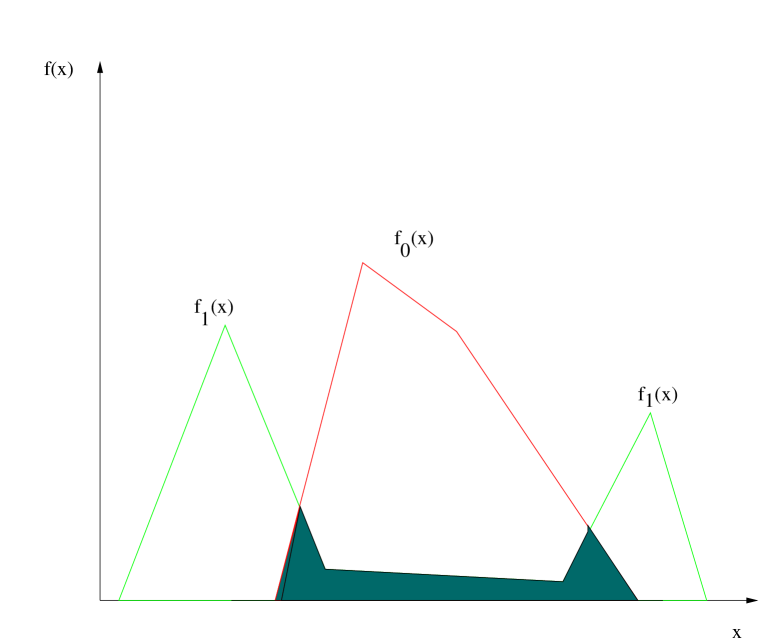
Figure 2: The estimation of uncertainty in hypotheses testing for arbitrary distributions.

IV How to take into account the statistical uncertainty in the determination of $n_{s}$ and $n_{b}$?

Let the values $n_{s}=\hat{n}_{s}$ and $n_{b}=\hat{n}_{b}$ be known from Monte Carlo calculations. In this case they are random variables. These values can be considered as estimators of unknown parameters. Consequently, the values $n_{c}$, $\alpha$ and $\beta$ are also random variables. It means that $1-\hat{\kappa}$ is the estimator of the probability of making a correct decision in hypotheses testing. Let us consider how the uncertainties in the knowledge of $n_{s}$ and $n_{b}$ influence the value of magnitude of the Probability of Making a Correct Decision in hypotheses testing (PMCD) $1-\hat{\kappa}$. Suppose, as before, that the streams of signal and background events are Poisson’s.

Let us write down the density of Gamma distribution $\Gamma_{a,n+1}$ as 

$$g_{n}(a,\lambda)=\displaystyle\frac{a^{n+1}}{\Gamma(n+1)}e^{-a\lambda}\lambda^{n},$$ (11)

where $a$ is a scale parameter, $n+1>0$ is a shape parameter, $\lambda>0$ is a random variable, and $\Gamma(n+1)=n~{}!$ is a Gamma function.

Let us set $a=1$, then for each $n$ a continuous function

$$g_{n}(\lambda)=\displaystyle\frac{\lambda^{n}}{n!}e^{-\lambda},~{}\lambda>0,~{}n>-1$$ (12)

is the density of Gamma distribution $\Gamma_{1,n+1}$ with the scale parameter $a=1$ (see Fig.3). The mean, mode, and variance of this distribution are given by $n+1,~{}n$, and $n+1$, respectively.

As it follows from the article Jaynes (see, also Frodesen ) and is clearly seen from the identity b4 (Fig.4)

$$\sum_{n=\hat{n}+1}^{\infty}{f(n;\lambda_{1})}+\int_{\lambda_{1}}^{\lambda_{2}}{g_{\hat{n}}(\lambda)d\lambda}+\sum_{n=0}^{\hat{n}}{f(n;\lambda_{2})}=1~{},~{}~{}~{}i.e.$$ (13)

$\displaystyle\sum_{n=\hat{n}+1}^{\infty}{\frac{\lambda_{1}^{n}e^{-\lambda_{1}}}{n!}}+\int_{\lambda_{1}}^{\lambda_{2}}{\frac{\lambda^{\hat{n}}e^{-\lambda}}{\hat{n}!}d\lambda}+\sum_{n=0}^{\hat{n}}{\frac{\lambda_{2}^{n}e^{-\lambda_{2}}}{n!}}=1~{}$

for any $\lambda_{1}\geq 0$ and $\lambda_{2}\geq 0$, the probability of true value of parameter of Poisson distribution to be equal to the value of $\lambda$ in the case of one observation $\hat{n}$ has probability density of Gamma distribution $\Gamma_{1,1+\hat{n}}$. The Eq.(13) shows that we can mix Bayesian and frequentist probabilities in the given approach. This identity does not leave a place for any prior except uniform. The bounds $\lambda_{1}$ and $\lambda_{2}$ fix it.

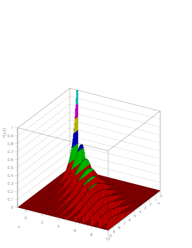
Figure 3: The behaviour of the probability density of the true value of parameter $\lambda$ for the Poisson distribution in case of $n$ observed events versus $\lambda$ and $n$. Here $f(n;\lambda)=g_{n}(\lambda)=\displaystyle\frac{\lambda^{n}}{n!}e^{-\lambda}$ is both the Poisson distribution with the parameter $\lambda$ along the axis $n$ and the Gamma distribution with a shape parameter $n+1$ and a scale parameter 1 along the axis $\lambda$.

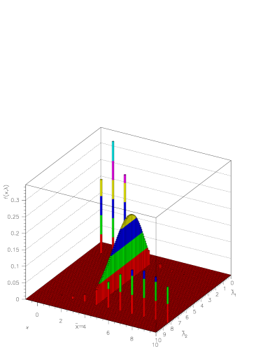
Figure 4: The Poisson distributions $f(n,\lambda)$ for $\lambda$’s determined by the confidence limits $\hat{\lambda}_{1}=1.51$ and $\hat{\lambda}_{2}=8.36$ in case of the observed number of events $\hat{n}=4$ are shown. The probability density of Gamma distribution with a scale parameter $a=1$ and a shape parameter $n+1=\hat{n}+1=5$ is shown within this confidence interval.

It allows to transform the probability distributions $f(i;n_{s}+n_{b})$ and $f(i;n_{b})$ accordingly to calculate the probability of making a correct decision

$$\cases{\displaystyle\hat{\alpha}=\int_{0}^{\infty}{g_{n_{s}+n_{b}}(\lambda)\sum_{i=0}^{n_{c}}f(i;\lambda)d\lambda}=\sum_{i=0}^{n_{c}}\frac{C^{i}_{n_{s}+n_{b}+i}}{2^{n_{s}+n_{b}+i+1}},\cr\displaystyle\hat{\beta}=1-\int_{0}^{\infty}{g_{n_{b}}(\lambda)\sum_{i=0}^{n_{c}}f(i;\lambda)d\lambda}=1-\sum_{i=0}^{n_{c}}\frac{C^{i}_{n_{b}+i}}{2^{n_{b}+i+1}},\cr\displaystyle 1-\hat{\kappa}=1-\frac{\hat{\alpha}+\hat{\beta}}{2}.}$$ (14)

Here the critical value $n_{c}$ under the future hypotheses testing about the observability is chosen in accordance with test of equal probability (Eq.8) and $C^{i}_{N}$ is $\displaystyle\frac{N!}{i!(N-i)!}$. Also we suppose that the Monte Carlo luminosity is exactly the same as the data luminosity later in the experiment.

The Poisson distributed random values have a property: if $\xi_{i}\sim Pois(\lambda_{i}),~{}i=1,2,\dots,m$ then $\displaystyle\sum^{m}_{i=1}\xi_{i}\sim\displaystyle Pois(\sum^{m}_{i=1}\lambda_{i})$. It means that if we have $m$ observations $\hat{n}_{1}$, $\hat{n}_{2}$, $\dots$, $\hat{n}_{m}$ of the same random value $\xi\sim Pois(\lambda)$, we can consider these observations as one observation $\displaystyle\sum^{m}_{i=1}\hat{n}_{i}$ of the Poisson distributed random value with parameter $m\cdot\lambda$. According to Eq.(13) the probability of true value of parameter of this Poisson distribution has probability density of Gamma distribution $\displaystyle\Gamma_{1,1+\sum_{i=1}^{m}{\hat{n}_{i}}}$. Using the scale parameter $m$ one can show that the probability of true value of parameter of Poisson distribution in the case of $m$ observations of the random value $\xi\sim Pois(\lambda)$ has probability density of Gamma distribution $\displaystyle\Gamma_{m,1+\sum_{i=1}^{m}{\hat{n}_{i}}}$, i.e. (see Eq.(11))

$G(\sum{\hat{n}_{i}},m,\lambda)=g_{(\sum_{i=1}^{m}{\hat{n}_{i}})}(m,\lambda)=$

$$\frac{m^{(1+\sum_{i=1}^{m}{\hat{n}_{i}})}}{(\sum_{i=1}^{m}{\hat{n}_{i}})!}e^{-m\lambda}\lambda^{(\sum_{i=1}^{m}{\hat{n}_{i}})}.$$ (15)

Let us assume that the integrated luminosity of planned experiment is $L$ and the integrated luminosity of Monte Carlo data is $m\cdot L$. For instance, we can divide the Monte Carlo data into $m$ parts with luminosity corresponding to the planned experiment. The result of Monte Carlo experiment in this case looks as set of $m$ pairs of numbers $(~{}(n_{b})_{i},~{}(n_{b})_{i}+(n_{s})_{i}~{})$, where $(n_{b})_{i}$ and $(n_{s})_{i}$ are the numbers of background and signal events observed in each part of Monte Carlo data. Let us denote $\displaystyle N_{b}=\sum_{i=1}^{m}{(n_{b})_{i}}$ and $\displaystyle N_{s+b}=\sum_{i=1}^{m}{((n_{s})_{i}+(n_{b})_{i})}$. Correspondingly (see page 98, Frodesen ),

$$\cases{\displaystyle\hat{\alpha}=\int_{0}^{\infty}{G(N_{b+s},m,\lambda)\sum_{i=0}^{n_{c}}f(i;\lambda)d\lambda}=\cr\displaystyle\sum_{i=0}^{n_{c}}C^{i}_{N_{s+b}+i}\frac{m^{1+N_{s+b}}}{(m+1)^{1+N_{s+b}+i}},\cr\displaystyle\hat{\beta}=1-\int_{0}^{\infty}{G(N_{b},m,\lambda)\sum_{i=0}^{n_{c}}f(i;\lambda)d\lambda}=\cr\displaystyle 1-\sum_{i=0}^{n_{c}}C^{i}_{N_{b}+i}\frac{m^{1+N_{b}}}{(m+1)^{1+N_{b}+i}}.}$$ (16)

As a result, we have a generalized system of equations for the case of different luminosity in planned data and Monte Carlo data to calculate the PMCD $\displaystyle 1-\hat{\kappa}=1-\frac{\hat{\alpha}+\hat{\beta}}{2}$. The set of values $\displaystyle C^{i}_{N+i}\frac{m^{1+N}}{(m+1)^{N+i+1}},~{}i=0,1,\dots$ is a negative binomial (Pascal) distribution with real parameters $N+1$ and $\displaystyle\frac{1}{m+1}$, mean value $\displaystyle\frac{1+N}{m}$ and variance $\displaystyle\frac{(1+m)(1+N)}{m^{2}}$.

V A possible way to take into account the systematics

We consider here forthcoming experiments to search for new physics. In this case we must take into account the systematic uncertainty which have theoretical origin without any statistical properties. For example, two loop corrections for most reactions at present are not known. It means that we can only estimate the scale of influence of background uncertainty on the observability of signal, i.e. we can point the admissible level of uncertainty in theoretical calculations for given experiment proposal.

Suppose uncertainty in the calculation of exact background cross section is determined by parameter $\delta$, i.e. the exact cross section lies in the interval $(\sigma_{b},\sigma_{b}(1+\delta))$ and the exact value of average number of background events lies in the interval $(n_{b},n_{b}(1+\delta))$. Let us suppose $n_{b}\gg n_{s}$. In this instance the discovery potential is the most sensitive to the systematic uncertainties. As we know nothing about possible values of average number of background events, we consider the worst case b3 . Taking into account Eqs.(7) we have the formulae 

$$\cases{\hat{\alpha}=\displaystyle\sum^{n_{c}}_{i=0}{f(i;n_{b}+n_{s})}\cr\hat{\beta}=1-\displaystyle\sum^{n_{c}}_{i=0}f(i;n_{b}(1+\delta))\cr 1-\hat{\kappa}=1-\displaystyle\frac{\hat{\alpha}+\hat{\beta}}{2},}$$ (17)

where $n_{c}$ is

$$n_{c}=\displaystyle[\frac{n_{s}-n_{b}\cdot\delta}{ln(n_{s}+n_{b})-ln(n_{b}\cdot(1+\delta))}].$$ (18)

VI Conclusions

In this paper we have considered the probability of making a correct decision in hypotheses testing to estimate the quality of planned experiments. This estimator allows to measure the distinguishability of models. We estimate the influence of statistical uncertainty in determination of mean numbers of signal and background events and propose a possible way to take into account effects of one-sided systematic errors.

Sergei I. Bityukov, Division of experimental physics, Institute for high energy physics, 142281 Protvino, Russia
E-mail: Serguei.Bitioukov@cern.ch, bityukov@mx.ihep.su

Nikolai V. Krasnikov, Department of high energy physics, Institute for nuclear research RAS, Prospect 60-letiya Octyabrya 7a, 117312 Moscow, Russia
E-mail: Nikolai.Krasnikov@cern.ch