Opto-mechanical probes of resonances in amplifying microresonators

Abstract

We investigate whether the force and torque exerted by light pressure on an irregularly shaped dielectric resonator allow to detect resonant frequencies, delivering information complemental to the scattering cross section by mechanical means. The peak-to-valley ratio in the torque signal can be many times larger than in the scattering cross section, and, furthermore, depends on the structure of the resonance wave pattern. The far-field emission pattern of the associated quasi-bound states can be tested by the angular dependence of the mechanical probes at finite amplification rate. We relate the force and torque to the scattering matrix and present numerical results for an annularly shaped dielectric resonator.

I Introduction

Waves confined in irregularly shaped geometries of optical microresonators (such as micro-optical lasers made of semiconductors Yamamoto and Slusher (1993), micro-crystals Vietze et al. (1998), or laser dye droplets Qian et al. (1986)) pose practical and theoretical challenges, as an intricate interference pattern arises from the multiple coherent scattering off the confining boundaries. This is especially true at resonant conditions, when the multiple scattering results in systematic constructive interference. The most direct probes of these microresonators are scattering experiments: The systems are illuminated with a coherent light source, and the scattering cross section is detected. The resonant peaks observed in the cross section are related to quasi-bound states (found at complex energies or frequencies), which can be observed as the working modes of micro-optical lasers. Irregular geometries are favored because they offer a rich mode structure and permit highly anisotropic modes with well-defined directed emission Gmachl et al. (1998). The resonance pattern in the total scattering cross section does not reflect this richness in the mode structure — according to Breit-Wigner theory, the weight and width of a resonance is determined by the life-time of the mode; the wave pattern itself is of no concern petermann . In this paper, we show that complemental information about the quasibound states is contained in the directly accessible opto-mechanical response of the system, which actually does distinguish between modes of different degree of anisotropy.

The opto-mechanical probes of the resonances and the associated quasi-bound states that we discuss in this paper are the force and the torque exerted on the dielectric microresonator by the light pressure of an illuminating beam. We focus on the practically most useful case of irregular but effectively two-dimensional geometries, and also allow for a finite amplification rate. Over the past decade, opto-mechanical tools based on light pressure have found various applications in the manipulation of microscopic objects, for which usually simple shapes have been assumed, and precision-detection of the acting forces have become commonplace ashkin . For instance, dielectric objects of micrometer dimensions have been brought into rotation by light pressure, and the acting torque has been determined from the rotation of the object in a viscous medium allen ; yamamoto ; friese ; higurashi ; galajda ; santamato ; luo . Typical torques are of the order of $10^{-17}$Nm for micrometer-sized objects at 500nm wave length and 10mW intensity. These dimensions and operation parameters are also typical for optical microresonators and microlasers. The rotation rate depends on the viscosity of the ambient medium and is of order of several Hertz (typical forces are of the order of $10-100$pN). In some of these experiments torques as small as $\simeq 10^{-19}$Nm proved to be sufficient to induce rotation. The rotation technique can be used not only to determine the torque, but also to determine the viscosity once the torque has been obtained by independent (e.g., optical) means nieminen ; bishop1 ; bishop2 . Micro-electromechanical systems moreland have not been applied in this context so far, but in principle are also sensitive enough to detect the opto-mechanical response.

We suggest to use the opto-mechanical response for analyzing the internal wave dynamics in complicated geometries. We demonstrate that the mechanical response contains information which is analogous to the scattering cross section and the delay time (the conventional probes for resonances), but is sensitive to other, complemental aspects of the quasi-bound states, such as their degree of anisotropy (which is reflected by the torque). Consequentially, the mechanical probes help to distinguish between different wave patterns. At finite amplification rate within the medium, they contain information on the far-field emission pattern. Our general argumentation is supported in a practical setting by numerical computations for the annularly shaped dielectric disk shown in Fig. 1, which displays a multifaceted set of wave patterns due to its non-integrable classical ray dynamics Bohigas et al. (1993); Hentschel and Richter (2002). We use two different numerical procedures, the wave-matching method (see e.g. Ref. Hentschel and Richter (2002)) and the boundary element method Wiersig (2003).

The organization of this paper is as follows: In Section II, we briefly discuss resonances, quasi-bound states, and conventional probes of their detection (the Wigner delay time and the scattering cross section) in the framework of scattering theory. Section III contains the principal results of this paper. Section III.1 provides the kinematical relations for the force and torque in terms of the information provided by the scattering matrix. In Section III.2 we compare the conventional and mechanical probes for the annular resonator and show that the anisotropy of the wave pattern is tested by the torque. Rounding up the considerations, in Section III.3 we discuss how the far-field emission pattern can be inferred by means of amplification. Our conclusions are collected in Section IV. The Appendix contains details on the derivation of the kinematical relations.

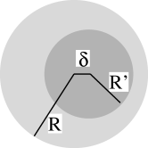
Figure 1: The annular resonator used in the numerical investigations of this paper is composed of two circles with radii $R$ and $R^{\prime}=0.6\,R$, and eccentricity $\delta=0.22\,R$. The refractive index is $n=1$ outside the resonator, $n=1.8$ in the annular region between the circles, and $n=3.3$ inside the interior circle.

II Resonances and quasi-bound states in scattering theory

II.1 Scattering approach

In this paper we apply standard scattering theory to the effectively two-dimensional systems in question. We separate the two polarizations of the electromagnetic field, with either the electric field

$$E_{z}=\operatorname{Re}[\exp(-i\omega t)\psi]$$ (1)

or the magnetic field

$$B_{z}=c^{-1}\operatorname{Re}[\exp(-i\omega t)\psi]$$ (2)

polarized perpendicular to the plane. In both cases, the complex wave function $\psi$ fulfills the two-dimensional Helmholtz equation

$$(\Delta+n^{2}k^{2})\psi=0,$$ (3)

where $n$ is the position-dependent refractive index, $k=\omega/c$ is the wave number, and $c$ is the speed of light in vacuum. Amplification is modelled by a complex refractive index with $\operatorname{Im}n<0$.

We choose a circular region $\cal A$ of radius ${\cal R}>R$, containing the resonator, and decompose the wave function in the exterior of $\cal A$ in the usual Hankel function basis,

$$\psi=\sum_{m}\left(a^{(\rm in)}_{m}H^{(2)}_{m}(kr)+a^{(\rm out)}_{m}H^{(1)}_{m}(kr)\right)e^{im\phi},$$ (4)

where $r$ and $\phi$ are polar coordinates. (Here and in the following, all sums run from $-\infty$ to $\infty$.) The angularly resolved radiation in the far field is given by

$$I(\phi)=\frac{2}{\pi|k|}\left|\sum_{m}a^{(\rm out)}_{m}e^{im(\phi-\pi/2)}\right|^{2}.$$ (5)

Below the laser threshold, the expansion coefficients $a^{(\rm out)}_{m}$ of the outgoing wave are related to their incoming counterparts $a^{(\rm in)}_{m}$ by linear relations

$$a^{(\rm out)}_{m}=\sum_{m^{\prime}}S_{mm^{\prime}}a^{(\rm in)}_{m^{\prime}},$$ (6)

where the coefficients $S_{mm^{\prime}}$ form the scattering matrix. The scattering matrix fulfills the time-reversal symmetry

$$S_{m,n}=S_{-n,-m}(-1)^{m+n},$$ (7)

and is unitary for real $k$ and $n$. For complex values, unitarity is replaced by

$$S^{-1}(k,n)=[S(k^{*},n^{*})]^{\dagger}.$$ (8)

II.2 Poles and quasi-bound states

Quasi-bound states are found at complex values $k_{c}$ of $k$ that permit nontrivial solutions ${\bm{a}}^{(\rm out)}={\bm{a}}_{c}$ in the case of no incident radiation,

$${\bm{a}}^{(\rm in)}={\bm{S}}^{-1}{\bm{a}}^{(\rm out)}=0.$$ (9)

It follows that the values $k_{c}$ are the poles of the scattering matrix, which (for real $n$) all reside in the lower complex plane as a consequence of causality.

For the annular resonator, complex values $k_{c}$ are shown in the bottom panel of Fig. 2, and some typical wave patterns are presented in the right panels of Fig. 3. For this system with a reflection symmetry about the $x$ axis, the quasi-bound states occur with even and odd parity frischat , and further can be divided into whispering-gallery modes localized at the interior interface (class $\rm W_{int}$) or at the exterior interface (class $\rm W_{ext}$), and more extended modes that we group into two classes $\rm A$ (inside the interior circle, these modes are of whispering-gallery character) and $\rm C$ (the remaining modes). Close to resonance in the complex $k$-plane ($k\approx k_{c}^{(\rm even)},k_{c}^{(\rm odd)}$), the scattering matrix can be approximated by petermann2

$$S\approx\frac{{\bm{a}}^{(\rm even)}_{c}\otimes\tilde{\bm{a}}^{(\rm even)}_{c}}{k-k_{c}^{(\rm even)}}+\frac{{\bm{a}}^{(\rm odd)}_{c}\otimes\tilde{\bm{a}}^{(\rm odd)}_{c}}{k-k_{c}^{(\rm odd)}}$$ (10)

where $\tilde{a}_{c,m}=(-1)^{m}a_{c,m}$ due to time-reversal symmetry and we accounted for the potentially quasi-degenerate partner of opposite parity (indicated by the superscripts).

In general, the quasi-bound states found for complex $k_{c}$ and real $n$ can be transported to real values of $k\simeq\operatorname{Re}k_{c}$ by setting $\operatorname{Im}n\simeq\operatorname{Im}k_{c}\operatorname{Re}n/\operatorname{Re}k_{c}$, corresponding to an active, amplifying medium close to threshold remark0 . Above threshold, poles formally move into the upper complex plane, which physically indicates instability, and the linear relation between ${\bm{a}}^{(\rm in)}$ and ${\bm{a}}^{(\rm out)}$ breaks down. Yet, in homogeneously amplifying media the lasing modes are well approximated by the cold-resonator modes laserbooks ; beenakker ; cao . The far-field emission pattern of the laser,

$$I_{c}(\phi)=\frac{2}{\pi|k|}\left|\sum_{m}a^{(\rm out)}_{c,m}e^{im(\phi-\pi/2)}\right|^{2},$$ (11)

is then given by Eq. (5), evaluated with the quasi-bound state ${\bm{a}}_{c}$ that wins the mode competition (the first mode that becomes unstable).

II.3 Resonances and their conventional probes

The values $k_{c}$ are the poles of $S$ where this matrix is singular, and are reflected by resonances of the system at real values $k=\operatorname{Re}k_{c}$. Conventional probes for resonances are obtained from the total scattering cross section

$$\sigma=\frac{4}{k}\sum_{m}|a_{m}^{(\rm out)}-a_{m}^{(\rm in)}|^{2},$$ (12)

and the weighted delay time delaytimes

$$\tau=4\operatorname{Im}\sum_{m}a_{m}^{(\rm out)*}da_{m}^{(\rm out)}/d\omega.$$ (13)

Clearly, the quantities $\sigma$ and $\tau$ depend on the incoming wave, which we now specify as a plane wave coming from direction $\phi_{0}$ remark , corresponding to

$$a^{(\rm in)}_{m}=\frac{1}{2}e^{-im(\pi/2+\phi_{0})}.$$ (14)

Both $\sigma$ and $\tau$ then provide angularly resolved information as a function of $\phi_{0}$. A global characterization of the system is obtained by an average over the incident radiation direction $\phi_{0}$, giving

$$\sigma_{0}=\langle\sigma\rangle_{\phi_{0}}=\frac{1}{k}\sum_{m}(1+\sum_{m^{\prime}}|S_{m^{\prime}m}|^{2}-2\operatorname{Re}S_{mm}),\quad\,\,\,$$ (15)

$$\tau_{\rm W}=\langle\tau\rangle_{\phi_{0}}=\operatorname{Im}\operatorname{tr}S^{\dagger}\frac{dS}{d\omega},$$ (16)

where $\tau_{\rm W}$ is known as the Wigner delay time.

Both the delay time (of predominantly theoretical virtue) and the (more practical) scattering cross section display peaks at resonance, as is illustrated for the annular resonator in the two topmost graphs of Fig. 2. Note that the signal $\sigma_{0}$ is, in general, of low contrast and, apart from a relatively strong background modulation, rather featureless. Still, the enhanced scattering of the light field at resonance promises a marked mechanical response, which we investigate in the remainder of this paper. Indeed, the signal of the mechanical response will display a much better contrast for a set of systematically selected resonances.

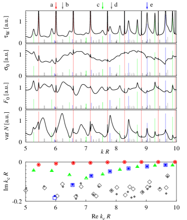
Figure 2: (Color) The top panels show four quantities (in arbitrary units) as a function of $k$ that probe for resonances in the annular resonator: The Wigner delay time $\tau_{\rm W}$, the angle-of-incidence averaged scattering cross section $\sigma_{0}$, the angle-of-incidence averaged force in forward direction $F_{0}$, and the variance of the torque $\operatorname{var}N$. The lower panel shows the complex resonance wave numbers $k_{c}$ of quasi-bound states, classified by their wave patterns as described in the text: ${\rm W}_{\rm int}$ ($\circ$), ${\rm W}_{\rm ext}$ ($\triangle$), ${\rm A}$ ($\Box$), ${\rm C}$ ($\diamond$). Open symbols indicate modes of even parity, full symbols are modes of odd parity. The complex resonances are also indicated by the spikes in the top panels, located at $k=\operatorname{Re}k_{c}$ with height proportional to the life time $1/(-2c\operatorname{Im}k_{c})$. Additionally, the resonances of Fig. 3(a-e) are indicated by the arrows at the very top.

III Mechanical detection of resonances

III.1 Kinematics

In this subsection we provide general kinematic relations for a two-dimensional resonator in a light field, which in the following Subsections III.2,III.3 will be used to characterize resonances and wave patterns.

The mechanical forces exerted by the light field on a dielectric medium originate from the refraction and diffraction at the dielectric interfaces — ultimately, from the deflection (and creation, at finite amplification) of the photons. The kinematics in the combined system of light field and medium can be obtained from the conservation laws of total angular and linear momentum, which equate the torque and force acting on the medium to the deficit of the angular and linear momenta carried by the electromagnetic field into and out of the circular region $\cal A$. (The center of this region is identified with the point of reference for the torque, and in our example is taken as the center of the exterior circle.) Note that the conservation laws also hold in an amplifying medium, due to the recoil of each created photon. The kinematic relations hence follow from integrals of Maxwell’s stress tensor Jackson (1975) over the boundary of $\cal A$. After some algebra (for details see the Appendix), we find the time-averaged force and torque (per unit of thickness of the resonator) in the compact form barton

$$F_{x}+iF_{y} = \frac{2\varepsilon_{0}i}{k}\sum_{m}(a_{m}^{(\rm in)}a_{m+1}^{{(\rm in)}*}-a_{m}^{(\rm out)}a_{m+1}^{{(\rm out)}*}),$$ (17)

$$N = \frac{2\varepsilon_{0}}{k^{2}}\sum_{m}m\left(|a^{(\rm in)}_{m}|^{2}-|a^{(\rm out)}_{m}|^{2}\right).$$ (18)

In absence of amplification and for plane-wave illumination, it is easily seen that the direction-averaged force and torque vanish from the unitarity constraints of the scattering matrix:

$$\langle F_{x}+iF_{y}\rangle_{\phi_{0}}=\frac{-i\varepsilon_{0}}{2k}\sum_{m,m^{\prime}}S_{mm^{\prime}}S^{*}_{m+1,m^{\prime}} = 0,$$ (19)

$$\langle N\rangle_{\phi_{0}}=\frac{\varepsilon_{0}}{2k^{2}}\sum_{m}m\left(1-\sum_{m^{\prime}}|S_{mm^{\prime}}|^{2}\right) = 0.\quad$$ (20)

Two simple quantities that do not vanish are the mean of the force component $F_{\parallel}=F_{x}\cos\phi_{0}+F_{y}\sin\phi_{0}$ in forward direction,

$$F_{0}=\langle F_{\parallel}\rangle_{\phi_{0}}=\frac{\varepsilon_{0}}{2k}\operatorname{Re}\sum_{m,m^{\prime}}(\delta_{mm^{\prime}}-S_{m^{\prime}m}S^{*}_{m^{\prime}+1,m+1}),$$ (21)

and the variance $\operatorname{var}N=\langle N^{2}\rangle_{\phi_{0}}$ of the torque,

$$\operatorname{var}N=\frac{\varepsilon_{0}^{2}}{4k^{4}}\sum_{m,m^{\prime},n_{i}}^{\prime}mm^{\prime}S_{mn_{1}}^{*}S_{mn_{2}}S_{m^{\prime}n_{3}}^{*}S_{m^{\prime}n_{4}}.$$ (22)

Here, the prime at the sum enforces the restriction $n_{1}+n_{3}=n_{2}+n_{4}$.

III.2 Resonances

Because scattering is enhanced at resonance, we expect that $\operatorname{var}N$ and $F_{0}$ are global characteristics of the resonances comparable to $\sigma_{0}$ and $\tau_{W}$, while $N$ and $F_{\parallel}$ provide angularly resolved information as a function of the incident radiation direction $\phi_{0}$, analogously to $\sigma$ and $\tau$. The results in Figs. 2 and 3 demonstrate this promise to hold true.

Figure 2 shows the global characteristics $\sigma_{0}$, $\tau_{W}$, $\operatorname{var}N$, and $F_{0}$ for the annular resonator as a function of $k$. The plot demonstrates a clear correspondence of the resonant peaks in all four quantities. Evidently, each quantity probes another aspect of the resonances, such that their relative weights are different. As usual, the delay time $\tau_{W}$ displays the largest peaks for the very narrow resonances associated to long-living quasi-bound states. Presently, the longest-living states are those of class $\rm W_{int}$, followed by those of class $\rm W_{ext}$ and $\rm A$, while the states of class $\rm C$ are hardly visible here. The scattering cross section $\sigma_{0}$ displays smaller peaks (sometimes, dips) on a modulated background, and does not provide a distinctive discrimination between the different states.

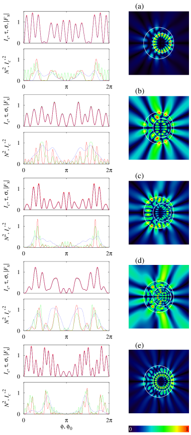
Figure 3: (Color) The panels (a-e) show results for various combinations of $k$ and $\operatorname{Im}n$ tuned very close to resonance with the quasi-bound states of odd parity shown on the right, with (a) $k_{c}=6.009-i\,0.008$ (class $\rm W_{int}$), (b) $k_{c}=6.228-i\,0.116$ (class $\rm C$), (c) $k_{c}=7.554-i\,0.063$ (class $\rm W_{ext}$), (d) $k_{c}=7.847-i\,0.145$ (class $\rm C$), (e) $k_{c}=9.026-i\,0.022$ (class $\rm A$). In the top graph of each panel, the angular dependence of the far field $I_{c}$ (red) on the radiation direction $\phi$ is compared to the angular dependence on the illumination direction $\phi_{0}$ (note Ref. remark ) of the scattering cross section $\sigma$ (green), the weighted delay time $\tau$ (blue), and the $x$-component of the force, $F_{x}$ (purple) — the four lines are almost indistinguishable. In the bottom graph of each panel, the (squared) torque $N^{2}$ (red) is compared to the interference term $I_{c}^{\prime 2}$ (green), defined in Eq. (25). The blue curve is $N^{2}$ evaluated at real $n$. All quantities are in arbitrary units.

The force and torque are sensitive to the wave pattern itself, and for the annular resonator display a marked response especially for the quasi-bound states of class $\rm W_{ext}$ and $\rm A$ (for small $k$, also for class $\rm C$). The peak-to-valley ratio in the variance of the torque (e.g., $\approx 5$ for the peak at $k\approx 6.2$) can take much larger values than in the scattering cross section (where the ratio rarely exceeds 1.2) for resonances with a rather anisotropic internal wave pattern.

This principal conclusion of the present paper is supported in more detail by the five examples in Fig. 3. The wave patterns shown in the right panels are inhomogeneous to various extent, even though the inhomogeneity does not automatically translate into very anisotropic far-field emission patterns for these rather low values of $\operatorname{Re}k_{c}R$. Let us inspect the associated resonance peaks in Fig. 2. For the quasibound state of Fig. 3(a), force, torque, and scattering cross section detect the resonance with comparable contrast; the best signal is given by the delay time, which, however, must be remembered to be an inconvenient tool for practical considerations. Figure 3(b) pertains to a comparatively short-living mode (with large $|\operatorname{Im}k_{c}|$). This mode is hard to detect by the conventional probes, but gives a very clear signal in the mechanical probes, especially, in the torque. For the case of Fig. 3(c), the best signals are provided by the force and by the delay time, followed by the scattering cross section, while the torque is insensitive to this resonance. The case of Fig. 3(d) illustrates that resonances with both a short life time and a rather homogeneous wave pattern are hardly detected by any of the four probes — such modes, however, are also of subordinate interest in the practical applications. The mode of Fig. 3(e) gives a torque signal with a much higher contrast than the force or the scattering cross section; only the delay time signals the resonance to a similar extent.

The most remarkable difference in Fig. 3 is between panels (b) and (d) — both modes of class C displayed there have a short life time, which inhibits their detection by conventional means, but the mode of panel (b) is detectable by opto-mechanical means, in keeping with the larger anisotropy displayed by its wave pattern (note the regions of concentrated intensity above and below the interior circle).

III.3 Far field

In the practical application of micro-optical lasers, the anisotropy of the internal wave pattern is a desired design goal since it is the pre-requisite for directed emission in the far field. To which extent can the far field be inferred from the angularly resolved information contained in $N$, $F$, $\sigma$, and $\tau$? This rather innocent question turns out to be surprisingly subtle in view of the following observation: In absence of amplification (real $k$ and $n$), the angle-of-incidence averaged far field

$$I_{0}(\phi)=\langle I(\phi)\rangle_{\phi_{0}}$$ (23)

is independent of $\phi$. Here, we average over the angle of incidence $\phi_{0}$ since the quasi-bound states are defined without reference to any excitation mechanism. The angle of incidence $\phi_{0}$ enters the far field (5) via Eq. (14), and after taking the average the statement above follows from the unitarity of the scattering matrix. In other words, in the absence of amplification, the angle-of-incidence averaged far-field radiation pattern does not carry any intrinsic information about the quasi-bound states, even at resonant conditions.

Can the far field of the quasi-bound states be inferred from a more sophisticated analysis of $I(\phi;\phi_{0})$, i.e., by taking the dependence of the angle of incidence into account? This would require the delicate task to discard the component of the light that is directly reflected at the first encounter of the boundary from the outside. The direct contribution is essentially independent of the quasi-bound states: the latter are determined by a constructive-interference condition for reflection from the inside of the system while the directly reflected radiation never ever enters the medium. For instance, in our model system, the directly reflected wave component contains no information on the interior circle, which, however, is crucial in the formation of all quasi-bound states.

The situation changes significantly at finite amplification: Then, already the angle-of-incidence averaged intensity $I_{0}(\phi)$ is modulated, and is influenced by the quasi-bound states closest in $k$. At exact resonance in the complex $k$-plane, approximation (10) of the scattering matrix entails ${\bm{a}}^{(\rm out)}\propto{\bm{a}}_{c}$ with a large proportionality constant due to the resonant denominator. Hence the contribution ${\bm{a}}^{(\rm in)}$ of the incident radiation can be neglected, and $I(\phi)\propto I_{c}(\phi)$ as defined in Eq. (11), independent of the mode of excitation. Furthermore

$$\sigma(\phi_{0})\propto\tau(\phi_{0})\propto|F_{x}(\phi_{0})|\propto I_{c}(\phi=\phi_{0}),$$ (24)

since again ${\bm{a}}^{(\rm out)}\propto{\bm{a}}_{c}$ dominates over ${\bm{a}}^{(\rm in)}$ in Eqs. (12), (13), (17). Equation (24) entails a duality between the illumination direction $\phi_{0}$ and the radiation direction $\phi$. This duality relies on the time-reversal symmetry remark , which is incorporated in Eq. (10) by the relation between ${\bm{a}}_{c}$ and $\tilde{\bm{a}}_{c}$. For a representative set of resonances at real $k$ and complex $n$, the far field $I_{c}(\phi)$ is shown in the left panels of Fig. 3, along with the angular dependence of $\sigma$, $\tau$, $|F_{x}|$, and $N$ on the direction of incident radiation, $\phi_{0}$. The wave pattern of the corresponding quasi-bound states is shown in the right panels.

Due to the reflection symmetry of the annular resonator about the $x$ axis, $|F_{y}|\ll|F_{x}|$ while $F_{||}\approx\cos(\phi_{0})F_{x}$. The reflection symmetry also suppresses $N$ compared to non-symmetric systems: The otherwise dominant contribution from ${\bm{a}}^{(\rm out)}={\bm{a}}_{c}$ vanishes for each given quasi-bound state, $\sum_{m}m|a_{c,m}|^{2}=0$, because of pairwise cancellation of the terms with opposite $m$. However, $N$ is still enhanced compared to the non-resonant situation: A non-vanishing result (of order $|k-k_{c}|^{-1}$) is obtained from the interference between the resonant state (with large coefficients) and the non-resonant states (with moderate coefficients). In the typical case of quasi-degeneracy, ${\bm{a}}^{\rm(even)}_{c}$ interferes with ${\bm{a}}^{\rm(odd)}_{c}$, and from Eq. (10) we obtain

$$N^{2}(\phi_{0})\propto I_{c}^{\rm(even)}(\phi_{0})I_{c}^{\rm(odd)}(\phi_{0})\equiv I_{c}^{\prime 2}(\phi_{0}).$$ (25)

This relation is indeed obeyed to good extent in the numerical computations (see Fig. 3). Even at real $n$, $N^{2}$ (the blue curve in the bottom graph of each panel) roughly corresponds to $I_{c}^{\prime 2}$. In non-symmetric geometries the sum $\sum_{m}m|a_{c,m}|^{2}\neq 0$ for a given quasi-bound state, and hence the proportionality $N\sim I_{c}$ (and $F_{y}\sim I_{c}$) is restored (moreover, quasi-degeneracies are then lifted, and the system more easily is tuned to resonance with individual quasi-bound states).

IV Conclusions

In summary, the force and torque exerted by light pressure on a dielectric resonator allow to detect resonances and help to characterize the wave patterns of the associated quasi-bound states. For anisotropic wave patterns that support a high angular-momentum transfer, the peak-to-valley ratio in the mechanical probes (notably the torque) exceeds by far the moderate values observed in the scattering cross section, which is notoriously insensitive to the wave pattern.

We put our work in the context of directed transmission from micro-optical lasers, and took amplification into account. Enhanced sensitivity to internal structure is also desired in several applications involving simpler passive or absorbing media, such as cells with organelles or liquid drops polluted with inclusions.

Since resonance provides a very effective scattering mechanism by constructive interference, the typical forces and torques estimated for common micrometer sized dielectric resonators under typical radiation conditions are in the range of the opto-mechanical experiments mentioned in the introduction. In the viscous rotation experiments, the resonances will depend on the refractive index of the surrounding liquid, which may not be desirable for a precise characterization of the resonator, but also introduces an additional potentially useful control parameter. Detection by microelectromechanical systems offers the advantage to control the resonator orientation with respect to the incoming radiation.

The numerical part of this work concentrated on the wave-optical regime, in which the wave length is not much smaller than the geometric features of the system and interference patterns are most complex. Some micro-optical lasers operate at smaller wave lengths (larger values of the wave number $k$) than accessed in our numerics. In this regime, semiclassical relations between the internal wave pattern and the far-field emission pattern can be formulated, which also relate the directed emission desired for micro-optical laser to the underlying anisotropy of the internal wave pattern. The results of this work hold the promise that in this semiclassical regime, modes with directed emission can be identified by the torque. The selectivity of the torque for anisotropic modes should be even enhanced for these larger values of $k$ by the following mechanism: Isotropic modes frequently arise from a large collection of unstable ray trajectories Gutzwiller (1990), and can be described as a superposition of random waves Berry (1977). As $k$ is increased, more and more random-wave components become available, and hence the mechanical response is suppressed by self-averaging. Anisotropic modes are guided by just a few trajectories such that the self-averaging mechanism does not apply to them, and consequently they remain well detectable by their opto-mechanical response.

*

Appendix A Derivation of the kinematical relations

The calculation of the force

$${\bf F}=\int_{S}dS\,{\bf n}T$$ (26)

and the torque

$${\bf N}=\int_{S}dS\,({\bf n}T)\times{\bf r}$$ (27)

(where $\bf n$ is the unit vector in normal direction to the surface $S$) starts with the stress tensor

$$T=\varepsilon_{0}({\bf E}\otimes{\bf E}-\frac{1}{2}E^{2}\openone)+\frac{1}{\mu_{0}}({\bf B}\otimes{\bf B}-\frac{1}{2}B^{2}\openone).$$ (28)

In the two-dimensional case, we integrate over the circle $\partial A$ of radius ${\cal R}$ (the physical force and torque are obtained by a multiplication with the thickness of the sample), and it is natural to work in polar coordinates.

Depending on the polarization, we insert the electromagnetic field

$$\left.\begin{array}[]{l}{\bf E}=\operatorname{Re}e^{-i\omega t}\psi{\bf e}_{z},\\ {\bf B}=\operatorname{Im}\omega^{-1}e^{-i\omega t}({\cal R}^{-1}\partial_{\phi}\psi{\bf e}_{r}-\partial_{r}\psi{\bf e}_{\phi}),\end{array}\right\}\quad\mbox{(TM)},$$ (31)

$$\left.\begin{array}[]{l}{\bf B}=c^{-1}\operatorname{Re}e^{-i\omega t}\psi{\bf e}_{z},\\ {\bf E}=-c\operatorname{Im}\omega^{-1}e^{-i\omega t}({\cal R}^{-1}\partial_{\phi}\psi{\bf e}_{r}-\partial_{r}\psi{\bf e}_{\phi}),\end{array}\right\}\quad\mbox{(TE)},$$ (34)

where the wave function fulfills the Helmholtz equation (3) and is decomposed in the basis of Hankel function, Eq. (4).

After a time-average, the radial component of the stress tensor then is given in terms of $\psi$ by

$${\bf n}T = \frac{\varepsilon_{0}}{4}\left[(Z^{-2}|\partial_{\phi}\psi|^{2}-|\psi|^{2}-|\partial_{Z}\psi|^{2}){\bf e}_{r}\right.$$ (36)

$$\left.-2Z^{-1}\operatorname{Re}\partial_{\phi}\psi\partial_{Z}\psi^{*}{\bf e}_{\phi}\right],$$

with $Z=k{\cal R}$, $\partial_{Z}=\partial_{kr}|_{r={\cal R}}$, $k=\omega/c$, $c=1/\sqrt{\mu_{0}\varepsilon_{0}}$. (Note that $k$ is real and $n=1$ on $\partial A$, since refraction and amplification is restricted to the resonator.)

The force components can now be expressed as

$$F_{x}+iF_{y} = \frac{\varepsilon_{0}{\cal R}}{4}\int_{0}^{2\pi}d\phi e^{i\phi}\left(\frac{1}{Z^{2}}|\partial_{\phi}\psi|^{2}-|\partial_{Z}\psi|^{2}\right.$$ (37)

$$\left.-|\psi|^{2}-\frac{i}{Z}\partial_{\phi}\psi\partial_{Z}\psi^{*}-\frac{i}{Z}\partial_{\phi}\psi^{*}\partial_{Z}\psi\right).\qquad$$

Here we insert Eq. (4) [indices $m,j$ for $\psi$, indices $m^{\prime},j^{\prime}$ for $\psi^{*}$, where the second index $j,j^{\prime}=(1)\equiv\rm out$ or $(2)\equiv\rm in$] and integrate over $\phi$. Next, we use the identities

$$\partial_{Z}H_{m}^{j} = \frac{m}{Z}H_{m}^{j}-H_{m+1}^{j},$$ (38)

$$\partial_{Z}H_{m+1}^{j^{\prime}*} = -\frac{m+1}{Z}H_{m+1}^{j^{\prime}*}+H_{m}^{j^{\prime}*}$$ (39)

(here and in the following, we suppress the argument $Z$ of the Hankel functions). This gives

$$F_{x}+iF_{y} = \frac{\pi\varepsilon_{0}{\cal R}}{2}\sum_{m,j,j^{\prime}}a_{m}^{j}a_{m+1}^{j^{\prime}*}$$ (40)

$$\left[\Big{(}H_{m+1}^{j}-\frac{m}{Z}H_{m}^{j}\Big{)}\Big{(}H_{m}^{j^{\prime}*}-\frac{m+1}{Z}H_{m+1}^{j^{\prime}*}\Big{)}\right.$$

$$+\frac{m(m+1)}{Z^{2}}H_{m}^{j}H_{m+1}^{j^{\prime}*}-H_{m}^{j}H_{m+1}^{j^{\prime}*}$$

$$-\frac{m+1}{Z}\left(\frac{m}{Z}H_{m}^{j}-H_{m+1}^{j}\right)H_{m+1}^{j^{\prime}*}$$

$$\left.+\frac{m}{Z}H^{j}_{m}\left(-\frac{m+1}{Z}H_{m+1}^{j^{\prime}*}+H_{m}^{j^{\prime}*}\right)\right].$$

Between the square brackets, most terms cancel, giving

$$F_{x}+iF_{y} = \frac{\pi\varepsilon_{0}{\cal R}}{2}\sum_{m,j,j^{\prime}}a_{m}^{j}a_{m+1}^{j^{\prime}*}A_{j,j^{\prime}},$$

$$A_{j,j^{\prime}} = \left(H_{m+1}^{j}H_{m}^{j^{\prime}*}-H_{m}^{j}H_{m+1}^{j^{\prime}*}\right).$$ (41)

With $H^{(1)*}=H^{(2)}$ and the identities

$$A_{11}=-A_{22}=2i\operatorname{Im}H_{m+1}^{(1)}H_{m}^{(2)}=-\frac{4i}{\pi Z},$$ (42)

$A_{12}=A_{21}=0$, we arrive at the final expression (17).

The calculation for the torque is less involved. We find

$${\bf N} = \int d\phi\frac{\varepsilon_{0}{\cal R}}{2k}\operatorname{Re}\partial_{\phi}\psi\partial_{Z}\psi^{*}{\bf e}_{z}$$ (43)

$$= \frac{\pi\varepsilon_{0}{\cal R}}{k}{\bf e}_{z}\operatorname{Im}\sum_{m=-\infty}^{\infty}m$$

$$\left(a^{(1)*}_{m}H^{(2)}_{m}+a^{(2)*}_{m}H^{(1)}_{m}\right)$$

$$\left(a^{(2)}_{m}H^{(2)\prime}_{m}+a^{(1)}_{m}H^{(1)\prime}_{m}\right).$$

The final result (18) follows from $H^{(1)*}=H^{(2)}$ and

$$\operatorname{Im}H_{m}^{(2)}(Z)H_{m}^{(1)\prime}(Z)=\frac{2}{\pi Z}.$$ (44)

References

- Yamamoto and Slusher (1993) Y. Yamamoto and R. Slusher, Phys. Today 46, 66 (1993).
- Vietze et al. (1998) U. Vietze, O. Krauss, F. Laeri, G. Ihlein, F. Schüth, B. Limburg, and M. Abraham, Phys. Rev. Lett. 81, 4628 (1998).
- Qian et al. (1986) S. X. Qian, J. B. Snow, H. M. Tzeng, and R. K. Chang, Science 231, 486 (1986).
- Gmachl et al. (1998) C. Gmachl, F. Capassa, E. E. Narimanov, J. U. Nöckel, A. D. Stone, J. Faist, D. L. Sivco, and A. Y. Cho, Science 280, 1556 (1998).
- (5) Beyond Breit-Wigner theory, the weight also carries information about the non-orthogonality of the right and left eigenmodes of the non-hermitian operator describing the open system; see Ref. petermann2 .
- (6) See e.g. A. Ashkin, Proc. Natl. Acad. Sci. USA 94, 4853 (1997); IEEE J. Select. Topics Quantum Electron. 6, 841 (2000).
- (7) L. Allen, M. W. Beijersbergen, R. J. C. Spreeuw, and J. P. Woerdman, Phys. Rev. A 45, 8185 (1992).
- (8) A. Yamamoto and I. Yamaguchi, Japan. J. Appl. Phys. 34, 3104 (1995).
- (9) M. E. J. Friese, J. Enger, H. Rubinsztein-Dunlop, and N. R. Heckenberg, Phys. Rev. A 54, 1593 (1996).
- (10) E. Higurashi, R. Sawada, and T. Ito, Appl. Phys. Lett. 72, 2951 (1998); Phys. Rev. E 59, 3676 (1999).
- (11) P. Galajda and P. Ormos, Appl. Phys. Lett. 78, 249 (2001); J. Opt. B: Quantum Semiclass. Opt. 4, S78 (2002); Optics Express 11, 446 (2003).
- (12) E. Santamato, A. Sasso, B. Piccirello, and A. Vella, Optics Express 10, 871 (2002).
- (13) Z.-P. Luo, Y.-L. Sun, and K.-N. An, Appl. Phys. Lett. 76, 1779 (2000).
- (14) T. A. Nieminen, N. R. Heckenberg, and H. Rubinsztein-Dunlop, Journal of Modern Optics 48, 405 (2001).
- (15) A. I. Bishop, T. A. Nieminen, N. R. Heckenberg, and H. Rubinsztein-Dunlop, Phys. Rev. Lett. 92, 198104 (2004).
- (16) A. I. Bishop, T. A. Nieminen, N. R. Heckenberg, and H. Rubinsztein-Dunlop, Phys. Rev. A. 68, 033802 (2003).
- (17) J. Moreland, J. Phys. D: Appl. Phys. 36, R39 (2003).
- Bohigas et al. (1993) O. Bohigas, D. Boosé, R. Egydio de Carvalho, and V. Marvulle, Nulc. Phys. A 560, 197 (1993).
- Hentschel and Richter (2002) M. Hentschel and K. Richter, Phys. Rev. E 66, 056207 (2002).
- Wiersig (2003) J. Wiersig, J. Opt. A: Pure Appl. Opt. 5, 53 (2003).
- (21) The splitting of the almost-degenerate pairs of whispering-gallery modes is related to the dynamical tunneling investigated in E. Doron and S. D. Frischat, Phys. Rev. Lett. 75, 3661 (1995); G. Hackenbroich and J. U. Nöckel, Europhys. Lett. 39, 371 (1997).
- (22) H. Schomerus, K. M. Frahm, M. Patra, and C. W. J. Beenakker, Physica A 278, 469-496 (2000).
- (23) The values are slightly shifted, since there is no amplification outside the medium.
- (24) A. E. Siegmann, Lasers (University Science Books, Mill Valley, CA, 1986).
- (25) T. Sh. Misirpashaev and C. W. J. Beenakker, Phys. Rev. A 57, 2041 (1998); M. Patra, Phys. Rev. A 65, 043809 (2002).
- (26) For inhomogeneous media, see H. Cao et al., Phys. Rev. B 67, 161101 (2003); M. Patra, Phys. Rev. E 67, 065603 (2003); L. I. Deych, e-print cond-mat/0306538 (2003).
- (27) F. T. Smith, Phys. Rev. 118, 349 (1960); Y. V. Fyodorov and H.-J. Sommers, J. Math. Phys. 38, 1918 (1997); A. Z. Genack, P. Sebbah, M. Stoytchev, and B. A. van Tiggelen, Phys. Rev. Lett. 82, 715 (1999).
- (28) Note that is the direction to the light source, i.e., the incoming field actually propagates in direction . With this definition, and indeed denote directions related by time-reversal symmetry.
- Jackson (1975) J. D. Jackson, Classical Electrodynamics (John Wiley & Sons, New York, 1975).
- (30) For formulas applying to spheres, see J. P. Barton, D. R. Alexander, and S. A. Schaub, J. Appl. Phys. 66, 4594 (1989).
- Gutzwiller (1990) M. C. Gutzwiller, Chaos in Classical and Quantum Mechanics, vol. 1 of Interdisciplinary Applied Mathematics (Springer, Berlin, 1990).
- Berry (1977) M. V. Berry, J. Phys. A 10, 2083 (1977).