An Object-Oriented Approach to Partial Wave Analysis

Abstract

Partial Wave Analysis has traditionally been carried out using a set of tools handcrafted for each experiment. By taking an object-oriented approach, the design presented in this paper attempts to create a more generally useful, and easily extensible, environment for analyzing many different type of data.

1 Introduction

Partial Wave Analysis, or PWA, is a technique used in hadron spectroscopy to extract information about the spin-parity and decay properties of resonances produced in hadronic interactions. Typically, these resonances are produced at accelerator experiments via a variety of production mechanisms. The resonances produced by these methods also appear in the decay products of other well known resonances, such as the $J/\psi$, and can be studied there. Although the tools we describe here could be used in an investigation that uses any of these production mechanisms, perhaps with slight modification, they have been used extensively only in peripheral production experiments, and so we will use this type of production as an illustrative example in this paper. Currently, new results are being obtained studying baryon resonances produced in $s$-channel $\gamma p$ interactions.

The general idea is to parameterize the intensity distribution in terms of variables that have physical meaning when interpreted as properties of intermediate states in a particular reaction. In principle, any complete set of functions which span the appropriate space can be used. Although many parameterizations are possible, for instance an (almost) purely mathematical description in terms of the moments, we choose an expansion in terms of intermediate resonances and their decays. This has at least two advantages. Firstly, it allows us to take advantage of physics such as conservation laws to limit the number of terms we must include in our expansion to get a good description of the intensity distribution. Secondly, it allows a more direct interpretation of our results. A moment analysis, for instance, requires a complicated mapping from moments to physical states to understand the results in all but the simplest of cases.

The formalism we have used in implementing our system is based on the papers of Chung [1] and Chung and Trueman. [2] The intensity distribution is written as a sum of amplitudes, squared appropriately to account for interference:

$$I(\tau)~{}=~{}\sum_{\alpha}\left\{\left|\sum_{\beta}{}^{\alpha}\psi_{\beta}\left(\tau\right)\right|^{2}\right\}.$$ (1)

The variable $\tau$ represents the set of variables necessary to define a configuration of the final state being investigated. It typically includes the angles of the decay products in various reference frames, masses of two body sub-systems, etc. The subscripts $\alpha$ and $\beta$ are the parameters that describe the partial wave decomposition we are using, $\alpha$ specifying properties of the different intermediate states that do not interfere, such as the spin states of the incoming or outgoing particles in the detector. The subscript $\beta$, on the other hand, represents the properties whose differing values do interfere, for instance the spin states of broad resonances produced as intermediate states in a sequential decay.

In a peripheral production experiment, the amplitudes in the expansion can be drawn as shown in Fig. 1.

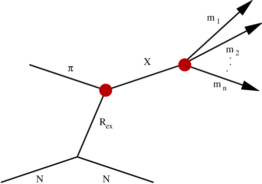
Figure 1: Diagram representing the amplitude $\psi_{\alpha\beta}\left(\tau\right)$. The intermediate state $X$ is produced by the exchange of a Reggion $R_{ex}$ between the $\pi$ beam and the nucleon target.

Guided by this picture, the amplitude $\psi_{\alpha\beta}\left(\tau\right)$ is factored into two parts: $V$, the amplitude to produce the state $X$, and $A$, the amplitude for the state $X$ to decay into the final state observed.

These amplitudes are written in the reflectivity basis [2], which takes into account parity conservation in the production process by writing the amplitudes in terms of eigenstates of reflection through the production plane. The reflectivity of the amplitude, denoted $\epsilon$, is defined so that in the case of a pion beam it coincides with the naturality of the exchanged Regge trajectory. Waves of differing $\epsilon$ do not interfere. Also, amplitudes with different relative spin configurations for the incoming and outgoing baryon will not interfere. The spin configuration of the amplitudes is labeled by $k$, and the number of allowed values, sometimes referred to as the rank of the fit, is typically 2 for a spin ${\textstyle\frac{1}{2}}$ recoil baryon.

In the reflectivity basis our sum over amplitudes splits into four non-interfering sets of fully interfering amplitudes, or $\alpha~{}=~{}\left\{\epsilon,k\right\}$. While both the production and decay amplitudes depend on $\epsilon$, the decay amplitude does not depend on $k$, since the decay amplitude for a particular state $X$ cannot depend on what the proton spin did during the production process. Similarly, the production amplitude does not depend on $\tau$, the configuration of the final state the $X$ decays into.

The intensity distribution now becomes

$$I\left(\tau\right)~{}=~{}\sum_{\epsilon,k}\left\{\left|\sum_{\beta}{}^{\epsilon}V_{k\beta}{}^{\epsilon}A_{\beta}\left(\tau\right)\right|^{2}\right\}.$$ (2)

The decay amplitudes ${}^{\epsilon}A_{k\beta}\left(\tau\right)$ can be calculated for each event. By varying the unknown production amplitudes ${}^{\epsilon}V_{k\beta}$ the predicted intensity distribution above is matched as closely as possible by the observed intensity as a function of all kinematic variables. This is done through an extended maximum likelihood fit. During the fitting process, the finite acceptance of the detector is taken into account on a term by term basis, i.e., each term contains a pair of of decay amplitudes with a unique shape in $\tau$, and the acceptance for each term is determined separately.

The likelihood function is defined as a product of probabilities,

$$\mathcal{L}=\left[{\bar{n}^{n}\over{n!}}e^{-\bar{n}}\right]\prod_{i}^{n}\left[{I(\tau_{i})}\over{\int(\tau)\eta(\tau)d\tau}\right]$$ (3)

The term outside the product is the Poisson probability of observing $n$ events and reflects the fact that we use the extended maximum likelihood method. The integral in the denominator of the summed term contains the acceptance $\eta(\tau)$ and is referred to as the accepted normalization integral.

The function which is actually maximized in the likelihood fit is

$$\ln{\mathcal{L}}=\sum_{i}^{n}\left[\ln\sum_{k,\epsilon,\beta,\beta^{\prime}}{}^{\epsilon}V_{k\beta}{}^{\epsilon}V_{k\beta^{\prime}}^{*}{}^{\epsilon}A_{\beta}(\tau_{i}){}^{\epsilon}A_{\beta^{\prime}}^{*}(\tau_{i})\right]-n\left[\sum_{k,\epsilon,\beta,\beta^{\prime}}{}^{\epsilon}V_{k\beta}{}^{\epsilon}V_{k\beta^{\prime}}^{*}{}^{\epsilon}\Psi_{\beta\beta^{\prime}}^{x}\right]$$ (4)

The first sum is over data events, where the term being summed over is simply the intensity $I(\tau_{i})$ for each event. The second term contains the accepted normalization integrals ${}^{\epsilon}\Psi^{x}_{\beta\beta^{\prime}}$ where the superscript $x$ denotes accepted. This integral is evaluated numerically:

$${}^{\epsilon}\Psi^{x}_{\beta\beta^{\prime}}={1\over M_{x}}\sum_{i}^{M_{x}}{}^{\epsilon}A_{\beta}(\tau_{i}){}^{\epsilon}A^{*}_{\beta^{\prime}}(\tau_{i}).$$ (5)

The sum is over an accepted Monte-Carlo data set of $M_{x}$ events. A similar integral is calculated for the raw Monte-Carlo data set, to be used in the calculation of observables. For instance, the number of acceptance corrected events the fit predicts is

$$N={n\over{\eta_{x}}}\sum_{\epsilon k\beta\beta^{\prime}}{}^{\epsilon}V_{k\beta}{}^{\epsilon}V^{*}_{k\beta^{\prime}}{}^{\epsilon}\Psi_{\beta\beta^{\prime}},$$ (6)

where ${}^{\epsilon}\Psi_{\beta\beta^{\prime}}$ is the raw normalization integral. By varying the range of the values of $\left\{\epsilon k\beta\beta^{\prime}\right\}$ included in the sum, the number of events due to different combinations of amplitudes can be determined.

1.1 Decay Amplitudes

Calculation of decay amplitudes for the resonance $X$ is done recursively using the isobar model, regarding the $n$-body final state as the result of a series of sequential decays (usually two body) through intermediate states known as the isobars. The amplitude for $X$ to decay into the final state is then simply the amplitude for $X$ to decay into its immediate children times the amplitude for each of its children to decay.

The initial decay of the $X$ into its children is evaluated in the Gottfried-Jackson frame. This frame is a rest frame of the resonance $X$ with the $z$ axis in the direction of the beam and the $y$ axis perpendicular to the production plane. The quantities used in defining the amplitude are shown schematically in Fig. 2

Figure 2: Decay of the resonance $X$ into $x_{1}$ and $x_{2}$.

The state $X$ of mass $W$ has spin $J$ with $z$ projection $m$. It decays into children $x_{i}$ with spin $\sigma_{i}$ and helicity $\lambda_{i}$. These children have a breakup momentum $\vec{p}$ and relative orbital angular momentum $\ell$. The decay amplitude can then be written down [3]

$$A_{X}=\tilde{\ell}\sum_{\lambda}D^{J*}_{m\lambda}(\Omega)(\ell 0s\lambda|J\lambda)(s_{1}\lambda_{1}s_{2}-\lambda_{2}|s\lambda)F_{\ell}(p)a_{\ell s}A_{x_{1}}A_{x_{2}}$$ (7)

where $\lambda=\lambda_{1}-\lambda_{2}$ and $\vec{s}=\vec{s}_{1}+\vec{s}_{2}$, i.e. , $\vec{s}$ is the total spin of the two children and $\lambda$ is the component of $\vec{s}$ in the direction defined by $x_{i}$’s momentum. The $A_{x_{i}}$ are the decay amplitudes of each child.

The $\tilde{\ell}=(2\ell+1)^{{\textstyle\frac{1}{2}}}$ factor, along with the two Clebsch-Gordon coefficients, come from the fact that we are using helicity states and must relate the helicity coupling constant to the $\ell s$-coupling constant, $a_{\ell s}$, we want to find through the partial wave expansion.[3]

Rotational properties of the helicity states lead to the introduction of $D$-function $D^{J*}_{m\lambda}(\Omega)$ where $\Omega=(\theta,\phi,0)$ are the Euler angles of $x_{1}$ in the Gottfried-Jackson frame. The choice of the third angle $\gamma$ defines the phase convention. We choose $\gamma=0$, which is different from that of Jacob and Wick [4], who choose $\gamma=-\phi$.

$F_{\ell}(p)$ is an angular momentum barrier factor added to give the amplitude the correct behavior near threshold. We used the Blatt-Weisskopf centrifugal-barrier functions as given by von Hippel and Quigg. [5]

Finally, $a_{\ell s}$ is the $\ell s$ coupling constant which contains the dynamics of the decay. This factor is absorbed into the production amplitude for this wave, which is then determined through the fit. The coupling constant $a_{\ell s}$ is in general a function of the mass $W$ of the state $X$, and this is usually handled in the fits by performing them in bins of $W$ which are narrow enough to assume the $a_{\ell s}$ constant over the width of the bin.

The decay amplitudes of the children $A_{x_{i}}$, and recursively their children, etc., are calculated in the helicity frame of the child that is decaying. For instance, consider one of the $x_{i}$ above, but now we call it simply $x$ since it has become the parent particle of a new decay, as in Fig. 3

Figure 3: Decay of a child $x$ into $x_{1}$ and $x_{2}$.

Here the particle decaying, $x$ has mass $w$, spin $s$, and helicity $\lambda$. Its decay products $x_{i}$ have spins $\sigma_{i}$ and helicities $\nu_{i}$, with relative orbital angular momentum $\ell$ and breakup momentum $p$.

The form of the amplitude for this piece of the decay is very similar to what was written above

$$A_{x}=\tilde{\ell}\sum_{\lambda}D^{s*}_{\lambda\nu}(\Omega)(\ell 0\sigma\nu|s\nu)(\sigma_{1}\nu_{1}\sigma_{2}-\nu_{2}|s\nu)F_{\ell}(p)\Delta_{x}(w)A_{x_{1}}A_{x_{2}}$$ (8)

where again $\nu=\nu_{1}-\nu_{2}$ and $\vec{\sigma}=\vec{\sigma}_{1}+\vec{\sigma}_{2}$

The pieces of this decay that look similar to the initial decay in the Gottfried–Jackson frame do so because they come from the same place. The same Clebsch–Gordon coefficients and $\tilde{\ell}$ factor show up from the relationship of the helicity to $\ell s$ states, the $D$–function from the rotational properties of the states, and the angular momentum barrier factor suppresses high-$\ell$ decays near threshold where the breakup momentum is small.

The only difference, in fact, is the appearance of $\Delta_{x}(w)$ in place of the coupling constant $a_{\ell s}$ from the initial decay. In the decays of the isobars it is usually assumed that the dynamics of the decay, which depend on the isobar mass $w$, are known and put in explicitly. Often this is done as a simple relativistic Breit-Wigner, although it is sometimes necessary to use a more complex parameterization, such as coupled-channel Breit-Wigners [6] or a $K$–matrix parameterization [7].

Total decay amplitudes are made up as a product of these intermediate decays. In order to parameterize the spin-density matrix, which is determined by the fit, in the simplest way, it turns out to be advantageous to transform the states into the reflectivity basis. The reflectivity basis is defined by eigenstates of reflection in the production plane, the details of the transformation can be found in Chung and Trueman. [2]

2 Choice of Tools

After determining the design criteria from the considerations in the last section, we choose tools to assist in building the system to meet these criteria.

2.1 The choice of language

Choosing a language was not as difficult as one might hope: the paucity of object-oriented languages having the support of adequate development tools led us almost immediately to C++. Java, Eiffel and Sather were briefly considered. Java was decided to still be too slow for numerically intensive calculations. Eiffel and it’s relative Sather are interesting languages that address some of the deficiencies of C++, but the lack or weakness of development tools such as a symbolic debugger led us to pass them up.

C++ is a popular language which now has an ANSI/ISO standard. There are numerous compilers, debuggers, CASE tools and class libraries available. In particular, we choose the GNU compiler suite and development tools. The GNU C++ compiler is very close to the ANSI standard, and since most of our development and analysis is done on a Linux/GNU platform it is also the native compiler on these systems. Using C++ also gives us the advantages of an object-oriented language while also providing convenient access to useful libraries written in C or FORTRAN. For instance the engine of our fitting program is the CERNLIB package MINUIT.

Attempting to deliver a “turnkey” system that, given a physics data set in a standard format, would allow users to perform an analysis implies a relatively sophisticated control language for our tools. Yacc and it’s cousin Lex allowed easy development of a flexible grammar for driving both the decay amplitude calculator and the fitter. These development tools interface very well with C++ and are standard on any *NIX system.

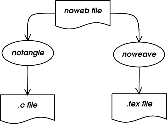
Figure 4: A noweb source file is pre-processed with either notangle or noweave to produce either source code or documentation, respectively.

2.2 The choice of documentation system

In our experience, up to date documentation for software written by physicist is hard to find–our own code has not been an exception. We take the view that self-documenting code is a realizable goal as long as the audience is programmers. For this project we were striving to reach a much broader audience, and hence recognized the need for something else. We decided to use noweb [8], a simple literate programming package.

Literate programming [9] was first proposed by Donald Knuth, which he implemented in the form of web. Essentially code and documentation are written interspersed in the same files, making it easier to document the code as it is written, and encourages the documentation to keep pace with program development. The pre-processors which make up the web system then weave the web file into documentation, usually in latex format, or tangle the web file into source code. While some literate programming tools are language specific, noweb allows any programming language to be embedded into its files, allowing symmetric treatment of C++, yacc, lex, etc.

3 The Design

3.1 The architecture of the suite

The design of the tools is strongly influenced by the mathematics of the fitting, some of which was described above. In general, we felt that a set of independent programs each of which which work with the output of the others is the best design. We clearly need a program to perform the minimization of the $-\ln(\mathcal{L})$ function of equation 4. The normalization integral, equation 5, is calculated prior to fit and requires a program of its own. We must have a program to calculate decay amplitudes as a function of $\tau$. This implies three basic programs are required for an analysis. During the course of testing and use, however, several additional utility programs were written. Some of these turned out to be generally useful and will also be briefly described in this report.

A picture of the entire procedure is shown in Fig. 5.

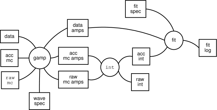
Figure 5: Pictorial view of the entire PWA procedure. The three circles represent the three major computational steps, acting on the rectangular data files.

The decay amplitude calculator gamp computes the decay amplitude given an event and a particular “wave”: an assumed spin-parity for the whole system, any isobars with their spin-parities, and a orbital angular momentum and total spin for each two body decay. The integrator int, used to compute normalization integrals used in the fitting process, must read amplitudes calculated by gamp and integrate over the appropriate space. The production amplitudes are found by fit using a maximum likelihood fit.

3.2 The architecture of gamp

A typical invocation of the program to generate amplitudes might look like:

zcat data.gamp.gz | gamp 1++0+rho_pi.key > 1++0+rho_pi.amps

Notice that gamp reads and writes from standard input and output, and that it’s single required argument is the name of a keyfile, a program specifying the amplitude to be calculated for each event read from it’s input. gamp uses an awk-like processing model: the program in the keyfile is run repeatedly on each event as it is read in. The language of this program is described below.

3.2.1 Event format

The format of the events read from standard input is quite simple. The events are expected to be in ASCII format. Each event begins with an integer specifying the number of particles which will follow. Particles are given by their GEANT id (integer), their charge (integer), and the four components of their four momentum, $p_{x}$, $p_{y}$, $p_{z}$, $E$ (floats). The first particle in each event is always the beam. Presently, the target is not specified and is assumed to be a proton (this is likely to change in the near future, and the target will be required). Following the beam come all final state particles from the system being analyzed, in arbitrary order, and then the next event, etc.

For example, the top of a file containing events from the reaction $\pi^{-}p\rightarrow p\eta\pi^{+}\pi^{-}\pi^{-}$ might look like

5
9 -1  0.0003765 -0.0573188 18.3642158 18.3648357
9 -1  0.0814732  0.4102049  2.2733631  2.3157212
9 -1  0.2404482  0.3578656  3.9542443  3.9801270
8  1  0.3348054  0.0241324  3.3473827  3.3670651
17 0 -0.4792622 -0.4030199  8.5089292  8.5494852
5
9 -1 -0.0850012 -0.0702078 18.1182842 18.1191577
9 -1 -0.4165566  0.1685560  1.5984030  1.6662241
...

Notice in this example, from BNL E852, the reaction is assumed to be a $t$-channel process. Therefore the system being studied here is $\eta\pi\pi\pi$ and the final state proton does not appear in the input. This is optional, the keyfile specifying the amplitude to calculate will refer to particles by name, unmentioned particles are simply ignored. Thus specifying the proton in the event and ignoring it in the keyfile will not create an error. If an $s$-channel amplitude is being calculated, all final state particles would be required in the event specification.

Since gamp reads events from standard input, these ASCII files can be stored compressed and then zcatted into a pipe. Or better still, never put to disk, but created on the fly from the (presumably) more efficient binary data format of the particular experiment.

3.2.2 The keyfile language

The keyfile language is fairly simple. The file is free-format: spaces, tabs, and newlines may be used to improve readability. Statements are terminated by semi-colons.

A very simple keyfile might look like this:

# debug = 1;
channel = t;
mode = binary;

J = 2 P = +1 M = 2 {
        pi+
        pi-
        l=4
}
;

In this file we are specifying the decay of a state with $J^{P}=1^{+}$ and $m=1$ into two pions with two units of angular momentum between them, i.e., an D wave.

A # comments the remainder of the line. Here the debug = 1;, which would turn on copious debugging information, is commented out. The amplitude being calculated is for a $t$-channel process. The only allowed values for channel are s and t. Amplitudes output can be in either ASCII (default) or binary format, and can be selected by setting mode to either ascii or binary. Finally comes the specification of the wave itself. A wave is a set of quantum numbers–$J$, $P$ and $M$–followed by a decay. Note: all angular momenta are in units of $\hbar/2$, i.e., multiplied by 2. This allows particles with half-integer spin to be represented as integers in the input. In the example above, for instance, the state being calculated has $J^{P}=1^{+}$.

The decay is represented by a pair of child particles followed by the orbital angular momentum between them, and optionally, their total spin. If the total spin is not ambiguous, it may be omitted. Only when both particles have non-zero spin is it necessary to explicitly give the spin, and it must follow the orbital angular momentum. The orbital angular momentum and spin may be labeled as above or may be unadorned integers. The first integer is always the orbital angular momentum and the second, if present is the total spin. The decay specification is delimited by the pair of curly brackets. Although it may be spread out over many lines, the entire wave is a single statement, so don’t forget the ; at the end.

3.2.3 Combining Waves

Waves may be added to eachother, and this gives us a way to handle symmetrizing amplitudes when there are identical particles. If the final state contains identical particles, they are identified in the wave specification as if the identical particles were read into a (1-indexed) array, i.e., pi+[1] is the first positively charged pion read for each event, pi+[2] is the second etc. So to form a Bose-symmetrized amplitude use something similar to the following:

# debug = 1;
channel = t;
mode = binary;

0.707 * (
J = 4 P = +1 M = 0 {
        pi0[1]
        pi0[2]
        l=4
}
+ J = 4 P = +1 M = 0 {
        pi0[2]
        pi0[1]
        l=4
} )
;

In this case the second wave look the same with the exception of the flipped indices on the pi0’s: we have exchanged the two identical particles.

3.2.4 Sequential Decays

Any unstable particle may be followed by a similar decay specification, recursively. For example, gamp would not balk at a decay chain as follows:

# debug = 1;
channel = t;
mode = binary;

J = 2 P = +1 M = 0 {
        a2(1320) {
                rho(770) {
                        pi+[1]
                        pi-[1]
                        l = 2
                }
                pi0
                l = 4
        }
        rho(770) {
                pi+[2]
                pi-[2]
                l = 2
        }
        l = 2
        s = 2
} ;

This keyfile describes a $J^{P}=1^{+}$ particle in an $m=0$ state decaying into $a_{2}\rho$ via a $P$ wave. Notice here that we have included a specification of the total spin of the $a_{2}\rho$ system $s=1$, as it is not unique. The $a_{2}(1320)$ decays further in this example into $\rho\pi$ in a $D$ wave, and finally each $\rho$ decays into $\pi\pi$ with $\ell=1$.

3.2.5 Mass Dependencies

Currently, gamp also understands a few different mass dependencies for isobars: flat, Breit-Wigner, and two solutions for $(\pi\pi)_{S}$. Others will be added by popular demand. The alternate mass dependencies are given by appending, for instance, the statement massdep = flat after the decay, as in

# debug = 1;
channel = t;
mode = binary;

0.707 * (
J = 4 P = +1 M = 0 {
        pi0[1]
        pi0[2]
        l=4
} massdep=flat
+ J = 4 P = +1 M = 0 {
        pi0[2]
        pi0[1]
        l=4
} massdep=flat )
;

The other appropriate keywords are bw for Breit-Wigner (the default), amp for Au-Morgan-Pennington $(\pi\pi)_{S}$ parameterization (M-solution) [10], and amp_ves for VES modification [11, 12] to above.

3.2.6 Helicity Sums

The default action when gamp sees a particle with spin is to sum over the allowed helicities. This is in general the correct action as particles with spin are usually intermediate states which interfere and must be summed over at the amplitude level. Final state particles are typically spinless with the notable exceptions of protons and neutrons. If these appear in the wave specification the amplitude must not be summed over and the helicity or h keyword allows for this.

mode=binary;
channel=s;

0.94868 * (
J=3 P=-1 M=1 {
        delta(1232)[1] {
                p+[1]   h=-1
                pi+[1]
                2
        }
        pi-[1]
        4
}
+ 0.33333 * (
J=3 P=-1 M=1 {
        delta(1232)[1] {
                p+[1]   h=-1
                pi-[1]
                2
        }
        pi+[1]
        4
}
));

This keyfile describes the decay of a $J^{P}={3\over{2}}^{-}$ baryon resonance into $\Delta\pi$ in a $D$ wave. The two charge possibilities for the $\Delta$’s are combined with the correct Clebsch-Gordon coefficients to produce an isospin $1\over 2$ state. This wave is being calculated for the negative helicity of the final state proton; presumably the positive helicity would be calculated also and added incoherently at fit time.

3.3 The architecture of int

The normalization integrals, whose values are needed at the time of the fit, are calculated using int. Recall that the integrals needed look like

$$\Psi_{\alpha\alpha^{\prime}}=\int\psi_{\alpha}^{*}(\tau)\psi_{\alpha^{\prime}}(\tau)\eta(\tau)d\tau~{}=~{}{1\over M}\sum_{i}\psi_{\alpha}^{*}(\tau_{i})\psi_{\alpha^{\prime}}(\tau_{i})$$ (9)

where $d\tau$ is an element of phase space, $\tau$ is then a point in phase space, $\psi_{\alpha}(\tau)$ is the decay amplitude for the wave $\alpha$ as a function of the kinematic variables defining phase space $\tau$. This is an accepted integral, used at fitting time to perform the acceptance correction, and hence the appearance of the acceptance $\eta(\tau)$. Unfortunately, the acceptance of a detector is rarely known analytically, and so this integral is always done numerically. This is shown in the last term as a sum over Monte-Carlo generated events. The generation is done uniformly in phase space, i. e. flat in $\tau$. These events are then passed through a detector simulation program, and subjected to the same analysis and cuts. Using only these $M$ remaining events in the sum above take into account the $\eta(\tau)$ factor in the integral. Similar integrals are needed post-fit to calculate observables from the fit results, as descibed by equation 6. These “raw” integrals differ from the above “accepted” integrals only by their lack of the acceptance term $\eta(\tau)$ in the raw integrals. Numerically this corresponds to performing the sum over the entire generated phase space Monte-Carlo event sample.

int assumes all decay amplitudes $\psi_{\alpha}(\tau_{i})$ are available on disk and a single file holds all amplitudes for a single wave $\alpha$ for each event in a particular data set. All the amplitude files should correspond to the same data set. The integrals $\Psi_{\alpha\alpha^{\prime}}$ are kept internally as matrices. Individual integrals may be accessed by either integer indices of the matrix, or by a string representing the name of the wave–a human readable form of $\alpha$.

3.4 The architecture of fit

In the course of an analysis many fits need to be done. It is important to try different sets of waves in many combinations: two waves may not be important individually, but their interference may be. In addition, once the best set of waves is determined, the stability of the fit can be studied by repeating the fit with varying starting values for the parameters. A completed analysis will often require hundreds of fits.

The likelihood function maximized varies depending on the type of process being modeled. A $s$-channel likelihood function differs from a $t$-channel function, and a photon beam requires a different function from a pion beam. Different assumptions may also be tested with regard to the “rank” of the fit, relating to whether or not the amplitudes have differing dependence on spin degrees of freedom.

The lack of a standard function led to the idea of using an interpreter for the likelihood function. The input file for the fit contains the specification of the likelihood function. A simple example file looks like:

damp 0m0.amps;
damp 1m0.amps;
damp 1p0.amps;
damp 2m0.amps;
damp 2p0.amps;

realpar p0m0;
par p1m0;
par p1p0;
par p2m0;
par p2p0;

integral normInt(normInt.new);

event_loop:
    fcn = fcn - log(
        absSq(p0m0*0m0.amps + p1m0*1m0.amps
            + p1p0*1p0.amps + p2m0*2m0.amps
            + p2p0*2p0.amps)
    );

normalization:
    fcn = fcn + nevents * (
        p0m0*conj(p0m0)*normInt[0m0.amps , 0m0.amps] +
        p1m0*conj(p1m0)*normInt[1m0.amps , 1m0.amps] +
        p1p0*conj(p1p0)*normInt[1p0.amps , 1p0.amps] +
        p2m0*conj(p2m0)*normInt[2m0.amps , 2m0.amps] +
        p2p0*conj(p2p0)*normInt[2p0.amps , 2p0.amps] +

        2.0*real( p0m0*conj(p1m0)*normInt[0m0.amps , 1m0.amps] +
            p0m0*conj(p1p0)*normInt[0m0.amps , 1p0.amps] +
            p0m0*conj(p2m0)*normInt[0m0.amps , 2m0.amps] +
            p0m0*conj(p2p0)*normInt[0m0.amps , 2p0.amps]) +

        2.0*real( p1m0*conj(p0m0)*normInt[1m0.amps , 0m0.amps] +
            p1m0*conj(p1p0)*normInt[1m0.amps , 1p0.amps] +
            p1m0*conj(p2m0)*normInt[1m0.amps , 2m0.amps] +
            p1m0*conj(p2p0)*normInt[1m0.amps , 2p0.amps]) +

        2.0*real( p1p0*conj(p0m0)*normInt[1p0.amps , 0m0.amps] +
            p1p0*conj(p1m0)*normInt[1p0.amps , 1m0.amps] +
            p1p0*conj(p2m0)*normInt[1p0.amps , 2m0.amps] +
            p1p0*conj(p2p0)*normInt[1p0.amps , 2p0.amps]) +

        2.0*real( p2m0*conj(p0m0)*normInt[2m0.amps , 0m0.amps] +
            p2m0*conj(p1m0)*normInt[2m0.amps , 1m0.amps] +
            p2m0*conj(p1p0)*normInt[2m0.amps , 1p0.amps] +
            p2m0*conj(p2p0)*normInt[2m0.amps , 2p0.amps]) +

        2.0*real( p2p0*conj(p0m0)*normInt[2p0.amps , 0m0.amps] +
            p2p0*conj(p1m0)*normInt[2p0.amps , 1m0.amps] +
            p2p0*conj(p1p0)*normInt[2p0.amps , 1p0.amps] +
            p2p0*conj(p2m0)*normInt[2p0.amps , 2m0.amps])
    );

This file shows all the key elements of the fit input file grammar. The statements at the top of the file declare some variables. damp’s are decay amplitudes, the string following is both the filename where the amplitudes for a particular wave are found and the name of the variable that can be used in the function to refer to this wave. par’s are the fit parameters, assumed to be complex unless realpar is specified. Finally, integral normInt(normInt.new); declares normInt to be a normalization integral found in the file normInt.new. The executable statements in the second half of the file are in two sections. The event_loop section is executed for every event in the dataset, while the normalization section is done only once, after the loop over events. fcn is a reserved word that is the value to be minimized by varying the par’s. An astute reader might recognize fcn as a relic of the CERNLIB minuit minimizer, which is in fact the package used to perform the actual minimization. Notice also that the normalization integrals are indexed by the name of the wave, or more precisely, the name of the file that contained the decay amplitudes for that wave at the time of integration.

The interpreter for this file is based heavily on hoc by Kernighan and Pike [13]. Briefly, the file is parsed and statements are stored as instructions to a virtual stack machine which is run at fit time. Decay amplitudes and parameters are stored in a symbol table and their values are updated appropriately: every event for the amplitudes and every iteration of the fitter for the parameters. The code generated for a part of the above event loop, p0m0*0m0.amps + p1m0*1m0.amps is shown in Table 1.

varpush
p0m0
eval
varpush
0m0.amps
eval
mul
varpush
p1m0
eval
varpush
1m0.amps
eval
mul
add

Table 1: Instructions generated by code fragment explained in text.

Most instructions are simply pointers to a corresponding function, therefore execution of the program means simply marching down this list of function pointers, executing each one as you go. Any “instruction” which is not a function pointer should be skipped by the true instruction before it. For instance, the initial varpush in the program shown above pushes the next “instruction”, the variable name p0m0, onto the stack and increments the program counter past the next instruction to the eval that follows it. The eval function pops the top value off the stack, looks it up in the symbol table, and pushes its value back onto the stack. Therefore the first three instructions have the effect of pushing the value of p0m0 onto the stack. The next three instructions similarly push the value of 0m0.amps onto the stack. The stack now contains these two complex numbers, and the mul instruction pops both off the stack, multiplies them, and pushes the result back on the stack.

This produces an extremely flexible fitting program, with two possible drawbacks. The first drawback is the complexity of the input file. Even the simple example given above generates many terms and a realistic fit input using tens of waves could easily require pages of input containing many similar symbols such as file names that differ by one character. To reduce the opportunity for errors to arise, these input files are often written by a separate program. We use a prolog program to generate the fit input files. This program reads the states we wish to include in the fit, produces a list of production amplitudes to be used as fit parameters, and applies any known constraints such as parity conservation to link any amplitudes it can. The resulting list is formatted appropriately for fit to read and output to a file.

The second drawback of an interpreted system is performance. While very flexible, an interpreted system is inherently slower. In recent work where this has become an issue, the function written by the prolog program was modified to allow direct compilation by the C++ compiler and was used directly with minuit for fitting.

3.5 Description of libpp classes

We have gathered into libpp a collection of classes that were of general use in particle physics, beyond the specialized topic of partial wave analysis. This section is not an attempt to fully document this library, but rather just a sampling of a few of the objects available to give the flavor of what is found in libpp.a. The complete documentation can be obtained from the source using notangle, or preformatted from the web at http://ignatz.phys.rpi.edu/~cummij/

Three- and four-vectors are defined as threeVec and fourVec, with most common operations available as member functions. The implementation of fourVec’s used contains a threeVec and a double, rather than deriving both from a base vector class. While the implementation details are not assumed in the interface to the class, one can see reflections of the implementation in some of the methods such as the constructors (fourVec(double t, threeVec space), for instance)

A particle data table class particleDataTable is a simple database containing information about known particle states from the Particle Data Groups Review of Particle Properties. It is essentially a list of particleData objects. It is initialized to a default set of values from the 2002 edition of the Review of Particle Properties, but can be modified by reading a local file containing “custom” particles. Lookup in the table is implemented as a linear search, which is not a performance issue for the typical size tables involved. The particle class represents a physical instance of a particle, i. e. a particleData with an associated fourVec. The event class contains the beam, target, and a list of final state particles.

Matrices are implemented as template classes to allow both the matrices of complex numbers used in partial wave analysis and real matrices such as Lorentz transformations to share the same code. Lorentz transformations are derived from the template class matrix<> and can be used to boost fourVec’s, particle’s or event’s. A particularly useful constructor makes a lorentzTransform from a fourVec, defining the transformation to boost into the rest frame of the fourVec, treating it as a four-momentum. This allows convenient constructs such as:

        event e;
        // read the event from standard input
        std::cin >> e;
        lorentzTransform L(e.beam().get4P()+e.target().get4P());
        // put the event into the beam + target rest frame
        e = L*e;

which puts the entire event into the center of mass system.

4 Example analysis

As a demonstration of the flexibility of this system, lets consider the analysis of data from Jefferson Laboratory looking for “missing baryon” states. The experiment collected data from the reaction $\gamma p\to p\pi^{+}\pi^{-}$, with a $\gamma$ beam energy of 0.5-2.6 GeV/$c$. Data were selected which reconstructed all three final state particles, leaving a data sample of 750k events for partial wave analysis. While a complete description of this analysis is beyond the scope of this paper, A brief description of the analysis should illustrate the pwa2000 well.

This is a particularly difficult region to partial wave analyze, due to the fact that the dynamics is expected to change drastically within the range of the analysis. For instance, for beam energies below $\rho$ threshold the data are in the resonance region and will probably be well described by formation of isobars in the $s$-channel. Above $\rho$ threshold the center of mass energy is leaving the resonance region and the availability of the $\rho$ should result in a large contribution from diffractive ($t$-channel) $\rho$ production. The transition between these two kinematic extremes will be difficult to map, and will require many fits trying not only many different sets of waves but also different likelihood functions as we make different assumptions about how to describe $t$-channel processes in a truncated $s$-channel basis. It is for exactly this situation that we designed a flexible analysis system; particularly, in this case, the interpreted fitting program: many different function may be tried easily.

Initial fits, including only waves corresponding to isobar production in the $s$-channel, were performed. The production amplitudes obtained from this fit are then used to calculate an acceptance corrected total cross section. The are plotted in Fig. 6

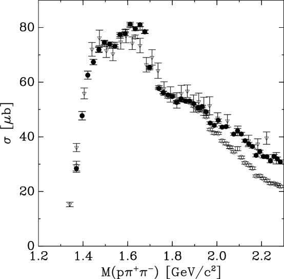
Figure 6: Results for the total cross section calculated from the partial wave analysis. Inverted triangles: Aachen-Berlin-Bonn-Hamburg-Heidelberg-München collaboration. Open circles: PWA using $s$-channel waves only. Filled Circles: PWA using $s$-channel waves and $t$-channel $\rho$ production.

as open circles. The points plotted as inverted triangles are from an earlier bubble chamber experiment at DESY [14]. The discrepancy above 1.9 GeV/c² is due to the fact that we are not using a sufficient set of waves to describe our data. It is easy to try including waves corresponding to $t$-channel production of $\rho$’s: gamp generates the amplitudes with a small change to the keyfile, and they can be included into the fit either coherently or incoherently. The result of such a fit, with an incoherent $t$-channel $\rho$ production wave is plotted in Fig. 6 as filled circles. We can see the agreement with the DESY experiment is much better, and the statistical errors, even of this partial data set, are much smaller.

We can verify the fit describes the data better by using the fitted production amplitudes and the calculated decay amplitudes to weight events (generated uniformly in phase space) that passed through the detector simulation. This gives us a Monte-Carlo data set distributed in the kinematic variables as the fit found. This Monte-Carlo data set can be compared to the real data to measure the quality of the fit and give clues about what waves need to be added. For example, Fig. 7

Figure 7: Comparison of $\cos(\theta_{cm})$ distributions of the proton for the data (solid circles), and the predictions of a fit using only $s$-channel waves (open squares), and a fit using $s$-channel waves with incoherent $t$-channel $\rho$ production (open circles).

shows the $\cos(\theta_{cm})$ distributions for the data (solid circles), and the Monte-Carlo “data” sets generated from the fits mentioned above: $s$-channel waves only and $s$-channel with incoherent $t$-channel $\rho$ production. These distributions are for $2.06662<M(p\pi^{+}\pi^{-})<2.08378$, where the total cross section is beginning to show discrepancy. The fit using only $s$-channel waves (open squares) cannot create an asymmetry large enough to describe the backward (in the center of mass system) proton peak; however adding a simple, incoherent $t$-channel $\rho$ production wave (open circle) improves the the description of this kinematic variable quite a bit.

5 Conclusions and Future Directions

The pwa2000 is a flexible suite of tools developed for partial wave analysis of particle physics data. It has been used to analyze peripheral meson production in a pion beam [15], peripheral meson production in a photon beam, and $s$-channel baryon resonance production in a photon beam [16]. The object defined in the library have been sufficient for all these analyses, the usual extent of the modification necessary are to the input file parser to handle input of information not required in previous analysis. For instance, the library implements the mass dependence of an isobar decay using an abstract base class massDep. As additional parameterizations are added for isobar decays, we add a derived class of massDep that implements the particular parameterization, add an appropriate keyword to the keyfile language and modify the yacc parser to instantiate the new derived class when it sees the new keyword.

The strategy of separating the intelligence of the program from the computation proved fruitful. By using a separate program to generate the input file for the fitting program, we were able to choose a language well suited to each particular task. prolog, a language known for its artificial intelligence applications, was used to apply the logical constraints to the likelihood function such as physical conservation laws. C++ routines were then driven by the input file prolog writes.

Our experiences with the pwa2000 have shown us possible avenues for future improvements. The large statistics that will be coming available from newer experiments will tremendously improve the statistical power of the results. Unfortunately this comes at a cost of speed: serial fits for a single mass bin of projected data volumes could take days. We have begun studies of parallelization of the maximum-likelihood fits. One approach is to utilize work being done on Grid Computing [17] or World-Wide Computing [18]. Such an approach may be fruitful for our problem since the evaluation of the likelihood function is almost trivially parallelizable being a large sum over $\approx 10^{6}-10^{8}$ events.

The authors wish to thank all those who suffered through buggy versions of this code. Their patience and suggestions have produced a robust system. This work was partially supported by the National Science Foundation.

References

- [1] S. Chung, Formulas for partial-wave analysis, note, BNL (1988).
- [2] S. Chung, T. Trueman, Positivity conditions on the spin density matrix: A simple parametrization, Physical Review D 11 (3) (1975) 633.
- [3] S. Chung, Spin formalisms, CERN Yellow Report 71-8, CERN (March 1971).
- [4] M. Jacob, G. C. Wick, On the general theory of collisions for particles with spin, Ann. Phys. 7 (1959) 404–428.
- [5] F. von Hippel, C. Quigg, Centrifugal-barrier effects in resonance partial decay widths, shapes, and production amplitudes, Physical Review D 5 (1972) 624.
- [6] S. Flatté, Coupled-channel analysis of the and systems near threshold, Physics Letters B 63 (1976) 224.
- [7] S. U. Chung, et al., Partial wave analysis in K matrix formalism, Annalen Phys. 4 (1995) 404–430.
- [8] N. Ramsey, Literate programming simplified, IEEE software 11(5) (1994) 97.
- [9] D. E. Knuth, Literate Programming, Center for the Study of Language and Information - Lecture Notes, University of Chicago Press, 1992.
- [10] K. L. Au, D. Morgan, M. R. Pennington, Meson dynamics beyond the quark model: Study of final-state interactions, Physical Review D 35 (1987) 1633.
- [11] D. V. Amelin, et al., Study of resonance production in diffractive reaction , Physics Letters B 356 (1995) 595.
- [12] S. U. Chung, et al., Exotic and resonances in the system produced in collisions at 18 GeV/, Phys. Rev. D65 (2002) 072001.
- [13] B. W. Kernighan, R. Pike, The UNIX programming environment, Prentice-Hall Software Series, Prentice-Hall, New Jersey, 1984.
- [14] ABBHHM, Photoproduction of meson and baryon resonances at energies up to 5.8-GeV, Phys. Rev. 175 (1968) 1669–1696.
- [15] M. Nozar, et al., A study of the reaction at 18-GeV/: The D and S decay amplitudes for , Phys. Lett. B541 (2002) 35–44.
- [16] M. Bellis, An analysis of using the CLAS detector, in: CIPANP-2003 proceedings, 2003.
- [17] I. Foster, C. Kesselman, Globus: A metacomputing infrastructure toolkit, The International Journal of Supercomputer Applications and High Performance Computing 11 (2) (1997) 115–128.
- [18] C. Varela, G. Agha, Programming dynamically reconfigurable open systems with SALSA, ACM SIGPLAN Notices 36 (12) (2001) 20–34.