Estimation of the linear transient growth of perturbations of cellular flames

Abstract

In this work we estimate rates of the linear transient growth of the perturbations of cellular flames governed by the Sivashinsky equation. The possibility and significance of such a growth was indicated earlier in both computational and analytical investigations. Numerical investigation of the norm of the resolvent of the linear operator associated with the Sivashinsky equation linearized in a neighbourhood of the steady coalescent pole solution was undertaken. The results are presented in the form of the pseudospectra and the lower bound of possible transient amplification. This amplification is strong enough to make the round-off errors visible in the numerical simulations in the form of small cusps appearing on the flame surface randomly in time. Performance of available numerical approaches was compared to each other and the results are checked versus directly calculated norms of the evolution operator.

Compiled on   at 2:14

Key words: nonnormal operator, pseudospectra, nonmodal amplification, hydrodynamic flame instability, cellular flames

PACS 2003: 47.70.Fw, 47.20.Ma, 47.20.Ky, 47.54.+r, 02.60.Nm

ACM computing classification system 1998: J.2, G.1.9, G.1.3, G.1.0

AMS subject classification 2000: 80A25, 76E15, 76E17, 35S10, 65G50

Abbreviated title: Transient growth of perturbations of cellular flames

1 Introduction

Sivashinsky’s equation

$$\frac{\partial\Phi}{\partial t}-\frac{1}{2}\left(\frac{\partial\Phi}{\partial x}\right)^{2}=\frac{\partial^{2}\Phi}{\partial x^{2}}+\frac{\gamma}{2}\frac{\partial{\cal H}[\Phi]}{\partial x},\qquad x\in\mbox{\boldmath${R}$},\qquad t>0,$$ (1)

governs evolution of the perturbation $\Phi(x,t)$ of the plane flame front moving in the direction orthogonal to the $x$-axis with the laminar flame speed $u_{b}$, see Fig. 1. Here space coordinates are measured in units of the flame front width $\delta_{th}$, time is in units of $\delta_{th}/u_{b}$, and ${\cal H}[\Phi]=\pi^{-1}\int\limits_{-\infty}^{\infty}(x-y)^{-1}\Phi(y,t)dy$ is the Hilbert transform.

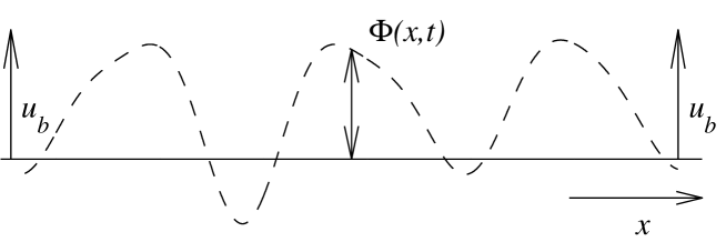
Figure 1: Perturbation (dashed line) of the plane flame front (solid line) moving at a speed $u_{b}$.

The equation was obtained in [1] considering the flame front as a surface separating combustible mixture of density $\rho_{u}$ and burnt gases of density $\rho_{b}$. Assumptions of the low expansion rate $\rho_{b}/\rho_{u}\approx 1$ and small flame surface gradient $|\nabla\Phi|\ll 1$ were also used in order to justify the appearance of the nonlinearity in (1), where the parameter $\gamma=1-\rho_{b}/\rho_{u}$.

A wide class of periodic solutions to (1) was obtained in [2] by using the pole decomposition technique. Namely, it was shown that

$$\Phi(x,t)=2\pi NL^{-1}\left(\gamma-4\pi NL^{-1}\right)t$$

$$+2\sum\limits_{n=1}^{N}\ln\left|\cosh\left[2\pi b_{n}(t)/L\right]-\cos\left\{2\pi[x-a_{n}(t)]/L\right\}\right|$$ (2)

is an $L$-periodic solution to (1) if

$$\frac{da_{n}}{dt}=-\frac{2\pi}{L}\sum\limits_{m=1}^{N}\left.\right.^{{}^{\prime}}\left\{\frac{\sin[2\pi(a_{n}-a_{m})/L]}{\cosh[2\pi(b_{n}-b_{m})/L]-\cos[2\pi(a_{n}-a_{m})/L]}\right.$$

$$+\left.\frac{\sin[2\pi(a_{n}-a_{m})/L]}{\cosh[2\pi(b_{n}+b_{m})/L]-\cos[2\pi(a_{n}-a_{m})/L]}\right\},$$ (3)

$$\frac{db_{n}}{dt}=2\pi L^{-1}\coth\left(2\pi b_{n}/L\right)-(\gamma/2)\mbox{sign}b_{n}$$

$$+\frac{2\pi}{L}\sum\limits_{m=1}^{N}\left.\right.^{{}^{\prime}}\left\{\frac{\sinh[2\pi(b_{n}-b_{m})/L]}{\cosh[2\pi(b_{n}-b_{m})/L]-\cos[2\pi(a_{n}-a_{m})/L]}\right.$$

$$+\left.\frac{\sinh[2\pi(b_{n}+b_{m})/L]}{\cosh[2\pi(b_{n}+b_{m})/L]-\cos[2\pi(a_{n}-a_{m})/L]}\right\}.$$ (4)

Here $N$ is an arbitrary positive integer and prime in the symbol of summation means $m\neq n$. Pairs of real numbers $(a_{n},b_{n})$, $n=1,\ldots,N$ are called poles and, correspondingly, function (2) is called $N$-pole solution to (1). It is also convenient to consider $\Phi(x,t)\equiv{\rm const}$ as a $0$-pole solution to (1).

If all the poles in (3), (4) are steady and $a_{n}=a\in\mbox{\boldmath${R}$}$ for $n=1,\ldots,N$, then, (2) is called a steady coalescent $N$-pole solution. Solutions of the latter type, denoted here as $\Phi_{N}(x)$ and illustrated in Fig. 2, have been found to be the strongest attractors of (1) and the period $L$ preferred by (1) has appeared to coincide with the size of the whole computational domain which we therefore denote as $[-L/2,L/2]$, see e.g. [3].

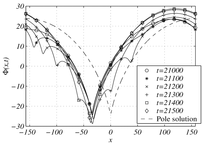
Figure 2: Steady coalescent $N$-pole solutions to the Sivashinsky equation. Here $\gamma=0.8$ and $L=100\pi$ ($N_{L}=10$). Graphs have been shifted vertically in order to get $\Phi_{N}(\pm L/2)=0$.

It was shown, see for example [4], that for a given period $L$ the number of poles in steady coalescent pole solution (2) may not exceed $N_{L}={\rm ceil}(\gamma L/8\pi+1/2)-1$, where ${\rm ceil}(x)$ is the smallest integer greater or equal to $x$. Direct numerical simulations have revealed, in turn, that for sufficiently small values of $L<L_{c}$ the preferred number of poles is equal $N_{L}$. This observation was explained in [5] by means of the eigenvalue analysis of (1) linearized in a neighbourhood of the steady coalescent pole solutions. The analysis has indicated that for any $L>0$ the steady coalescent $N_{L}$-pole solution is the only steady coalescent $N$-pole solution to (1) with all the eigenvalues located in the left half of the complex plane. Strictly speaking, [5] does not provide a solid proof that their set of eigenvalues is complete and in this paper we explain why the comparison with the direct numerical calculation of the spectra, used in [5], cannot justify the completeness, in particular for large enough $L$.

Surprisingly, for larger computational domains $L>L_{c}$, numerical solutions to (1) do not stabilize to any steady coalescent $N$-pole solution at all. Instead, being essentially nonsteady, they remain very closely to the steady coalescent $N_{L}$-pole solution, developing on the surface of the flame front small cusps randomly in time, see e.g. [6]. With time these small cusps move towards the trough of the flame front profile and disappear in it as this is shown in Fig. 2.

The high sensitivity of pole solutions to certain perturbations was suggested in [7] as an explanation of the cardinal change in the behaviour of numerical solutions to (1) which takes place for $L=L_{c}$. The argument of [7] was based on a particular asymptotic solution to an approximation of the Sivashinsky equation linearized in a neighbourhood of the steady coalescent $N$-pole solution. In the following works, see e.g. [8], the approach has been developed further and a model equation with stochastic right hand side, explicitly representing the noise, has been proposed and investigated. Sensitivity of Sivashinsky equation to the noise has also been studied in [9], and an estimation of dependence between $L_{c}$ and the amplitude of noise in the form of the the round-off errors has been obtained in [6] in a series of direct numerical simulations.

Similar insufficiency of the eigenvalue analysis to interpret time dependent behaviour of asymptotically stable systems is also known from problems of classic hydrodynamics, such as Poiseuille and Hagen-Poiseuille flows [10]. The failure of the spectral analysis in these problems was linked to the nonorthogonality of the eigenfunctions of the associated linearized operators and was explained by the estimation of possible transient growth of perturbations [11], [12]. A convenient tool to estimate possible transient growth of solutions governed by nonnormal operators were developed during the last decade in the form of the pseudospectra [13]. Corresponding numerical techniques have been reviewed in [14].

In this work we estimate rates of the linear transient growth of the perturbations of the steady coalescent $N_{L}$-pole solutions to the Sivashinsky equation. In Section 2 we linearize the equation in a neighbourhood of the steady coalescent pole solution. In Section 3, results of direct computations of the pseudospectra of the linear operator are presented. Also, a comparison of performance of available numerical techniques is given. Estimation of the rates of growth in terms of Kreiss constants, norms of the $C_{0}$-semigroup and condition numbers, are presented in Section 4. We conclude with a discussion and a summary of results in Section 5.

2 Linearized Sivashinsky equation

Substituting $\Phi(x,t)=\Phi_{N}(x,t)+\phi(x,t)$ into (1) and neglecting terms which are nonlinear in $\phi(x,t)$, one obtains

$$\frac{d\phi}{dt}={\cal A}_{N}\phi,\qquad t>0,$$ (5)

where operator ${\cal A}_{N}$ is defind by the following integro-differential expression

$${\cal A}_{N}u=\Psi_{N}\frac{\partial u}{\partial x}+\frac{\partial^{2}u}{\partial x^{2}}+\frac{\gamma}{2}\frac{\partial{\cal H}[u]}{\partial x},\qquad x\in\mbox{\boldmath${R}$},$$ (6)

on sufficiently smooth $L$-periodic functions with the square integrable on $[-L/2,L/2]$. Here

$$\Psi_{N}=\frac{\partial\Phi_{N}}{\partial x}=\frac{4\pi}{L}\sum\limits_{n=1}^{N}\frac{\sin[2\pi(x-a)/L]}{\cosh(2\pi b_{n}/L)-\cos[2\pi(x-a)/L]},$$ (7)

$L>0$ and $a\in\mbox{\boldmath${R}$}$ are real parameters, and the set $b_{n}$, $n=1,\ldots,N$ is the steady solution to (4).

The adjoint integro-differential expression is

$${\cal A}_{N}^{*}u=-\frac{\partial\Psi_{N}u}{\partial x}+\frac{\partial^{2}u}{\partial x^{2}}+\frac{\gamma}{2}\frac{\partial{\cal H}[u]}{\partial x},\qquad x\in\mbox{\boldmath${R}$}.$$ (8)

Hence, ${\cal A}_{N}{\cal A}_{N}^{*}$ $\neq{\cal A}_{N}^{*}{\cal A}_{N}$ for $N>0$, and operator ${\cal A}_{N}$ is nonnormal. However, for $0$-pole solution the first term in the right hand side of (6) disappears and operator ${\cal A}_{N}$ is normal. In this sense we can say that it is the nonlinearity of the Sivashinsky equation what makes its associated linearized operator ${\cal A}_{N}$ nonnormal.

If (5), (6) is differentiated by $x$, then the resulting equation for $\psi(x)=d\phi/dx$ is $\partial\psi/\partial t={\cal A^{\prime}}_{N}\psi$, where

$${\cal A^{\prime}}_{N}\psi=\frac{\partial\Psi_{N}\psi}{\partial x}+\frac{\partial^{2}\psi}{\partial x^{2}}+\frac{\gamma}{2}\frac{\partial{\cal H}[\psi]}{\partial x},\qquad x\in\mbox{\boldmath${R}$}.$$

The eigenvalue problem ${\cal A^{\prime}}_{N}v=\lambda v$ was studied in [5]. Obviously, eigenvalues of ${\cal A}_{N}$ and ${\cal A^{\prime}}_{N}$ are the same and the eigenfunctions of the latter one are just $x$-derivatives of the eigenfunctions of the operator ${\cal A}_{N}$.

In accordance with [5], operator ${\cal A^{\prime}}_{N}$ has a zero eigenvalue associated with the $x$-shift invariance of (1). The same is true for ${\cal A}_{N}$ as well. Moreover, zero is at least a double eigenvalue of ${\cal A}_{N}$, because (1) is also $\Phi$-shift invariant. Here, $x$- and $\Phi$-shift invariance means, that if $\Phi(x,t)$ is a solution to (1), then, for any $C_{1},C_{2}\in\mbox{\boldmath${R}$}$, function $\Phi(x+C_{1},t)+C_{2}$ is its solution either.

If only solutions with the period $L$ are of interest, then they can be represented by the Fourier series $\phi(x,t)=\sum\limits_{k=-\infty}^{\infty}\widetilde{\phi}_{k}e^{i2\pi kx/L}$. Substituting these series into (5), (6) multiplying the result by $e^{i2\pi nx/L}$, and integrating over the interval $x\in[-L/2,L/2]$, we obtain

$$\frac{d\widetilde{\phi}_{k}}{dt}=\left(-\frac{4\pi^{2}}{L^{2}}k^{2}+\frac{\pi\gamma}{L}|k|\right)\widetilde{\phi}_{k}(t)+i\frac{2\pi}{L}\sum\limits_{m=-\infty}^{\infty}m\widetilde{\Psi_{N}}(k-m)\widetilde{\phi}_{m}(t),$$ (9)

where $\widetilde{\Psi_{N}}(k)=L^{-1}\int_{-L/2}^{L/2}\Psi_{N}(x)e^{-i2\pi kx/L}dx$ and $|k|<\infty$. The integral can be written as a linear combination of the integrals of type $\int_{0}^{\pi}\cos my\ (\alpha-\cos y)^{-1}dy$ and the latter one was evaluated by using entry 2.5.16.33, p. 415 of [15] yielding

$$\widetilde{\Psi_{N}}(k)=-i4\pi L^{-1}\mbox{sign}(k)e^{-i2\pi ka/L}\sum\limits_{n=1}^{N}e^{-2\pi b_{n}|k|/L},$$ (10)

Introducing the representation of (5) in the Fourier space $d\widetilde{\phi}/dt=\widetilde{{\cal A}_{N}}\widetilde{\phi}$, the Fourier image $\widetilde{{\cal A}_{N}}$ of the operator ${\cal A}_{N}$ is defined by the $(k,m)$-th entry of its double infinite ($-\infty<k,m<\infty$) matrix as follows

$$(\widetilde{{\cal A}_{N}})_{k,m}=\left(-4\pi^{2}L^{-2}k^{2}+\pi\gamma L^{-1}|k|\right)\delta_{k,m}$$

$$+8\pi^{2}L^{-2}m\mbox{sign}(k-m)e^{-i2\pi(k-m)a/L}\sum\limits_{n=1}^{N}e^{-2\pi b_{n}|k-m|/L},\qquad|k|,|m|<\infty,$$ (11)

where $\delta_{k,m}$ is the Kronecker’s symbol.

It can be shown, that the value of the free parameter $a$ does not affect neither spectral properties of $\widetilde{{\cal A}_{N}}$ nor its $2$-norms. Hence, we consider the case $a=0$ only.

3 Pseudospectra of the linear operator

3.1 Computational techniques

In what follows we will work with matrix (11) cut off at $|k|,|m|=K$, i.e. all $(k,m)$ entries of $\widetilde{{\cal A}_{N}}$ with either $|k|$ or $|m|$ greater than $K$ are neglected. Thus, instead of matrix $\widetilde{{\cal A}_{N}}$ acting on double infinite vectors $\widetilde{\phi}$, we consider the $(2K+1)\times(2K+1)$ matrix $\widetilde{{\cal A}_{N}^{(K)}}$, whose entries coincide with those of $\widetilde{{\cal A}_{N}}$ for $-K\leq k,n\leq K$.

In accordance with [14], in order to estimate possible nonmodal amplification of solutions in (5), we first calculate values of $\left\|\left(z{\cal I}-\widetilde{{\cal A}_{N}}^{(K)}\right)^{-1}\right\|_{2}$ as a function of the complex parameter $z$ for large enough values of $K$. Level lines of this function form boundaries of the pseudospectra of $\widetilde{{\cal A}_{N}}^{(K)}$, see [13]. It was found in numerical experiments that a good level of accuracy of the most interesting part of the pseudospectra of $\widetilde{{\cal A}_{N}}$ is achieved if the cut off parameter $K$ is about $2L/\pi$ or greater. Thus, and in virtue of the Parseval identity $\left\|(z{\cal I}-{\cal A}_{N})^{-1}\right\|_{{\cal L}_{2}}$ $=\left\|\left({z\cal I}-\widetilde{{\cal A}_{N}}\right)^{-1}\right\|_{2}$ , speaking about pseudospectra or other ${\cal L}_{2}$-norm based functionals of ${\cal A}_{N}$ we actually mean those calculated for $\widetilde{{\cal A}_{N}}^{(K)}$ with large enough $K$. Here and in what follows $\cal I$ is the unity operator or matrix of an appropriate size.

Calculations of $\left\|\left(z{\cal I}-\widetilde{{\cal A}_{N}}^{(K)}\right)^{-1}\right\|_{2}$ can be carried out straightforwardly, however computational costs can be reduced if $\widetilde{{\cal A}_{N}}^{(K)}$ is transformed appropriately. By construction, matrix $\widetilde{{\cal A}_{N}}^{(K)}$ acts on vectors $\widetilde{u}^{(K)}$ $=(\widetilde{u}_{-K},\ldots,\widetilde{u}_{-1},$ $\widetilde{u}_{0},$ $\widetilde{u}_{1},\ldots,\widetilde{u}_{K})^{\top}$. Let us rearrange their components and consider $\widetilde{w}^{(K)}$ $=\left[\widetilde{u}_{0},\right.$ $\left(\widetilde{u}^{(K)}_{-}\right)^{\top},$ $\left.\left(\widetilde{u}^{(K)}_{+}\right)^{\top}\right]^{\top}$, where $\widetilde{u}^{(K)}_{\pm}$ $=(\widetilde{u}_{\pm 1},\ldots,\widetilde{u}_{\pm K})^{\top}$. The permutation matrix $\cal P$, corresponding to the proposed rearrangement $\widetilde{w}^{(K)}={\cal P}\widetilde{u}^{(K)}$, transforms $\widetilde{{\cal A}_{N}}^{(K)}$ into ${\cal P}\widetilde{{\cal A}_{N}}^{(K)}{\cal P}^{-1}$, which acts on $\widetilde{w}^{(K)}$ and has the following structure

$${\cal P}\widetilde{{\cal A}_{N}}^{(K)}{\cal P}^{-1}=\left(\begin{array}[]{rrr}0&{\cal C}&{\cal C}\\ 0&{\cal D}+{\cal A}^{(1)}&{\cal A}^{(2)}\\ 0&{\cal A}^{(2)}&{\cal D}+{\cal A}^{(1)}\\ \end{array}\right).$$ (12)

One zero eigenvalue of $\widetilde{{\cal A}_{N}}^{(K)}$, corresponding to the $\Phi$-shift invariance of (1), can be seen from (12) explicitly. For other blocks of (12) we have:

$$\begin{array}[]{lll}{\cal C}_{m}&=-8\pi^{2}L^{-2}|m|\sum\limits_{n=1}^{N}e^{-2\pi b_{n}|m|/L},&m=1,2,\ldots,K,\end{array}$$

$$\begin{array}[]{lll}{\cal D}_{k,m}&=\left(-4\pi^{2}L^{-2}k^{2}+\pi\gamma L^{-1}|k|\right)\delta_{k,m},&k,m=1,2,\ldots,K,\\ &&\\ {\cal A}^{(1)}_{k,m}&=8\pi^{2}L^{-2}m\mbox{sign}(k-m)\sum\limits_{n=1}^{N}e^{-2\pi b_{n}|k-m|/L},&k,m=1,2,\ldots,K,\\ &&\\ {\cal A}^{(2)}_{k,m}&=-8\pi^{2}L^{-2}m\mbox{sign}(k+m)\sum\limits_{n=1}^{N}e^{-2\pi b_{n}|k+m|/L},&k,m=1,2,\ldots,K.\end{array}$$

Following the idea of [5], we apply the similarity transform

$${\cal T}=\frac{1}{\sqrt{2}}\left(\begin{array}[]{rrr}1&0&0\\ 0&{\cal I}&{\cal I}\\ 0&{\cal I}&-{\cal I}\\ \end{array}\right)$$

to ${\cal P}\widetilde{{\cal A}_{N}}^{(K)}{\cal P}^{-1}$. Here $\cal I$ is the unity $K\times K$ matrix corresponding to the block structure of (12). Unlike [5], the normalizing coefficient $1/\sqrt{2}$ was chosen to preserve the $2$-norm. The transformed matrix ${\cal T}{\cal P}\widetilde{{\cal A}_{N}}^{(K)}({\cal T}{\cal P})^{-1}$ is decoupled into two diagonal blocks

$${\cal T}{\cal P}\widetilde{{\cal A}_{N}}^{(K)}({\cal T}{\cal P})^{-1}=2\left(\begin{array}[]{rrr}0&{\cal C}&0\\ 0&{\cal D}+{\cal A}^{(1)}+{\cal A}^{(2)}&0\\ 0&0&{\cal D}+{\cal A}^{(1)}-{\cal A}^{(2)}\\ \end{array}\right),$$ (13)

and has the same $2$-norm as $\widetilde{{\cal A}_{N}}^{(K)}$. The $2$-norm of (13) is the maximum of 2-norms of its two blocks, each of which is of twice smaller size than ${\cal T}{\cal P}\widetilde{{\cal A}_{N}}^{(K)}({\cal T}{\cal P})^{-1}$. In practice, the number of arithmetic operations required to estimate the $2$-norm of a matrix is of the order of the cube of its size. Therefore, estimation of the $2$-norm of $\widetilde{{\cal A}_{N}}^{(K)}$ through blocks of ${\cal T}{\cal P}\widetilde{{\cal A}_{N}}^{(K)}({\cal T}{\cal P})^{-1}$ is more efficient. From our experience, the $2$-norms of the blocks are of the same order of magnitude, although the $2$-norm of the upper block supersedes the lower one for most of practically important values of $z$.

A straightforward and reliable way to calculate the $2$-norm of the resolvent of $\widetilde{{\cal A}_{N}}^{(K)}$ (or of diagonal blocks of (13)) is through the singular value decomposition (SVD). Namely, the reciprocal to the smallest singular value $s_{0}$ of $z{\cal I}-\widetilde{{\cal A}_{N}}^{(K)}$ is equal to $\left\|\left(z{\cal I}-\widetilde{{\cal A}_{N}}^{(K)}\right)^{-1}\right\|_{2}$, see [14]. The direct Matlab implementation of SVD worked well in our case, though a few inverse iterations with continuation in $z$, suggested in [16], appeared to be as accurate and, on average, about six times faster.

An alternative algorithm is based on projection to the interesting subspace through the Schur factorization followed by the Lanczos iterations. It was suggested in [14] in the form of a Matlab script and is, on average, about two times faster than inverse iterations with continuation. Further, our tests have shown that its efficiency degrades much slower as the matrix size or required accuracy grows. Thus, Schur factorization with Lanczos iterations was the algorithm of our choice. It was intensively monitored by the direct SVD, however.

A comparison of performance of the inverse iterations with continuation and of the Schur factorization with Lanczos iterations is given in Fig. 3 for calculations of $\left\|\left(z{\cal I}-\widetilde{{\cal A}_{N}}^{(K)}\right)^{-1}\right\|_{2}$ with $L=40\pi$, $\gamma=0.8$ and $K=80$. The criteria of stopping the iterations was $\left|s_{0}^{(n)}-s_{0}^{(n-1)}\right|/s_{0}^{(n)}<0.01$, i.e. when the relative increment of the $n$-th approximation $s_{0}^{(n)}$ to the smallest singular value $s_{0}$ of $z{\cal I}-\widetilde{{\cal A}_{N}}^{(K)}$ is smaller than $\varepsilon=0.01$. Graphs reveal areas with slower convergence of iterations. Unlike the number of required inverse iterations is usually less than the number of the Lanczos ones, the latter are much cheaper computationally, resulting in a significantly better overall performance.

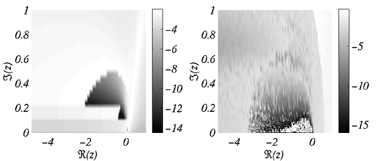
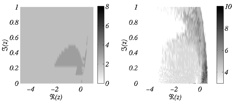
Figure 3: Relative increment of the smallest singular value in the last iteration (top) and number of iterations (bottom) carried out by methods [16] (left) and [14] (right).

3.2 Structure of the pseudospectra

As we are interested in stability of the steady coalescent pole solutions and possible rate of linear growth of their perturbations, the vicinity of the imaginary axis is of principle interest. Reflection symmetry of the function $\left\|\left(z{\cal I}-{\cal A}_{N}\right)^{-1}\right\|_{2}$ in regard to the real axis proves it sufficient, for our purposes, to study it in the region $z\in\{z:-5<\Re(z)<1,\ 0<\Im(z)<1\}$ only.

Figures 4a and 4b illustrate level lines of $\left\|\left(z{\cal I}-{\cal A}_{N}\right)^{-1}\right\|_{2}$ for $L=40\pi$ and $\gamma=0.8$. A rectangle plotted with a dashed line in Fig. 4a marks the location of the area magnified in Fig. 4b. Asterisks in the figures show approximations to the eigenvalues of the operator ${\cal A}_{N}$. These parameters correspond to the appearance of microcusps in our direct numerical simulations with single accuracy. The picture suggests that the large area of high values of $\left\|\left(z{\cal I}-{\cal A}_{N}\right)^{-1}\right\|_{2}$ near the origin can be the reason of significant amplification of the round-off errors, which in the case of single accuracy are of order $10^{-7}$.

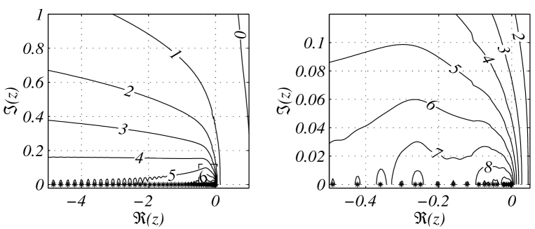
(a)                                                            (b)

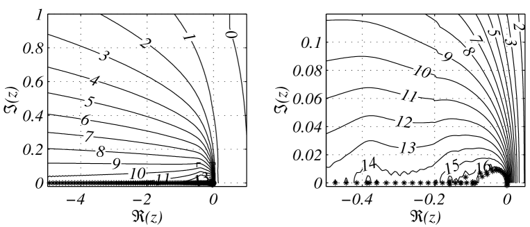
(c)                                                            (d)

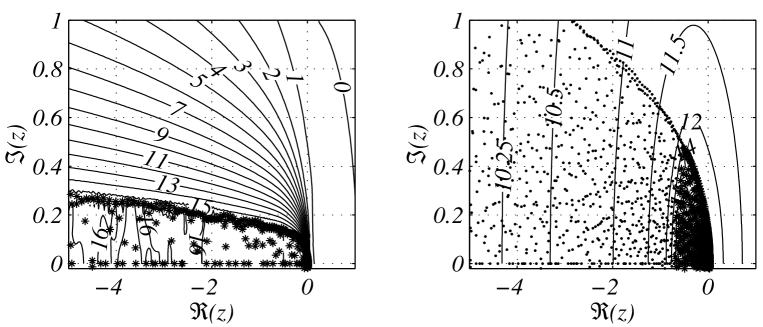
(e)                                                            (f)

Figure 4: Level lines of $\log_{10}\left\|\left(z{\cal I}-{\cal A}_{N}\right)^{-1}\right\|_{2}$ for $\gamma=0.8$. $L=40\pi$, $K=80$ in (a), (b); $L=90\pi$, $K=180$ in (c), (d); $L=200\pi$, $K=400$ in (e); $L=1000\pi$, $K=2000$ in (f).

Second critical case corresponding to the appearance of microcusps in calculations with double accuracy, see Fig. 2, is shown in Figs. 4c and 4d. Again, a large region of huge values of $\left\|\left(z{\cal I}-{\cal A}_{N}\right)^{-1}\right\|_{2}$ near $z=0$ suggests a possible match with the magnitude of the round-off errors which are of order $10^{-16}$ in this case.

Data on the $2$-norm of the resolvent of ${\cal A}_{N}$ for $L=200\pi$ and $\gamma=0.8$ are given in Fig. 4e. The figure shows further widening of the area of large values of $\left\|\left(z{\cal I}-{\cal A}_{N}\right)^{-1}\right\|_{2}$ near the real axis. Accordingly, calculated eigenvalues spread further from the real axis and to the right from the imaginary axis. Also, they tend to form a cluster near the level line $\left\|\left(z{\cal I}-{\cal A}_{N}\right)^{-1}\right\|_{2}$ $=10^{15}$, cf [14].

Also, Fig. 4e demonstrates that our calculations fail to produce reliable results if the smallest singular value $s_{0}$ of $z{\cal I}-\widetilde{{\cal A}_{N}}^{(K)}$ is less than about $10^{-15}$. This is because of the effect of the round-off errors of the computer on the computational algorithm used to estimate $s_{0}$. We see, however, that level lines of $\left\|\left(z{\cal I}-{\cal A}_{N}\right)^{-1}\right\|_{2}$ corresponding to $s_{0}\geq 10^{-15}$ are much less sensitive to these round-off errors than the eigenvalues.

All the algorithms for estimation of pseudospectra mentioned in Section 3.1 are subject to the effect of the round-off errors and special arrangements are required in order to get reliable results for $s_{0}<10^{-15}$. In particular, calculations with 128-bit arithmetic, implemented in some computer systems, can be used. However, for our purposes knowledge of $\left\|\left(z{\cal I}-{\cal A}_{N}\right)^{-1}\right\|_{2}$ corresponding to $s_{0}\geq 10^{-15}$ is sufficient.

The last example of the pseudospectra for $L=1000\pi$ shown in Fig. 4f was calculated in a different way. The matrix $\widetilde{{\cal A}_{N}}^{(K)}$ for $K=2000$ was projected into its eigenspace spanning 1000 eigenvectors corresponding to the eigenvalues with the smallest absolute values. Then, the projected matrix was used to estimate the level lines of $\left\|\left(z{\cal I}-{\cal A}_{N}\right)^{-1}\right\|_{2}$ depicted in Fig. 4f. The eigenvalues used for the projection are denoted by asterisks, the neglected ones by dots. The eigenvalue problem for the original matrix of size $4001\times 4001$ was solved by the Matlab implementation of $QR$-iterations. We also tried to apply Arnoldi iterations in accordance with [17], but could not make them convergent even for the projection subspaces of smaller dimensions and for smaller values of $L$.

The direct calculation of the approximation to the spectrum of ${\cal A}_{N}$, namely eigenvalues of $\widetilde{{\cal A}_{N}}^{(K)}$ presented in Figs. 4a - 4f with asterisks and dots, was undertaken by the Matlab implementation of $QR$-iterations. In the case of $L=90\pi$ six directly calculated eigenvalues are located to the right from the imaginary axis, see also [9]. The number of eigenvalues in the right half of the complex plane grows for larger $L$. However, the pseudospectra plotted in Figs. 4d - 4f suggest that these unstable eigenvalues cannot be trusted. They appear in the vast area of large values of $\left\|\left(z{\cal I}-{\cal A}_{N}\right)^{-1}\right\|_{2}$ and, in accordance with e.g. [13], can be very sensitive to the perturbations as small as $10^{-16}$, which is on the level of the machine zero in the case in question.

Every eigenvalue $\lambda$ of $\widetilde{{\cal A}_{N}}^{(K)}$ can be associated with a condition number $\kappa_{\lambda}$ $=|\sum_{i}w_{i}u_{i}|^{-1}$, where $w$ and $u$ are corresponding normalized left and right eigenvectors of $\widetilde{{\cal A}_{N}}^{(K)}$, see [18]. Then, eigenvalues of $\widetilde{{\cal A}_{N}}^{(K)}$ will be perturbed by $\kappa_{\lambda}\|{\cal E}\|_{2}$ at most, if $\widetilde{{\cal A}_{N}}^{(K)}$ is perturbed by matrix $\cal E$ with small enough $\|{\cal E}\|_{2}$. Figure 5 illustrates these condition numbers for $L=40\pi$ and $90\pi$, making a very good match to the magnitude of perturbations of eigenvalues given in Fig. 4d. Note, the rightmost eigenvalues are worst conditioned.

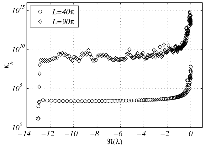
Figure 5: Condition numbers of the eigenvalues $\lambda$ of $\widetilde{{\cal A}_{N}}^{(K)}$ for $\gamma=0.8$.

We would like to stress that because of the severe nonnormality of $\widetilde{{\cal A}_{N}}^{(K)}$ some of its directly calculated eigenvalues may have nothing in common with what they should be in absence of the round-off errors. A particular numerical method can even worsen the estimation indeed. However, no one method can reduce the perturbation associated with the approximation of entries of $\widetilde{{\cal A}_{N}}^{(K)}$ by the finite-digit arithmetic of the computer, cf [5]. The only way to increase the accuracy of the direct eigenvalue computations for $L\geq 90\pi$ is to use a more accurate computer arithmetic with machine zero smaller than the reciprocal of $\max\limits_{\lambda\in\Lambda(\widetilde{{\cal A}_{N}}^{(K)})}\{\kappa_{\lambda}\}$, where $\Lambda(\widetilde{{\cal A}_{N}}^{(K)})$ is the spectrum of $\widetilde{{\cal A}_{N}}^{(K)}$.

4 Estimation of the transient amplification

4.1 Kreiss constants

A robust lower bound on $\left\|e^{t{\cal A}_{N}}\right\|_{{\cal L}_{2}}$ can be obtained from the Laplace transform of $e^{t{\cal A}_{N}}$, which under certain conditions (see [19]) can be written as

$$\int\limits_{0}^{\infty}e^{-zt}e^{t{\cal A}_{N}}dt=(z{\cal I}-{\cal A}_{N})^{-1}.$$

Considering norms of both sides of this relation and carrying out straightforward estimations of the integral:

$$\|(z{\cal I}-{\cal A}_{N})^{-1}\|_{{\cal L}_{2}}=\left\|\int\limits_{0}^{\infty}e^{-zt}e^{t{\cal A}_{N}}dt\right\|_{{\cal L}_{2}}\leq\sup\limits_{t>0}\|e^{t{\cal A}_{N}}\|_{{\cal L}_{2}}\int\limits_{0}^{\infty}e^{-\Re(z)t}dt,$$

we arrive at $\sup\limits_{t>0}\|e^{t{\cal A}_{N}}\|_{{\cal L}_{2}}\geq\Re(z)\|(z{\cal I}-{\cal A}_{N})^{-1}\|_{{\cal L}_{2}}$. The latter is valid for all $z$ with positive real part yielding

$$\sup\limits_{t>0}\|e^{t{\cal A}_{N}}\|_{{\cal L}_{2}}\geq\sup\limits_{\Re(z)>0}\left[\Re(z)\|(z{\cal I}-{\cal A}_{N})^{-1}\|_{{\cal L}_{2}}\right]={\cal K}_{{\cal A}_{N}},$$ (14)

where ${\cal K}_{{\cal A}_{N}}$ is called the Kreiss constant, see also [12], [13]. In other words, if ${\cal K}_{{\cal A}_{N}}$ is the Kreiss constant of the operator ${\cal A}_{N}$, then there is a perturbation $\phi_{*}(x,t)$ governed by (5) and a time instance $t_{*}$ such that the initial value of $\phi_{*}(x,t)$ is amplified at least ${\cal K}_{{\cal A}_{N}}$ times in terms of its ${\cal L}_{2}$ norm, i.e. $\|\phi_{*}(x,t_{*})\|_{{\cal L}_{2}}$ $\geq{\cal K}_{{\cal A}_{N}}\|\phi_{*}(x,0)\|_{{\cal L}_{2}}$.

Our studies of pseudospectra represented, in particular, in Figs. 4a - 4f indicate that the supremum in (14) is reached on the real axis. Figure 6 shows dependence of the function $z\left\|\left({\cal I}-z\widetilde{{\cal A}_{N}}^{(K)}\right)^{-1}\right\|_{2}$ on $z$ for $\Im(z)=0$. We depicted results obtained by three different techniques and they are in good agreement with each other except for very small $z$. The discrepancy for $z\leq 10^{-9}$ is because of the round-off errors as explained in the previous section. The smallest singular value $s_{0}$ of ${\cal I}-z\widetilde{{\cal A}_{N}}^{(K)}$ should be of order $10^{-15}$ to result in $z\left\|\left({\cal I}-z\widetilde{{\cal A}_{N}}^{(K)}\right)^{-1}\right\|_{2}$ $\approx 10^{6}$ for $z\approx 10^{-9}$. Indeed, this value of $s_{0}$ is too small to be accurately calculated on a computer with machine zero of order $10^{-16}$. It is quite reliable to conclude in this case that ${\cal K}_{{\cal A}_{N}}\geq 1.6\times 10^{6}$ for $L=40\pi$ and $\gamma=0.8$.

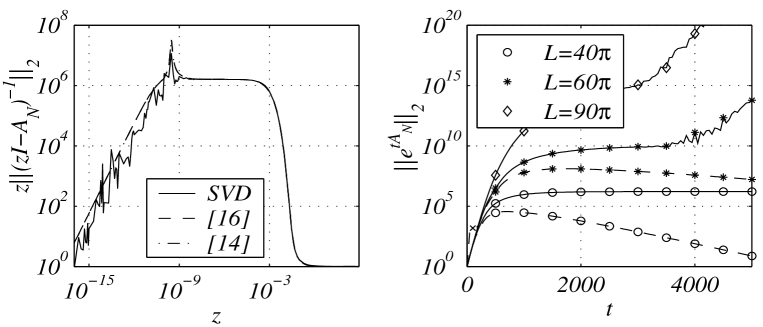
Figure 6: An approximation to $z\left\|\left(z{\cal I}-{\cal A}_{N}\right)^{-1}\right\|_{2}$ versus $z$ on the real axis for $L=40\pi$ and $K=160$ (left). Dependence of ${\cal L}_{2}$ norms of $C_{0}$-semigroups generated by $\widetilde{{\cal A}_{N}}^{(K)}$ (solid lines) and $\widetilde{{\cal B}_{N}}^{(K)}$ (dashed lines) on $t$ (right). Here $\gamma=0.8$.

Because of the effect of the round-off errors on the computation of $s_{0}$, similar estimations of the Kreiss constant for $L\geq 80\pi$ on a computer with the machine zero of order $10^{-16}$ are not accurate yielding a saturated value of order $10^{13}$. Instead, we have calculated more values of the Kreiss constant for a set of smaller $L$. Results are presented in Table 1 and Fig. 9.

Table 1: Estimated Kreiss constants of ${\cal A}_{N_{L}}$

$L/\pi$ $10$ $20$ $30$ $40$ $50$ ${\cal K}_{{\cal A}_{N}}$ $7.0\times 10^{0}$ $3.3\times 10^{2}$ $2.1\times 10^{4}$ $1.6\times 10^{6}$ $1.3\times 10^{8}$ $L/\pi$ $60$ $70$ $80$ $90$ $100$ ${\cal K}_{{\cal A}_{N}}$ $1.2\times 10^{10}$ $4.0\times 10^{11}$ $5.0\times 10^{12}$ $1.5\times 10^{13}$ $1.5\times 10^{13}$

4.2 Norms of the $C_{0}$-semigroup

Good supplementary proof of essential nonmodal amplification can be provided by direct estimation of the ${\cal L}_{2}$ norm of the $C_{0}$-semigroup generated by ${\cal A}_{N}$. Similar to the previous estimations, we have calculated the $2$-norm of the $C_{0}$-semigroup generated by $\widetilde{{\cal A}_{N}}^{(K)}$. Matlab’s implementation of a scaling and squaring algorithm with a Padé approximation has been used in order to avoid calculation of the Jordan decomposition of $\widetilde{{\cal A}_{N}}^{(K)}$. The results revealed a good convergence for $K\geq 2L/\pi$.

As we have mentioned in Section 2, operator ${\cal A}_{N}$ has a nontrivial null-space ${\cal N}({\cal A}_{N})$. Because of this $\left\|e^{t{\cal A}_{N}}\right\|_{{\cal L}_{2}}$ does not decay for $t\rightarrow\infty$ and, moreover, it grows slowly because of the round-off errors. In order to remove the effect of the null-space on the asymptotics of decay, and also, to demonstrate that the amplification observed in numerical experiments was not caused by that double zero eigenvalue, associated with the translational modes, we have projected $\widetilde{{\cal A}_{N}}^{(K)}$ into its eigenspace ${\cal N}\left(\widetilde{{\cal A}_{N}}^{(K)}\right)^{\perp}$ orthogonal to ${\cal N}\left(\widetilde{{\cal A}_{N}}^{(K)}\right)$. The 2-norms of the $C_{0}$-semigroups generated by the resulting operator, denoted here as $\widetilde{{\cal B}_{N}}^{(K)}$, are depicted in Fig. 6b alongside with the similar data for the original operator $\widetilde{{\cal A}_{N}}^{(K)}$.

Construction of $\widetilde{{\cal B}_{N}}^{(K)}$ for larger values of $L$ is complicated by difficulties with the accurate identification of the eigenfunctions corresponding to the zero eigenvalues. The latter ones appear to be perturbed and are as distant from $z=0$ as a few other eigenvalues. Note, that projection of $\widetilde{{\cal A}_{N}}^{(K)}$ into ${\cal N}\left(\widetilde{{\cal A}_{N}}^{(K)}\right)^{\perp}$ affects the $C_{0}$-semigroup not only asymptotically for $t\rightarrow\infty$, but for $t\rightarrow 0$ as well.

Data in Fig. 6b matches our estimations of the lower bound of the possible amplification of perturbations to the Sivashinsky equation and their extrapolations for larger values of $L$. Also, they show that presence of the nontrivial null space, corresponding to the shift invariance of the equation is not responsible for high sensitivity of the steady coalescent pole solutions to the noise. The latter conclusion is reinforced by the comparison of the pseudospectra of $\widetilde{{\cal A}_{N}}^{(K)}$ and $\widetilde{{\cal B}_{N}}^{(K)}$. On scales of Figs. 4a and 4b they are simply indistinguishable and can only be seen in a very close proximity of the origin, as shown in Fig. 7.

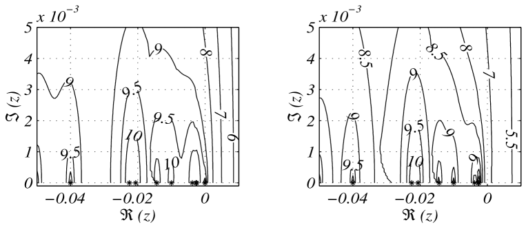
Figure 7: Comparison of level lines of $\log_{10}\left\|\left(z{\cal I}-\widetilde{{\cal A}_{N}}^{(K)}\right)^{-1}\right\|_{2}$ (left) and $\log_{10}\left\|\left(z{\cal I}-\widetilde{{\cal B}_{N}}^{(K)}\right)^{-1}\right\|_{2}$ (right) for $L=40\pi$, $\gamma=0.8$, and $K=160$.

One may see that the only effect of the projection is a small shift of the pseudospectra to the left, resulting in the reduction of the Kreiss constant of about 30 times. It is still well above $10^{4}$, however, perfectly matching the corresponding curve in Fig. 6b.

4.3 Condition numbers

A traditional estimation of the $C_{0}$-semigroup generated by ${\cal A}_{N}$ is given by

$$\exp\left\{t\inf\limits_{z\in\Lambda({\cal A}_{N})}[\Re(z)]\right\}\leq\left\|e^{t{\cal A}_{N}}\right\|_{{\cal L}_{2}}\leq\kappa_{2}({\cal A}_{N})\exp\left\{t\sup\limits_{z\in\Lambda({\cal A}_{N})}[\Re(z)]\right\},$$ (15)

where $\Lambda({\cal A}_{N})$ is the spectrum of ${\cal A}_{N}$, see [19]. If ${\cal A}_{N}$ is a finite-dimensional operator, then $\kappa_{2}({\cal A}_{N})$ is the condition number $\kappa_{2}({\cal A}_{N})={\rm cond}_{2}(V)=\|V\|_{2}\|V^{-1}\|_{2}$ of the matrix $V$ whose columns are formed by the eigenvectors of ${\cal A}_{N}$. For infinite-dimensional operators, meaning of $\kappa_{2}({\cal A}_{N})$ is not so straightforward and, what is even more disappointing, it is often infinitely large, see [13]. However, we try to estimate $\kappa_{2}({\cal A}_{N})$, because if successful it would give an estimation of the upper bound of $\left\|e^{t{\cal A}_{N}}\right\|_{{\cal L}_{2}}$ following from (15) for $\sup\limits_{z\in\Lambda({\cal A}_{N})}[\Re(z)]=0$ as follows:

$$\left\|e^{t{\cal A}_{N}}\right\|_{{\cal L}_{2}}\leq\kappa_{2}({\cal A}_{N}).$$ (16)

Figure 8 depicts graphs of $\kappa_{2}\left(\widetilde{{\cal A}_{N}}^{(K)}\right)$ $={\rm cond}_{2}(V_{N}^{(K)})$ versus $L$ for different cut off parameters $K$. Here columns of matrix $V_{N}^{(K)}$ are eigenvectors of matrix $\widetilde{{\cal A}_{N}}^{(K)}$. The difference between $\kappa_{2}\left(\widetilde{{\cal A}_{N}}^{(K)}\right)$ for different $K$ may look small on the graph. However, the graph is in the $\log_{10}$ scale and the discrepancy is on the level of an order of magnitude. Hence, convergence is not obvious and we do not pose obtained $\kappa_{2}\left(\widetilde{{\cal A}_{N}}^{(K)}\right)$ as an estimation of the upper bound of $\left\|e^{t{\cal A}_{N}}\right\|_{{\cal L}_{2}}$ in (16).

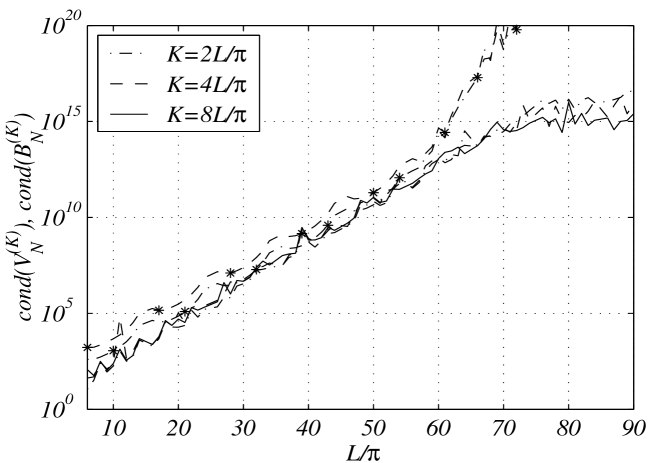
Figure 8: Dependence of condition numbers of $V_{N}^{(K)}$ and $\widetilde{{\cal B}_{N}}^{(K)}$ (marked with asterisks) on $L$ for $\gamma=0.8$.

The graph of ${\rm cond}_{2}\left(\widetilde{{\cal B}_{N}}^{(K)}\right)$ versus $L$ is also illustrated in Fig 8. Unlike $\kappa_{2}({\cal A}_{N})$, which estimates the upper bound of amplification of solutions of the initial-value problem for (5), the number ${\rm cond}_{2}\left(\widetilde{{\cal B}_{N}}^{(K)}\right)$ gives an estimation of possible amplification of perturbations of the right hand side $f$ in the solution $u_{f}$ of the linear equation $\widetilde{{\cal B}_{N}}^{(K)}u=f$. Note, because of $x$- and $\Phi$-shift invariance of (1), condition number of $\widetilde{{\cal A}_{N}}^{(K)}$ itself is infinite.

5 Comparison of the estimations

It was established in numerical experiments, see e.g. [3], [4], that for small enough computational domains of size $L<L_{c}$ numerical solutions of (1) stabilize to the steady coalescent $N_{L}$-pole solutions of (1). This observation is in the explicit agreement with the eigenvalue analysis of the linearized problem carried out in [5].

For larger $L>L_{c}$, numerical solutions do not stabilize to any steady solution at all. Instead, being essentially nonsteady, they remain very closely to the steady coalescent $N_{L}$-pole solution, developing on the surface of the flame front small cusps randomly in time. With time these small cusps move towards the trough of the flame front profile and disappear in it as can be seen in Fig. 2.

Numerous numerical experiments did not reveal any significant dependence of the critical length $L_{c}$ on parameters of the computational algorithm. They have shown, however, that $L_{c}$ is effectively affected by the round-off errors [6]. Thus, if $f$ is the order of the amplitude of perturbations associated with the round-off errors, then $L_{c}=L_{c}(f)$. Two values of $L_{c}(f)$ obtained in our calculations with 32- and 64-bit arithmetic are shown in Fig. 9. Amplitude $f$ of the perturbations was of the order of machine zeros, i.e. $10^{-7}$ and $10^{-16}$ correspondingly. Note, that in calculations with 32-bit arithmetic round-off errors dominated discretization errors [20].

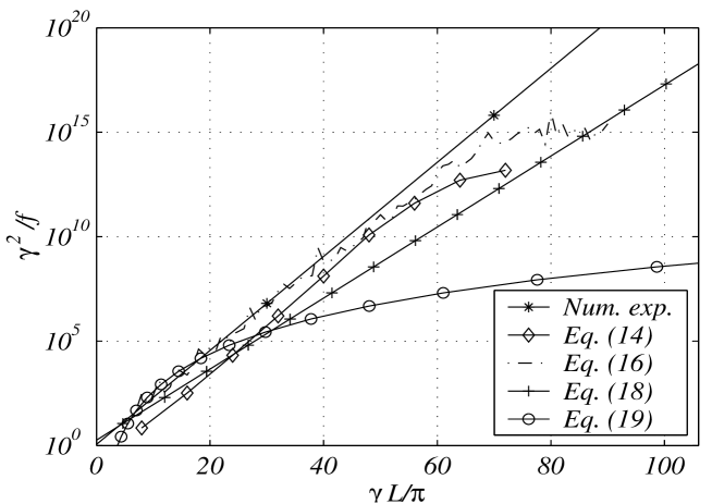
Figure 9: Dependence of the variety of measures of the critical strength $f_{c}$ of perturbations on the flame size $L$.

It is convenient to invert the relation $L_{c}=L_{c}(f)$ and write it in the form $f_{c}=f_{c}(L)$, where $f_{c}$ is a critical noise strength for given size $L$ of the flame. Reciprocal of the Kreiss constant ${\cal K}_{{\cal A}_{N}}$, obtained in Section 4.1, can be considered as the lower bound of this critical strength $f_{c}$ of perturbations for any particular value of $L$. Here, the strength of the perturbation means its 2-norm. Corresponding graph is plotted in Fig. 9. It is in a very good agreement with the results of our direct numerical simulations. The graph of $\kappa_{2}\left(\widetilde{{\cal A}_{N}}^{(K)}\right)$ versus $L$ is also given in Fig. 9, for the illustrative purposes. We remind, that there was no evidence of convergence of $\kappa_{2}\left(\widetilde{{\cal A}_{N}}^{(K)}\right)$ to $\kappa_{2}\left({\cal A}_{N}\right)$ in our calculations and interpretation of the graph as the upper bound (16) of $f_{c}$ is not justified.

An analytical attempt to estimate the value of $f_{c}$ was made in [7] where the following modification of (5), (6) has been considered:

$$\frac{\partial\phi}{\partial t}=\frac{x}{R_{N}}\frac{\partial\phi}{\partial x}+\frac{\partial^{2}\phi}{\partial x^{2}}+\frac{\gamma}{2}\frac{\partial{\cal H}[\phi]}{\partial x},\qquad x\in\mbox{\boldmath${R}$}.$$ (17)

Here $R_{N}=\left(\partial^{2}\Phi_{N}/\partial x^{2}\right)^{-1}$ is calculated in the crest of the steady coalescent $N$-pole solution, see Fig. 2. In [7] a particular asymptotic solution to (17) has been investigated. As a result, the dependence between the critical value of curvature radius $R_{N}$ in the crest of the flame profile and the spectral density $\rho_{f}$ of the most dangerous harmonics of $\phi(x,0)$ has been obtained. A functional link between $L$ and $R_{N_{L}}$ of the steady coalescent $N_{L}$-pole solution to the Sivashinsky equation can be easily established yielding

$$\rho_{f,c}=4^{-1}\gamma^{2}e^{-\gamma^{2}(c_{1}L+c_{2})/8}.$$ (18)

Here $c_{1}$ and $c_{2}$ are coefficients of the least squares fitting of $R_{N_{L}}=R_{N_{L}}(L)$ with a straight line $c_{1}L+c_{2}$.

When comparing our results with estimation (18), the following should be taken into account. First, relation (18) has been obtained for the spectral density of the most dangerous harmonics of the perturbation $\phi(x,0)$ rather than for its amplitude $f$. Second, assumptions made to obtain (18) are better justified for large $L$. The last but not least factor is that (18) is based on a particular solution and is likely to produce an overestimated value of $\rho_{f,c}$ rather than the optimal one. In view of these peculiarities, the agreement between (18), obtained in [7], and our estimations is striking.

In contrast, the estimation of $f_{c}$ obtained in [9] is obviously out of the harmony. That estimation was based on studies of the dynamics of poles governed by (3), (4). Namely, the amplitude of perturbations to the solutions of (1) was linked to the $b$-coordinate of poles in the $(a,b)$-plane. Then, analysis of the dynamics of these noise generated poles yields the estimation

$$f_{c}=2^{11}\pi^{6}\gamma^{-5}L^{-6}.$$ (19)

There is no doubt that the sensitivity of system (3), (4) to noise is totally different of what we have for (1). Analysis of the Jacobian of the right hand sides of system (3), (4) for the steady coalescent $N_{L}$-pole solution reveals that this is a symmetric matrix and there is no linear nonmodal amplification of noise in (3), (4) at all. For small $L$, when the nonmodal amplification is not essential, estimation (19) is in a good agreement with other data indeed. However, for larger $L$, the discrepancy between the results of [9] and of others, clearly seen in Fig. 9, can be interpreted as the measure of the importance of the linear nonmodal amplification of perturbations in the Sivashinsky equation.

6 Conclusions

In this paper we have undertaken the numerical analysis of norms of the resolvent of the linear operator associated with the Sivashinsky equation linearized in a neighbourhood of the steady coalescent pole solutions. Performance of available numerical techniques was compared to each other and the results are checked versus directly calculated norms of the evolution operator.

The studies demonstrated the robustness of the approach by resolving the problem of stability of certain types of cellular flames. They showed that the round-off errors are the only effect relevant to the appearance of the micro cusps in computations of large enough flames. These essentially nonlinear micro cusps are generated through the huge linear nonmodal transitional amplification of the round-off errors. Their final appearance and dynamics on the flame surface is governed by essentially nonlinear mechanisms intrinsic to the Sivashinsky equation.

In order to retain its physical meaning for large flames, Sivashinsky equation should be refined by accounting for the physical noise, e.g. in the way suggested in [8].

7 Acknowledgements

This research was supported by the EPSRC research grant GR/R66692.

References

- [1] G.I. Sivashinsky. Nonlinear analysis of hydrodynamic instability in laminar flames - I. Derivation of basic equations. Acta Astronautica, 4:1177–1206, 1977.
- [2] O. Thual, U. Frisch, and M. Hénon. Application of pole decomposition to an equation governing the dynamics of wrinkled flame fronts. Le Journal de Physique, 46(9):1485–1494, Septembre 1985.
- [3] M. Rahibe, N. Aubry, and G.I. Sivashinsky. Stability of pole solutions for planar propagating flames. Physical Review E, 54(5):4958–4972, Novenber 1996.
- [4] M. Rahibe, N. Aubry, and G.I. Sivashinsky. Instability of pole solutions for planar propagating flames in sufficiently large domains. Combustion Theory and Modelling, 2(1):19–41, March 1998.
- [5] D. Vaynblat and M. Matalon. Stability of pole solutions for planar propagating flames: I. Exact eigenvalues and eigenfunctions. SIAM Journal on Applied Mathematics, 60(2):679–702, 2000.
- [6] V. Karlin. Cellular flames may exhibit a nonmodal transient instability. Proceedings of the Combustion Institute, 29(2):1537–1542, 2002.
- [7] G. Joulin. On the hydrodynamic stability of curved premixed flames. J. Phys. France, 50:1069–1082, Mai 1989.
- [8] P. Cambray and G. Joulin. On moderately-forced premixed flames. In Twenty–Fourth Symposium (International) on Combustion, pages 61–67. The Combustion Institute, 1992.
- [9] Z. Olami, B. Galanti, O. Kupervasser, and I. Procaccia. Random noise and pole dynamics in unstable front dynamics. Physical Review E, 55(3):2649–2663, March 1997.
- [10] L.N. Trefethen, A.E. Trefethen, S.C. Reddy, and T.A. Driscoll. Hydrodynamic stability without eigenvalues. Science, 261:578–584, 30 July 1993.
- [11] L. Boberg and U. Brosa. Onset of turbulence in a pipe. Zeitschrift für Naturforschung, 43a:697–726, 1988.
- [12] S.C. Reddy, P.J. Schmid, and D.S. Henningson. Pseudospectra of the Orr-Sommerfeld operator. SIAM Journal on Applied Mathematics, 53(1):15–47, February 1993.
- [13] L.N. Trefethen. Pseudospectra of linear operators. SIAM Review, 39(3):383–406, September 1997.
- [14] L.N. Trefethen. Computation of pseudospectra. In Acta Numerica, volume 8, pages 247–295. Cambridge University Press, 1999.
- [15] A.P. Prudnikov, Yu.A. Brichkov, and O.I. Marichev. Integrals and Series, volume 1. Nauka, Moscow, 1981.
- [16] S.H. Lui. Computation of pseudospectra by continuation. SIAM Journal on Scientific Computing, 18(2):565–573, March 1997.
- [17] T.G. Wright and L.N. Trefethen. Large-scale computation of pseudospectra using ARPACK and Eigs. SIAM Journal on Scientific Computing, 23(2):591–605, 2001.
- [18] J.H. Wilkinson. The Algebraic Eigenvalue Problem. Clarendon Press, Oxford, 1965.
- [19] A. Pazy. Semigroups of Linear Operators and Applications to Partial Differential Equations. Springer Verlag, 1983.
- [20] V. Karlin, V. Maz’ya, and G. Schmidt. High accuracy periodic solutions to the Sivashinsky equation. Journal of Computational Physics, 188(1):209–231, 2003.