Using Atomic Diffraction of Na from Material Gratings to Measure Atom-Surface Interactions

Abstract

In atom optics a material structure is commonly regarded as an amplitude mask for atom waves. However, atomic diffraction patterns formed using material gratings indicate that material structures also operate as phase masks. In this study a well collimated beam of sodium atoms is used to illuminate a silicon nitride grating with a period of 100 nm. During passage through the grating slots atoms acquire a phase shift due to the van der Waals interaction with the grating walls. As a result the relative intensities of the matter-wave diffraction peaks deviate from those expected for a purely absorbing grating. Thus a complex transmission function is required to explain the observed diffraction envelopes. An optics perspective to the theory of atomic diffraction from material gratings is put forth in the hopes of providing a more intuitive picture concerning the influence of the vdW potential. The van der Waals coefficient $C_{3}=2.7\pm 0.8\mbox{\ meV\ nm}^{3}$ is determined by fitting a modified Fresnel optical theory to the experimental data. This value of $C_{3}$ is consistent with a van der Waals interaction between atomic sodium and a silicon nitride surface.

It is known that correlations of electromagnetic vacuum field fluctuations over short distances can result in an attractive potential between atoms. For the case of an atom and a surface the potential takes the form

$$\begin{split}V(r)&=-\frac{C_{3}}{r^{3}},\end{split}$$ (1)

where $r$ is the atom-surface distance and $C_{3}$ is a coefficient which describes the strength of the van der Waals (vdW) interaction Milonni (1994). Equation 1 is often called the non-retarded vdW potential and is valid over distances shorter than the principle transition wavelength of the atoms involved. The significance of this interaction is becoming more prevalent as mechanical structures are being built on the nanometer scale. The vdW potential also plays an important part in chemistry, atomic force microscopy, and can be used to test quantum electrodynamic theory.

Early experiments concerning the vdW interaction were based on the deflection of atomic beams from surfaces. It was demonstrated that the deflection of ground state alkali Shih and Parsegian (1975) and Rydberg Anderson et al. (1988) atom beams from a gold surface is compatible with Eq. 1. Later measurements based on the Stark shift interpretation of the vdW potential Sukenik et al. (1993) were sufficiently accurate to distinguish between the retarded $V\sim r^{-4}$ and non-retarded $V\sim r^{-3}$ forms. More recently atom optics techniques have been employed to measure the magnitude of the vdW coefficient $C_{3}$. Various ground state Grisenti et al. (1999) and excited noble gas Bruhl et al. (2002) atom beams have been diffracted using nano-fabricated transmission gratings in order to measure $C_{3}$. The influence of the vdW potential has also been observed for large molecules in a Talbot-Lau interferometer constructed with three gold gratings Brezger et al. (2002).

In this article we present atomic diffraction of a thermal sodium atom beam and show that the data cannot be described by a purely absorbing grating. A diagram of the experimental apparatus is shown in Fig. 1.

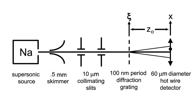
Figure 1: A diagram of the experimental setup used.

The supersonic beam of sodium atoms passes through a .5 mm diameter skimmer and is collimated by two $\mbox{10\ }\mu\mbox{m}$ slits separated by $\sim 1\mbox{\ m}$. By changing the carrier gas the atom velocity can be adjusted from 0.6 to 3 km/s with $\frac{\sigma_{v}}{v}\sim.1$. The collimated atom beam is used to illuminate a silicon nitride grating Savas et al. (1996) with a period of $d=100\mbox{\ nm}$, thickness $t=150\pm 5\mbox{\ nm}$, open width $w=50.5\pm 1.5\mbox{\ nm}$, and grating bar wedge angle $\alpha=5.25\pm.75$ degrees. All of the grating parameters are measured independently using scanning electron microscope images. The diffraction pattern is measured by ionizing the sodium atoms with a hot Re wire and then counting the ions with a channel electron multiplier.

An optical description is helpful in gaining an intuitive picture of how the vdW interaction modifies the atomic diffraction pattern. To this end one should recall that the Schroedinger equation for a wave function $\psi$ can be written as

$$\begin{split}i\hbar\frac{\partial}{\partial t}\psi(\mbox{\bf{r}},t)&=\left[\frac{-\hbar^{2}}{2m}\nabla^{2}+V(\mbox{\bf{r}})\right]\psi(\mbox{\bf{r}},t),\end{split}$$ (2)

where $m$ is mass, $\hbar$ is Planck’s constant, and $V$ is the potential Griffiths (1995). One can take the Fourier transform of Eq. 2 with respect to time and use the fact that $\frac{\partial}{\partial t}\Rightarrow-i\omega$ in the frequency domain to obtain

$$\begin{split}\left[\nabla^{2}+\left(1-\frac{V(\mbox{\bf{r}})}{\hbar\omega}\right)k_{o}^{2}\right]\psi(\mbox{\bf{r}},\omega)&=0,\end{split}$$ (3)

where the dispersion relation $\omega=\frac{\hbar k_{o}^{2}}{2m}$ has been utilized. Equation 3 is usually referred to as the time independent Schroedinger equation. It is quite illuminating to recall that the Helmholtz equation Jackson (1999) for the electric field E is given by

$$\begin{split}\left(\nabla^{2}+n^{2}k_{o}^{2}\right)\mbox{\bf{E}}(\mbox{\bf{r}},\omega)=0,\end{split}$$ (4)

where $n$ is index of refraction. By inspection one can see that Eqs. 3 and 4 are formally equivalent where the quantities $n$ and $\left(1-\frac{V}{\hbar\omega}\right)^{1/2}$ play analogous roles. Due to this fact many wave propagation methods developed in optics can be applied directly to matter wave propagation, being mindful of the fact that in optics $\omega=ck_{o}$.

While Eq. 3 can be formally solved using a Green’s function approach, approximate solutions used in physical optics can lead to a better understanding of how the vdW interaction affects atomic diffraction patterns. The Fresnel and Fraunhofer approximations are commonly used in optics and represent a useful tool when faced with propagating the wave function $\psi$ from the grating to the detector plane. The Fresnel or paraxial approximation is valid as long as the propagation distance $z$ satisfies the inequality

$$\begin{split}z\gg|x-\xi|.\end{split}$$ (5)

This is certainly satisfied for our experiment since the diffraction angles are less than $10^{-3}$ radians and the orders are resolved. The Fraunhofer or far-field approximation goes beyond the Fresnel approximation by requiring that

$$\begin{split}z\gg\frac{k_{o}}{2}\xi_{max}^{2}=\frac{\pi}{\lambda_{dB}}\xi_{max}^{2},\end{split}$$ (6)

where $\lambda_{dB}$ is the de Brolglie wavelength of the atoms and $\xi_{max}$ is the relevant extent in the aperture plane Goodman (1996). For the case of propagation from a uniformly illuminated grating of period $d$ to the detector plane, $\xi_{max}\rightarrow d$ and Eq. 6 takes the form $z\gg\frac{\pi d^{2}}{\lambda_{dB}}$. For our experimental setup $d=100\mbox{\ nm}$ and $\lambda_{dB}\sim 10^{-11}\mbox{\ m}$, so the inequality $z\approx 2\mbox{\ m}\gg\frac{\pi}{1000}\mbox{\ m}$ is met. However, our atom beam diameter is on the order of $10^{-5}$ m and so $\xi_{max}\rightarrow 10^{-5}$ m implying that the inequality in Eq. 6 is not met.

In light of the previous discussion it seems most appropriate to use the Fresnel approximation to model our experiment. According to the Fresnel approximation the wave function in the detector plane $\psi(x)$ is related to that just after the grating $\psi(\xi)$ by a scaled spatial Fourier transform

$$\begin{split}\psi(x)&\propto\left.\mathcal{F}\left\{e^{i\frac{k_{o}\xi^{2}}{2z_{o}}}\psi(\xi)\right\}\right|_{f_{\xi}=\frac{x}{\lambda_{dB}z_{o}}},\end{split}$$ (7)

where $\mathcal{F}\{\}$ denotes a Fourier transform and $f_{\xi}$ is the Fourier conjugate variable to $\xi$ Goodman (1996). The quadratic phase factor in Eq. 7 accounts for the fact that the phase fronts have a parabolic shape before the far-field is reached.

The wave function just after the grating $\psi(\xi)$ is given by

$$\begin{split}\psi(\xi)&=\left[T(\xi)\ast\mbox{comb}\left(\frac{\xi}{d}\right)\right]U(\xi),\end{split}$$ (8)

where $\mbox{comb}\left(\frac{\xi}{d}\right)$ is an array of delta functions with spacing $d$, the operator $\ast$ denotes a convolution, and $U(\xi)$ is complex function describing the atom beam amplitude in the plane of the grating. The transmission function of a single grating window $T(\xi)$ in Eq. 8 is defined as

$$\begin{split}T(\xi)&\equiv e^{i\phi(\xi)}\mbox{rect}\left(\frac{\xi}{w}\right),\end{split}$$ (9)

where $\mbox{rect}(arg)=1$ when $|arg|\leq\frac{1}{2}$ and zero otherwise. The phase $\phi(\xi)$ accounts for the vdW interaction and its origin will be discussed later. This description of $\psi(\xi)$ and $T(\xi)$ in terms of the functions comb() and rect() is standard Fourier optics notation and convenient due to its modular nature Goodman (1996).

Equation 8 can then be substituted into Eq. 7 to obtain

$$\begin{split}\psi(x)&\propto\sum_{j=-\infty}^{\infty}\mathcal{A}_{j}U\left(x-j\frac{\lambda_{dB}z_{o}}{d}\right),\end{split}$$ (10)

where the summation index corresponds to the $j^{th}$ diffraction order, the diffraction amplitude $\mathcal{A}_{j}$ is defined as

$$\begin{split}\mathcal{A}_{j}&\equiv\left.\mathcal{F}\left\{T(\xi)\right\}\right|_{f_{\xi}=\frac{j}{d}}=\left.\mathcal{F}\left\{e^{i\phi(\xi)}\mbox{rect}\left(\frac{\xi}{w}\right)\right\}\right|_{f_{\xi}=\frac{j}{d}},\end{split}$$ (11)

and the beam profile in the detector plane is given by

$$\begin{split}U(x)=\left.\mathcal{F}\left\{e^{i\frac{k_{o}\xi^{2}}{2z_{o}}}U(\xi)\right\}\right|_{f_{\xi}=\frac{x}{\lambda_{dB}z_{o}}}.\end{split}$$ (12)

From Eq. 10 we can predict the atom intensity

$$\begin{split}I(x)\equiv\left|\psi(x)\right|^{2},\end{split}$$ (13)

in the detector plane which can also be interpreted as the probability law for atoms. A distribution of atom velocities can be incorporated by a weighted incoherent sum of the intensity pattern for each atom velocity $I\left(x;v\right)$

$$\begin{split}I(x)&=\sum_{v}P(v)I\left(x;v\right);\qquad v=\frac{h}{m\lambda_{dB}},\end{split}$$ (14)

$$\begin{split}P(v)&\propto v^{3}exp\left(-\frac{m(v-u)^{2}}{2k_{B}T}\right),\end{split}$$ (15)

where the $P(v)$ is the probability distribution function of velocities for a supersonic source, $u$ is the average flow velocity, $k_{B}$ is Boltzmann’s constant, and $T$ is the longitudinal temperature of the beam in the moving frame of the atoms Dunning and Hulet (1996).

One can see from Eq. 10 that the diffraction pattern consists of replications of the beam shape $\left|U(x)\right|^{2}$ shifted by integer multiples of $\frac{\lambda_{dB}z_{o}}{d}$ with relative intensities determined by the modulus squared of Eq. 11. An important feature to notice in Eq. 11 is that a diffraction order in the detector plane corresponds to a spatial frequency in the grating plane through the relation $f_{\xi}=\frac{j}{d}$. This highlights the connection between the spatially dependent phase $\phi(\xi)$ in Eq. 9 and the magnitude of the diffraction orders in Eq. 10.

The earlier assertion that $\phi(\xi)$ in Eq. 9 somehow incorporates the vdW interaction into the optical propagation theory can be understood by recalling from Eq. 3 that the index of refraction $n$ and quantity $\left(1-\frac{V}{\hbar\omega}\right)^{1/2}$ play similar roles in optics and atom optics, respectively. In optics one calculates a phase shift $\phi$ induced by a glass plate by multiplying the wavenumber in the material $nk_{o}$ by the thickness of the plate $L$ (i.e. $\phi=nk_{o}L$). Just as in the optics case one can calculate the phase shift $\phi(\xi)$ accumulated by the wave function passing through the grating windows

$$\begin{split}\phi(\xi)&=\int\left(\parbox{54.2025pt}{wavenumber in potential}\right)\left(\parbox{46.97505pt}{differential thickness}\right)\\ &=\int_{-t}^{0}k_{o}\left(1-\frac{V(\xi,z)}{\hbar\omega}\right)^{1/2}dz,\end{split}$$ (16)

where $t$ is the thickness of the grating and $V(\xi,z)$ is the potential the atoms experience between the grating bars due to the vdW interaction. Thus the vdW interaction is analogous to a glass plate with a spatially dependent index of refraction, a kind of diverging lens that fills each grating window. The result in Eq. 16 is consistent with the wave function phase according to the WKB approximation Griffiths (1995).

In arriving at Eq. 16 diffraction due to abrupt changes in the potential $V(\xi,z)$ has been ignored while the wave function propagates through the grating windows. This is a valid approximation due to the fact that $\lambda_{dB}\ll w,\left[\frac{\partial}{\partial\xi}\frac{V(\xi)}{\hbar\omega}\right]^{-1}$ in the region of the potential that corresponds to the diffraction orders of interest. The relationship between spatial regions of the potential $V(\xi,z)$ and a given diffraction order will be discussed in subsequent paragraphs. It is also important to note that Eq. 16 assumes that the potential $V(\xi,z)$ exists only between the grating bars (i.e. $V(\xi,z)=0$ for $z<-t$ or $z>0$) and neglects the fact that the bars are not semi-infinite planes. Theoretical work done by Spurch et al. Zhou and Spruch (1995) suggests that the vdW potential corresponding to our $\sim 50$ nm grating bar width is very similar to that of a semi-infinite plane in the $\xi$ direction. Since the phase $\phi(\xi)$ from Eq. 16 only depends on the integral of the potential in the $z$ direction one would also expect that edge effects in $V(\xi,z)$ due to the finite grating thickness $t$ are a small correction.

If the particle energy $\hbar\omega$ is much greater than the potential $V(\xi,z)$ then Eq. 16 can be further simplified by Taylor expanding the quantity $\left(1-\frac{V}{\hbar\omega}\right)^{1/2}$ and keeping the leading order term in $\frac{V}{\hbar\omega}$

$$\begin{split}\phi(\xi)=tk_{o}-\frac{1}{\hbar v}\int_{-t}^{0}V(\xi,z)dz;\qquad\hbar\omega\gg V(\xi,z),\end{split}$$ (17)

through the use of the dispersion relation $\omega=\frac{\hbar k_{o}^{2}}{2m}$ and $p=mv=\hbar k_{o}$. Equation 17 is often called the Eikonal approximation. The term $tk_{o}$ in Eq. 17 is independent of $\xi$ and of no consequence in Eq. 11 so it can be neglected. One can see from Eq. 17 that if $V(\xi,z)\rightarrow 0$ then Eq. 11 reduces to the sinc diffraction envelope expected from a purely absorbing grating. Furthermore, it is now clear from Eqs. 11 and 17 that the relative heights of the diffraction orders are altered in a way that depends on $V(\xi,z)$ as well as the atom beam velocity $v$.

As a simple model one can represent the potenial in Eq. 17 as the sum of the potential due to the two interior walls of the grating window

$$\begin{split}\phi(\xi)=-\frac{t}{\hbar v}\left[g_{-}(\alpha)V_{-}(\xi)-g_{+}(\alpha)V_{+}(\xi)\right],\end{split}$$ (18)

where the function $g_{\pm}(\alpha)$ incorporates the influence of the wedge angle $\alpha$

$$\begin{split}g_{\pm}(\alpha)\equiv\frac{1\pm\frac{t\tan\alpha}{2\left(\xi\pm\frac{w}{2}\right)}}{\left(1\pm\frac{t\tan\alpha}{\left(\xi\pm\frac{w}{2}\right)}\right)^{2}},\end{split}$$ (19)

and $V_{\pm}(\xi)\equiv C_{3}\left(\xi\pm\frac{w}{2}\right)^{-3}$ is implied by Eq. 1. Equations 18 and 19 are arrived at by carrying out the integration in Eq. 17 while assuming that the open grating width $w$ varies in the propagation direction $z$ as $w(z)=w+2z\tan\alpha$. Since the principle transition wavelength of Na (590 nm) is much larger than $\frac{w}{2}$ (i.e. the maximum atom-surface distance of $\sim 25$ nm) the non-retarded form of the vdW potential is appropriate.

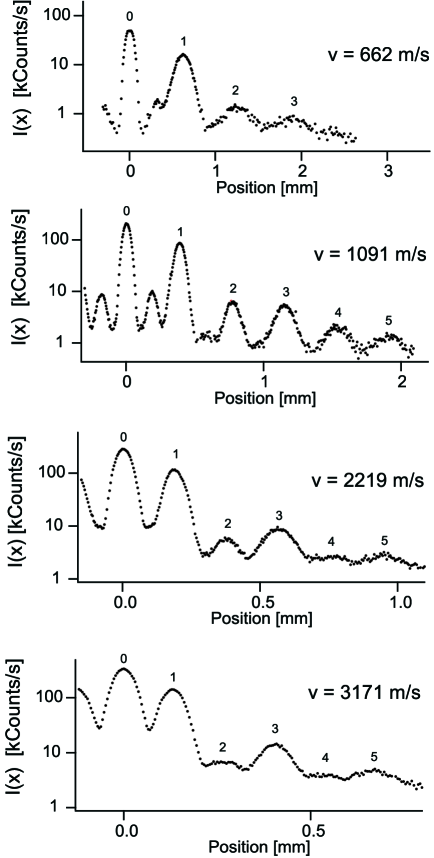
Figure 2: Observed diffraction patterns of four different atom velocities. The numbers next to the peaks indicate the diffraction order. Molecular $\mbox{Na}_{2}$ peaks are also visible between zeroth and first orders for slower velocities.

It is not immediately obvious how the phase representation in Eq. 17 will affect the far-field diffraction pattern or if the Eikonal approximation is appropriate in light of Eq. 18 (i.e. $V_{\pm}(\xi)\rightarrow-\infty$ as $|\xi|\rightarrow\frac{w}{2}$). In order to address this it is helpful to introduce the concept of an instantaneous spatial frequency Boyd (1992)

$$\begin{split}f_{\xi}\left(\xi_{j}\right)\equiv\left.\frac{\partial\phi}{\partial\xi}\right|_{\xi=\xi_{j}}=\frac{j}{d},\end{split}$$ (20)

where $\xi_{j}$ is the grating window location corresponding to the diffraction order $j$ as in Eq. 11. For the limiting case of $\alpha\rightarrow 0$ the geometry factor $g_{\pm}(\alpha)\rightarrow 1$ the higher order terms in Eq. 16 will become important when $\xi_{j}\rightarrow\xi_{c}$ and $C_{3}\left(\xi_{c}-\frac{w}{2}\right)^{-3}\approx\hbar\omega$. If Eq. 18 is inserted into Eq. 20 with the previously mentioned limits one can solve for the diffraction order $j_{c}$ at which the approximation in Eq. 17 breaks down

$$\begin{split}j_{c}&\approx\frac{3k_{o}t}{2}\frac{C_{3}d}{\hbar\omega\left(\xi_{c}-\frac{w}{2}\right)^{4}}=\frac{3k_{o}t}{2}\left(\frac{d^{3}\hbar\omega}{C_{3}}\right)^{\frac{1}{3}}.\end{split}$$ (21)

For the present experiment $\frac{3k_{o}t}{2}\sim 10^{5}$ and $\left(\frac{d^{3}\hbar\omega}{C_{3}}\right)^{\frac{1}{3}}\sim 10^{\frac{7}{3}}$ which implies that $j_{c}\sim 10^{7}$. Thus the approximation in Eq. 17 is appropriate since we typically concerned with only the first ten diffraction orders. In fact, the paraxial approximation will become invalid before Eq. 17 becomes invalid due to the fact the diffraction order spacing is typically $\frac{\lambda_{dB}z_{o}}{d}\sim.1\mbox{\ mm}$. It is also interesting to note that using Eqs. 18 and 20 one can solve for the position $\xi_{j}$ in the grating window

$$\begin{split}\xi_{j}\approx\frac{w}{2}-\left(\frac{3tC_{3}d}{j\hbar v}\right)^{\frac{1}{4}};\quad j\geq 1,\end{split}$$ (22)

corresponding to a particular diffraction order $j$. If $j=1$ in Eq. 22 then $\xi_{1}\approx 3.2$ nm and since $\xi_{j}\sim j^{-\frac{1}{4}}$ the shape of the diffraction amplitude in Eq. 11 depends on a small region of the potential near an an atom-surface distance of $\sim 20$ nm.

The experimental data for diffraction patterns of four different atom beam velocities are displayed in Fig. 2. One can see from Fig. 2 that the second order diffraction peak is almost completely suppressed for the faster atoms whereas it is quite pronounced for the slower atoms. This velocity dependence is a clear indication that a complex transmission functions such as Eq. 9 (i.e. $C_{3}\neq 0$) is required to explain the data. A least-squares fit to Eqs. 10 and 14 is used to determine diffraction envelope $\left|\mathcal{A}_{j}\right|^{2}$ and the average velocity. It is clear from Fig. 2 that the diffraction orders overlap to some extent, hence the tails of the beam shape are important when determining $\left|\mathcal{A}_{j}\right|^{2}$. The broad tails of the beam shape were not adequately described by a Gaussian so an empirical shape using a fixed collimating geometry was derived from the measured raw beam profile and used for $\left|U(x)\right|^{2}$.

The diffraction amplitudes $\left|\mathcal{A}_{j}\right|^{2}$ determined from Fig. 2 for the various velocities are displayed in Fig. 3. The vdW coefficient $C_{3}$ is determined by a least-squares fit to this reduced data with the modulus squared of Eq. 11. All of the grating parameters are determined independently, therefore $C_{3}$ is the only free parameter. Data from each velocity is fit simultaneously with the same $C_{3}$. It is clear that a purely absorbing grating (i.e. $C_{3}=0$) is inconsistent with all of the observed $\left|\mathcal{A}_{j}\right|^{2}$ especially at lower velocities for which the phase $\phi(\xi)$ is much larger. Uncertainty in the determination of the grating parameter $w$ and the exact shape of the potential in Eq. 17 may be responsible for the slight deviation from theory evident in Fig. 3.

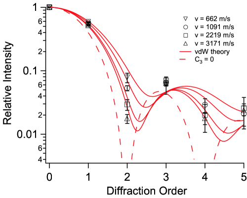
Figure 3: Diffraction order intensities and best fit diffraction amplitude $\left|\mathcal{A}_{j}\right|^{2}$. Notice how the theory for a purely absorbing grating fails to describe the data.

A study of the systematic errors in our experiment and analysis suggest that $w$ is largest source of uncertainty when calculating $C_{3}$. One can numerically calculate the function ${C}_{3}(w)$, which is the best fit $C_{3}$ as a function of $w$, whose linear dependence around the physical value of $w$ is found to be $\left.\frac{\partial C_{3}}{\partial w}\right|_{w=50.5\mbox{\ }nm}=.52\mbox{\ }\mbox{\ meV\ nm}^{2}$. The error in $C_{3}$ is arrived at by taking the product of this slope and the 1.5 nm uncertainty in $w$. After carrying out the previously described analysis we obtain a value for the vdW coefficient $C_{3}=2.7\pm 0.8\mbox{\ }\mbox{\ meV\ nm}^{3}$. The uncertainty determined this way is considerably larger than the statistical uncertainty in $C_{3}$ from the least-squares fitting procedure. The uncertainty due to $w$ is also larger than the systematic corrections due to the atom beam profile or uncertainties due to imperfect knowledge of the grating parameters: $d$, $t$, and $\alpha$.

Table 1: Measured and calculated values of $C_{3}$

Method	$C_{3}\ \left[\mbox{\ meV\ nm}^{3}\right]$
This experiment	$2.7\pm 0.8$
Na and perfect conductor Derevianko et al. (1999)	7.60
Na† and perfect conductor Marinescu et al. (1997); Lifshitz (1956); Meystre and Sargent (1998)	6.29
Na† and Na surface	4.1
Na† and SiNx surface	3.2
Na† and SiNx with a 1-nm Na layer§	3.8

^† indicates a one-oscillator model for atomic polarizability.
^§ indicates $C_{3}$ evaluated $20$ nm from the first surface.

To compare our experimental measurement with theoretical predictions of the van der Waal potential strength, we evaluate five different theoretical cases for sodium atoms and various surfaces in Table 1. The Lifshitz formula Lifshitz (1956) for $C_{3}$ is

$$C_{3}=\frac{\hbar}{4\pi}\int_{0}^{\infty}d\omega\alpha(i\omega)\frac{\epsilon(i\omega)-1}{\epsilon(i\omega)+1},$$ (23)

where $\alpha(i\omega)$ is the dynamic polarizability of the atom and $\epsilon(iw)$ is the permittivity of the surface material, both of which are a function of complex frequency.

A single Lorentz oscillator model for an atom (i.e. neglecting all but the valence electron) with no damping gives an expression for polarizability Meystre and Sargent (1998)

$$\alpha(i\omega)=\frac{\alpha(0)}{1+(\frac{\omega}{\omega_{0}})^{2}}.$$ (24)

For sodium atoms $\alpha(0)=24.1\ \AA^{3}$ Ekstrom et al. (1995) and $\omega_{0}=2\pi c/(590\ \mbox{nm})$. Combining this with a perfect conductor (i.e. $\epsilon=\infty$) in Eq. 23 gives $C_{3}=6.29\ \mbox{meV nm}^{3}$. This value agrees well with the non-retarded limit calculated in reference Marinescu et al. (1997) for sodium atoms with a single valence electron.

For more accurately modeled sodium atoms and a perfect conductor, Derevianko $et$ $al.$ Derevianko et al. (1999) calculated $C_{3}=7.60\ \mbox{meV nm}^{3}$ and reported a range of values spanning $0.08\ \mbox{meV nm}^{3}$ based on different many-body calculation methods which all include the effect of core electrons. It is noteworthy that $16\%$ of this recommended value is due to the core electrons Derevianko et al. (1999).

For a metal surface, the Drude model describes $\epsilon(i\omega)$ in terms of the plasma frequency and damping:

$$\epsilon(i\omega)=1+\frac{\omega_{p}^{2}}{\omega(\omega+\gamma)}.$$ (25)

For sodium metal, $\hbar\omega_{p}=5.8\ \mbox{eV}$ and $\hbar\gamma=23\ \mbox{meV},$ resulting in $C_{3}=4.1\ \mbox{meV nm}^{3}$ for a sodium atom and a bulk sodium surface. Presumably this calculation also under-estimates $C_{3}$ because the core electrons are neglected. However, the calculation error is probably smaller than that of a perfect conductor because the core electron excitations are at frequencies comparable to $\omega_{p}$.

For an insulating surface of silicon nitride, which is the diffraction grating material, Bruhl $et$ $al$ Bruhl et al. (2002) used a model with

$$\epsilon(i\omega)=\frac{\omega^{2}+(1+g_{0})\omega_{0}^{2}}{\omega^{2}+(1-g_{0})\omega_{0}^{2}}$$ (26)

where $\hbar\omega_{0}\equiv E_{s}=13\mbox{eV}$ and $g_{0}=0.588$ is the material response function at zero frequency. Using Eqs. 23, 24, and 26 gives a value of $C_{3}=3.2\ \mbox{meV nm}^{3}$.

A multilayered surface makes a vdW potential that no longer depends exactly on $r^{-3},$ even in the non-retarded limit. We used Equation 4.10 from reference Zhou and Spruch (1995) to calculate $V(r)$ for thin films of sodium on a slab of silicon nitride. Because our experiment is sensitive to atom-surface distances in the region 20 nm, we report the nominal value of $C_{3}$ from these calculations using $C_{3}=V(\mbox{20 nm})\times(\mbox{20 nm})^{3}$. Evaluated this way, isolated thin films make a smaller $C_{3}$ as $r$ increases. Films on a substrate make $C_{3}$ vary from the value associated with the bulk film material to the value associated with the bulk substrate material as $r$ increases.

In conclusion an optics perspective to the theory of atomic diffraction from a material grating has been put forth. The results in Eqs. 11, 17 and 18 have been derived using Fourier optics techniques and appear to be consistent with the diffraction theory presented in Grisenti et al. (2000). Diffraction data for a sodium atom beam at four different velocities show clear evidence of atom-surface interactions with the silicon nitride grating. A complex transmission function such as that in Eq. 9 is required to explain the data. The measured value of $C_{3}=2.7\pm 0.8\mbox{\ }\mbox{\ meV\ nm}^{3}$ is limited in precision by uncertainty of the grating parameter $w$. Based on the results in Table 1 for a single Lorentz oscillator the new measurement of $C_{3}$ presented in this article is consistent with a vdW interaction between atomic sodium and a silicon nitride surface. Our measurement is inconsistent with a perfectly conducting surface and also a silicon nitride surface coated with more than one nm of bulk sodium. This implies that atomic diffraction from a material grating may provide the means to test the theory of vdW interactions with a multi-layered surface Zhou and Spruch (1995) by using coated gratings.

The authors would like to thank Hermann Uys for technical assistance.

References

- Milonni (1994) P. W. Milonni, The Quantum Vacuum (Academic Press, 1994).
- Shih and Parsegian (1975) A. Shih and V. A. Parsegian, Phys. Rev. A 12, 835 (1975).
- Anderson et al. (1988) A. Anderson, S. Haroche, E. A. Hinds, J. W., and D. Meschede, Phys. Rev. A 37, 3594 (1988).
- Sukenik et al. (1993) C. I. Sukenik, M. G. Boshier, D. Cho, V. Sandoghdar, and E. A. Hinds, Phys. Rev. Lett. 70, 560 (1993).
- Grisenti et al. (1999) R. E. Grisenti, W. Schollkopf, J. P. Toennies, G. C. Hegerfeldt, and T. Kohler, Phys. Rev. Lett. 83, 1755 (1999).
- Bruhl et al. (2002) R. Bruhl, P. Fouquet, R. E. Grisenti, J. P. Toennies, G. C. Hegerfeldt, T. Kohler, M. Stoll, and D. Walter, Europhys. Lett. 59, 357 (2002).
- Brezger et al. (2002) B. Brezger, L. Hackermuller, S. Uttenthaler, J. Petschinka, M. Arndt, and A. Zeilinger, Phys. Rev. Lett. 88, 100404 (2002).
- Savas et al. (1996) T. A. Savas, M. L. Schattenburg, J. M. Carter, and H. I. Smith, J. Vac. Sci. Tech. B 14, 4167 (1996).
- Griffiths (1995) D. J. Griffiths, Introduction to Quantum Mechanics (Prentice Hall, 1995).
- Jackson (1999) J. D. Jackson, Classical Electrodynamics (John Wiley & Sons, 1999).
- Goodman (1996) J. W. Goodman, Introduction to Fourier Optics (McGraw-Hill, 1996).
- Dunning and Hulet (1996) F. B. Dunning and R. G. Hulet, eds., Atomic, Molecular, and Optical Physics: Atoms and Molecules (Academic Press, 1996).
- Zhou and Spruch (1995) F. Zhou and L. Spruch, Phys. Rev. A 52, 297 (1995).
- Boyd (1992) R. W. Boyd, Nonlinear Optics (Academic Press, 1992).
- Derevianko et al. (1999) A. Derevianko, W. Johnson, M. Safranova, and J. Baab, Phys. Ref. Lett. 82, 3589 (1999).
- Marinescu et al. (1997) M. Marinescu, A. Dalgarno, and J. Baab, Phys. Rev. A 55, 1530 (1997).
- Lifshitz (1956) Lifshitz, JETP 73 (1956).
- Meystre and Sargent (1998) P. Meystre and S. Sargent, Elements of quantum optics (1998).
- Ekstrom et al. (1995) C. Ekstrom, J. Schmiedmayer, M. Chapman, T. Hammond, and D. E. Pritchard, Phys. Rev. A 51, 3883 (1995).
- Grisenti et al. (2000) R. E. Grisenti, W. Schollkopf, J. P. Toennies, J. R. Manson, T. A. Savas, and H. I. Smith, Phys. Rev. A 61, 033608 (2000).