DOCTOR OF PHILOSOPHY

2005

UA doesn’t use this…

Nuclear Magnetic Resonance with the Distant Dipolar Field

APPROVAL FORM

THE UNIVERSITY OF ARIZONA GRADUATE COLLEGE

As members of the Dissertation Committee, we certify that we have read the dissertation prepared by Curtis Andrew Corum entitled “Nuclear Magnetic Resonance with the Distant Dipolar Field” and recommend that it be accepted as fulfilling the dissertation requirement for the Degree of Doctor of Philosophy

____________________ Date: 12/2/2004

Arthur F. Gmitro

____________________ Date: 12/2/2004

Harrison H. Barrett

____________________ Date: 12/2/2004

Theodore Trouard

____________________ Date: 12/2/2004

Jean-Phillipe Galons

Final approval and acceptance of this dissertation is contingent upon the candidate’s submission of the final copies of the dissertation to the Graduate College.

I hereby certify that I have read this dissertation prepared under my direction and recommend that it be accepted as fulfilling the dissertation requirement.

____________________ Date: 12/2/2004

Arthur F. Gmitro

STATEMENT BY AUTHOR

This dissertation has been submitted in partial fulfillment of requirements for an advanced degree at The University of Arizona and is deposited in the University Library to be made available to borrowers under rules of the Library.

Brief quotations from this dissertation are allowable without special permission, provided that accurate acknowledgment of source is made. Requests for permission for extended quotation from or reproduction of this manuscript in whole or in part may be granted by the copyright holder.

SIGNED: ____Curtis Andrew Corum____

ABSTRACT

Distant dipolar field (DDF)-based nuclear magnetic resonance is an active research area with many fundamental properties still not well understood. Already several intriguing applications have developed, like HOMOGENIZED and IDEAL spectroscopy, that allow high resolution spectra to be obtained in inhomogeneous fields, such as in-vivo. The theoretical and experimental research in this thesis concentrates on the fundamental signal properties of DDF-based sequences in the presence of relaxation ($T_{1}$ and $T_{2}$) and diffusion. A general introduction to magnetic resonance phenomenon is followed by a more in depth introduction to the DDF and its effects. A novel analytical signal equation has been developed to describe the effects of $T_{2}$ relaxation and diffusing spatially modulated longitudinal spins during the signal build period of an HOMOGENIZED cross peak. Diffusion of the longitudinal spins results in a lengthening of the effective dipolar demagnetization time, delaying the re-phasing of coupled anti-phase states in the quantum picture. In the classical picture the unwinding rate of spatially twisted magnetization is no longer constant, but decays exponentially with time. The expression is experimentally verified for the HOMOGENIZED spectrum of 100mM TSP in $H_{2}O$ at 4.7T. Equations have also been developed for the case of multiple repetition steady state 1d and 2d spectroscopic sequences with incomplete magnetization recovery, leading to spatially varying longitudinal magnetization. Experimental verification has been accomplished by imaging the profile. The equations should be found generally applicable for those interested in DDF-based spectroscopy and imaging.

Part I The Basics

Chapter 1 INTRODUCTION

1.1 Motivation and Setting

Distant dipolar field (DDF) based nuclear magnetic resonance is a relatively new area of research. It utilizes what had been thought of as the negligible interaction between macroscopic groups of spins in a liquid. This is in contrast to microscopic interactions which contribute to relaxation effects.

The macroscopic or “distant” dipolar field now becomes a new tool, added to the already overflowing toolbox of physical and physiological effects utilized in magnetic resonance spectroscopy (MRS) and imaging (MRI). It offers many exciting possibilities such novel contrast imaging, motion insensitivity [1], and mesoscale (below the size of single voxel) spatial frequency selectivity.

One of the most intriguing features, at least for in-vivo spectroscopy, is insensitivity to $B_{0}$ inhomogeneity. This was demonstrated by Warren et al. in the HOMOGENIZED 2d spectroscopy sequence [2].

The work presented in this thesis was motivated by trying to apply HOMOGENIZED to an NMR compatible bioreactor system [3]. This system has practical limits for line-widths obtainable in localized spectroscopy, which HOMOGENIZED could potentially overcome. As the work progressed it became obvious that there were still fundamental issues not well understood for HOMOGENIZED and DDF in general. The work then shifted to understanding such fundamental issues as signal dependence on $T_{1}$, $T_{2}$, and diffusion, as well as the fundamental nature and spatial origin of the signal.

1.2 Prehistory of NMR

Semantics and the lens of hindsight make any historical and even scientific historical fact open to interpretation. The field of nuclear magnetic resonance (NMR) is generally said to originate with the announcement by I. I. Rabi et al.[4, 5] of a new “resonant” technique for measuring the magnetic moment of nuclei in a molecular beam passing through a magnetic field. This became quickly established as a powerful technique for the measurement of magnetic properties of nuclei. Subsequently E. Purcell et al.[6] looked at resonant absorption of radio-frequency energy in protons in semi-solid paraffin. Nearly simultaneously F. Bloch et al.[7] reported resonant ”induction” in liquid water. These successes were preceded by earlier efforts in the Netherlands and in Russia[8]. The importance of NMR was highlighted by the awarding of the Nobel Prize for Physics to Rabi in 1944, and to Bloch and Purcell in 1952.

The infant technique of NMR in liquids and solids quickly established itself as a useful probe of numerous physical properties of nuclei, atoms and molecules in solution and solids. Over the years it has developed from a technique of experimental physics to one of experimental chemistry, to a routine analytical tool in chemistry and to some degree solid state physics and materials science. It then branched into radiology/medical imaging as Magnetic Resonance Imaging (MRI, originally called nuclear magnetic resonance imaging, the unpopular term “nuclear” being dropped).

Chapter 2 NUCLEAR MAGNETISM

2.1 The NMR Phenomenon

The matter that surrounds us is composed of atoms and molecules, arranged as atomic or molecular gas mixtures (the atmosphere), liquid mixtures or solutions (the ocean, lakes, tap water, gasoline, urine), liquid crystals, solids (rocks, metals, glasses, etc.), plasmas (consisting of partly or wholly ionized atoms and molecules) and more complicated suspensions, composites, and living systems. All atoms in all these states of matter contain a nucleus and some of these nuclei (those with an odd number of protons or neutrons) possess a net spin and a magnetic moment [9, section 1.3.3, pp 12-15]. The magnitude of the proton and other nuclear magnetic moments has been measured to great accuracy thanks to the resonant atomic beam experiments of Rabi et al. [5] and followers. The origin of the nuclear spin and magnetic moment is the domain of subatomic physics, specifically quantum chromodynamics, and is still an active theoretical [10] and experimental [11] research topic.

2.2 Susceptibility and Magnetization

A material has macroscopic magnetic properties determined by its magnetic susceptibility (see reference [12] and appendix A.1). The “DC” susceptibility $\chi$ determines the equilibrium magnetization of a sample when placed in an external field. It is a classical dimensionless quantity that represents the average tendency of the individual magnetic dipole moments to align due to a magnetic field. It is a function of sample composition, phase (gas, liquid, solid, plasma), and temperature (see appendix A.1). The total “DC” susceptibility can be broken up into two components, electronic and nuclear. The electronic susceptibility usually dominates. In fact for ${}^{1}H$ in $H_{2}O$ at room temperature, $\frac{\chi_{n}}{\chi_{e}}\sim 10^{-5}$. We have

$$\chi=\chi_{e}+\chi_{n}$$ (2.1)

and

$$\vec{M}_{0}=\frac{\chi}{\mu_{0}}\,\vec{B}_{0}.$$ (2.2)

$\chi$ is in general a tensor quantity, and can be nonlinear (saturation for ferromagnetic materials) and include history effects. For water and many (but not all) biological materials, $\chi$ can be considered a constant scalar quantity, in which case the direction of net magnetization is parallel to the field. $\mu_{0}$ is the “permeability of free space” needed for the SI system of units.

We can break up the magnetization into two components, electronic and nuclear, based on the susceptibility component that gives rise to the magnetization. We can further break up the nuclear component into contributions from different types of nuclei. We write this as

$$M_{0}=M_{0e}+M_{0n}=\frac{(\chi_{e}+\chi_{n})}{\mu_{0}}B_{0}$$ (2.3)

and

$$M_{0n}=M_{0n1}+M_{0n2}...=\frac{(\chi_{n1}+\chi_{n2}...)}{\mu_{0}}B_{0}.$$ (2.4)

The main effect of electronic magnetization in NMR is to cause inhomogeneous broadening of the resonance spectrum (see section 4.3 and reference [13]) and the chemical shift (see section 4.4). We will drop the “n” from $M_{0n}$ from now on and use $M_{0}$ to denote the equilibrium nuclear magnetization, and $\chi$ to denote nuclear susceptibility.

At room temperature (298K) the $\chi$ of pure 55.56M ${}^{1}H_{2}O$ due to the two ${}^{1}H$ protons is $\chi=4.07\times 10^{-9}$. The corresponding $M_{0}$ at 9.4T is $M_{0}=.0305\frac{A}{m}$.

2.3 Precession

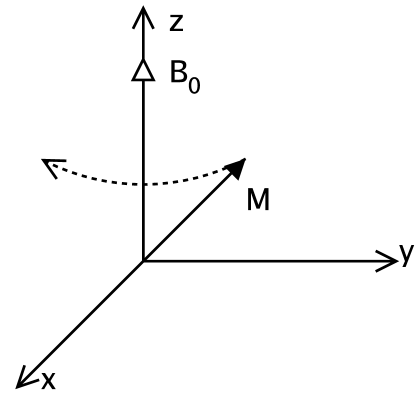
Figure 2.1: Precession when $\gamma>0$.

It is a well established fact that a magnetic dipole with moment perturbed from alignment with an external magnetic field will precess (Figure 2.1). This is the underlying physical basis for NMR. Precession is due to the torque $\vec{\mu}\times\vec{B_{0}}$ acting on the non-zero angular momentum of the nucleus [14, eq (7)]. The rate of precession is determined by the magnetogyric ratio (often called the gyromagnetic ratio), denoted by $\gamma$. This is the ratio (for a given nucleus) of magnetic moment to (spin) angular momentum, where $\hbar\vec{I}$ is the angular momentum of the nucleus. We write the magnetic moment in terms of $\gamma$ as

$$\vec{\mu}\equiv\gamma\,\hbar\,\vec{I}.$$ (2.5)

Table D.1 in Appendix D shows $\gamma$ for various common nuclei.

Mathematically we can express the precession the angular momentum for an ensemble of nuclei ($\vec{L}=\frac{1}{V}\sum_{n=1}^{N}\vec{l}_{n}$) by a differential equation, the torque being equal to the time rate of change of angular momentum as

$$\frac{d\,\vec{L}}{d\,t}=\vec{M}\times\vec{B}_{0}.$$ (2.6)

We can put this in the more useful form (since $\gamma\,\vec{L}=\vec{M}$)

$$\frac{d\,\vec{M}}{d\,t}=\gamma\vec{M}\times\vec{B}_{0}.$$ (2.7)

We note that when non-zero, the change in $\vec{M}$, $\frac{d\,\vec{M}}{d\,t}$, is always orthogonal to $\vec{M}$ as well as $\vec{B}_{0}$. This results in the circular “precession” about $\vec{B}_{0}$.

The solution to equation 2.7 is best carried out in spherical coordinates, with $\vec{B}_{0}$ oriented along the $z$ polar axis. Then we have

$$\frac{d\,\vec{M}}{d\,t}=-\gamma\,M\,B_{0}sin(\theta)\,\hat{\phi}.$$ (2.8)

Since the tip of $\vec{M}$ must traverse a “distance” $2\pi\,cos(\theta)\,M$ to make a full revolution, this corresponds to rotation about $\hat{z}$ at a rate $\frac{d\,\phi}{d\,t}=\omega_{0}=-\gamma\,B_{0}$ at a constant $\theta$. Note that in figure 2.1 the sense of rotation is left handed or clockwise about $\hat{z}$. This is because most nuclei of interest have a positive magnetogyric ratio , $\gamma>0$, although some nuclei posses $\gamma<0$.

In Cartesian coordinates the solution becomes

$$\vec{M}(t)=M_{0}[sin(\theta_{0})\,cos(\phi_{0}+\omega_{0}t)\,\hat{x}+sin(\theta_{0})\,sin(\phi_{0}+\omega_{0}t)\,\hat{y}+cos(\theta_{0})\,\hat{z}],$$ (2.9)

where $M_{0}$, $\theta_{0}$ and $\phi_{0}$ determine the initial magnitude and orientation of $\vec{M}$.

The frequency of precession

$$f=\frac{\omega_{0}}{2\pi}=-\frac{\gamma\,B_{0}}{2\pi}$$ (2.10)

is called the Larmor frequency.

2.4 Longitudinal and Transverse Components

Figure 2.2: Longitudinal and Transverse components of $\vec{M}$.

It is helpful to distinguish between longitudinal and transverse components of the magnetization (Figure 2.2). The longitudinal (oriented $\|$ to $\vec{B}_{0}$) component does not precess, while the transverse (oriented $\bot$ to $\vec{B}_{0}$) does precess. The longitudinal and transverse components of magnetization relax differently. We will discuss relaxation properties in chapter 4. Distinguishing between the longitudinal and transverse components of the magnetization will also be useful later when we discuss the distant dipolar field in Part II. The components are defined as

$$\vec{M}=\vec{M}_{\|}+\vec{M}_{\bot},$$ (2.11)

$$\vec{M}_{\|}\equiv M_{0}\,cos(\theta_{0})\,\hat{z},$$ (2.12)

and

$$\vec{M}_{\bot}\equiv M_{0}[sin(\theta_{0})\,cos(\omega_{0}t+\phi_{0})\,\hat{x}+sin(\theta_{0})\,sin(\omega_{0}t+\phi_{0})\,\hat{y}].$$ (2.13)

We can introduce an even further convenience, denoting the $\hat{x}$ component as the real part and the $\hat{y}$ component as the imaginary part of a complex scalar value, written as

$$\vec{M}_{\bot}\equiv Re(M_{\bot})\,\hat{x}+Im(M_{\bot})\,\hat{y}.$$ (2.14)

This gives us the form

$$M_{\bot}(t)=M_{0}sin(\theta_{0})\,e^{i\,(\omega_{0}t+\phi_{0})}.$$ (2.15)

Note that $\omega_{0}<0$ corresponds to clockwise or left-handed precession about $\hat{z}$ for nuclei with $\gamma>0$.

The longitudinal magnetization is always real and can be written as a real scalar

$$M_{\parallel}=M_{0}\,cos(\theta_{0}).$$

2.5 Rotating Frame

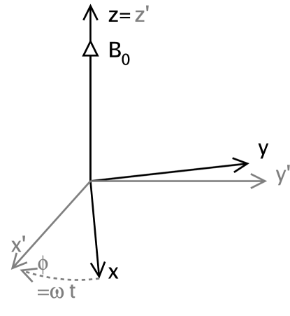
Figure 2.3: Rotating frame, $\omega_{0}<0$ and $t>0$.

Another helpful concept is the rotating frame [16]. We construct another Cartesian coordinate system, whose $z^{\prime}$ axis coincides with the laboratory frame $z$. The $x^{\prime}$ and $y^{\prime}$ axis rotates with angular frequency $\omega$. We show this in figure 2.3. In the rotating frame, if $\omega=\omega_{0}$, the magnetization will appear to stand still. The coordinate transformations are

$$\hat{x}^{\prime}=\hat{x}\,cos(\omega t)+\hat{y}\,sin(\omega t),$$ (2.16)

$$\hat{y}^{\prime}=\hat{y}\,cos(\omega t)-\hat{x}\,sin(\omega t)$$ (2.17)

and

$$\hat{z}^{\prime}=\hat{z}.$$ (2.18)

We can also define,

$$\Delta\omega_{0}\equiv\omega_{0}-\omega,$$ (2.19)

the angular frequency with which magnetization will precess in the rotating frame. This is sometimes called the resonance offset.

Related to equation (2.19) is the effective field $\vec{B}_{eff}$. This is a fictitious field (see figure 2.4) in the rotating frame such that

$$\vec{B}_{eff}=\frac{-\Delta\omega_{0}}{\gamma}\hat{z}.$$ (2.20)

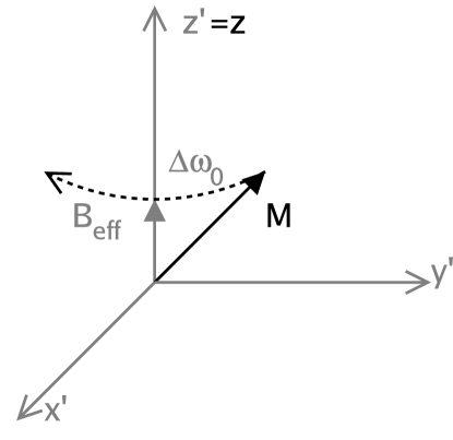
Figure 2.4: Effective field $\vec{B}_{eff}$ and resonance offset $\Delta\omega_{0}$ in the rotating frame.

By substituting (2.19) into (2.20) we get the relation

$$\vec{B}_{eff}=(B_{0}+\frac{\omega}{\gamma})\,\hat{z}.$$ (2.21)

Note that $B_{eff}=0$ when $\omega=\omega_{0}$. The rotating frame and effective field are extremely useful tools in understanding the dynamics of NMR and MRI experiments. The effective field can also include contributions from an applied radio frequency field (RF) discussed in section 3.1.

Chapter 3 OSCILLATING FIELD EFFECTS

3.1 RF Field

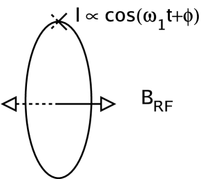
Figure 3.1: RF magnetic field $\vec{B}_{RF}$ due to a oscillating current in a conducting loop “transmit coil.”

The “resonance” in NMR and MRI refers to the response of nuclei to an applied oscillating magnetic field, called an “RF field” or “RF pulse”. For commonly achievable fields and nuclei the Larmor frequency falls within the 1-1000MHz frequency range, hence the term Radio Frequency or RF.

In general, the magnetic (and electric) field properties in an NMR experiment depend on the specific geometry of the RF coil, and sometimes the geometry and absorption properties of the sample. We will consider an idealized case of uniform RF fields and no absorption. The term “$B_{1}$ inhomogeneity” refers to the situation where the RF coil produces more RF magnetic field at one location than another. Some coils are designed with a homogeneous RF field in mind, such a solenoids or birdcages [17, 18, 19]. Others such as surface coils are not, and may require $B_{1}$ insensitive “adiabatic” pulses [20] for experiments sensitive to $B_{1}$ inhomogeneity.

We represent an applied RF magnetic field by its components. The magnetic field $B_{RF}$ at the center of a current loop (called the transmit coil) carrying an alternating current $I$ is perpendicular to the axis of the loop as in figure 3.1. We must break the field $B_{RF}$ into its counter-rotating components. The nucleus will only respond to a field rotating with the same sense and angular frequency near its own Larmor frequency. Mathematically we have

$$\vec{B}_{RF}=A\,cos(\omega_{1}t+\phi_{1})\,\hat{x},$$ (3.1)

$$\vec{B}_{RF}=\vec{B}_{1}+\vec{B^{\prime}}_{1},$$ (3.2)

$$\vec{B}_{1}=\frac{A}{2}\,cos(\omega_{1}t+\phi_{1})\,\hat{x}+\frac{A}{2}\,sin(\omega_{1}t+\phi_{1})\,\hat{y},$$ (3.3)

$$\vec{B^{\prime}}_{1}=\frac{A}{2}\,cos(\omega_{1}t+\phi_{1})\,\hat{x}-\frac{A}{2}\,sin(\omega_{1}t+\phi_{1})\,\hat{y}.$$ (3.4)

In the complex notation introduced in section 2.4 equation 2.15 we can write

$$B_{1}=\frac{A}{2}\,e^{i\,(\omega_{1}\,t+\phi_{1})},$$ (3.5)

$$B^{\prime}_{1}=\frac{A}{2}\,e^{i\,(-\omega_{1}\,t+\phi_{1})}.$$ (3.6)

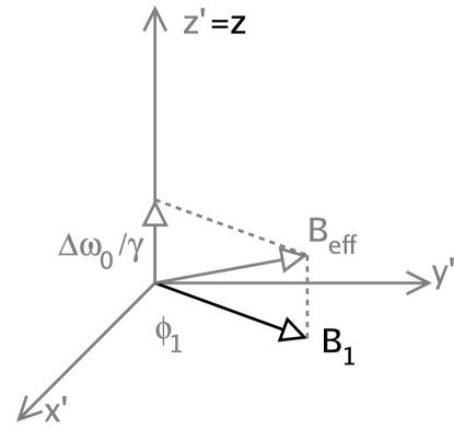
Figure 3.2: Effective field $\vec{B}_{eff}$ for $\omega_{1}=\omega$.

The component $B^{\prime}_{1}$ will in general have negligible effect on the system and can be ignored. Some coils produce a rotating field rather than a linear oscillating field, in which case no $B^{\prime}_{1}$ component is produced. An advantage of these coils is efficiency of utilization of RF power from the transmitter. In general the RF field amplitude $A$ is a function of time. The RF field can be turned on for periods of time, hence the term RF pulse.

An RF field with $\omega_{1}=\omega$ has a particularly simple representation in the rotating frame: it is a constant field that does not move. One can then add this $\vec{B}_{1}$ component to make a total $\vec{B}_{eff}$ in the rotating frame. If $\omega_{1}\neq\omega$ then the transverse component of $\vec{B}_{eff}$ (which is $\vec{B}_{1}$) will rotate with angular frequency $\Delta\omega_{1}=\omega_{1}-\omega$.

We can sum up these relations for $\vec{B}_{eff}$ in the rotating frame as

$$\vec{B}_{eff}=\frac{-\Delta\omega_{0}}{\gamma}\,\hat{z}+Re(B_{1}\,e^{i\,(\Delta\omega_{1}\,t+\phi_{1})})\,\hat{x}^{\prime}+Im(B_{1}\,e^{i\,(\Delta\omega_{1}\,t+\phi_{1})})\,\hat{y}^{\prime}.$$ (3.7)

$\phi_{1}$ is the “phase” of the RF field, $\phi_{1}=0$ corresponding to $B_{1}$ initially oriented along $\hat{x}^{\prime}$ and $\phi_{1}=\frac{\pi}{2}$ corresponding to $B_{1}$ initially oriented along $\hat{y}^{\prime}$. If the RF resonance offset $\Delta\omega_{1}=0$, then $\vec{B}_{eff}$ is constant in the rotating frame.

3.2 RF Pulse

Radio Frequency (RF) pulses are the principal workhorses of NMR and MRI. Magnetization precesses about the effective field $\vec{B}_{eff}$ in the rotating frame. For $\Delta\omega_{1}=0$, $\vec{B}_{eff}=\vec{B}_{1}$ and lies in the transverse plane. Turning on or off, or varying the amplitude $B_{1}$ of the RF field by applying an “RF Pulse” is the principal activity in any NMR experiment.

3.2.1 90° Pulse

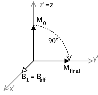
Figure 3.3: $90^{\circ}$ RF Pulse

Figure 3.3 shows an RF pulse that moves $\vec{M}$ from its equilibrium position $\vec{M}_{0}$ aligned with the $z$ axis into the transverse plane such that $\gamma\,B_{1}\tau=\frac{\pi}{2}$. $\tau$ is the duration of the pulse. A more complicated but equivalent form is

$$\gamma\int_{0}^{\tau}\,B_{1}(t)\,dt=\frac{\pi}{2},$$ (3.8)

which allows for the amplitude of $B_{1}$ and hence the precession rate of $\vec{M}$ about the $B_{1}$ field to vary in time. A 90° RF pulse acting on equilibrium magnetization is often called an excitation pulse.

3.2.2 180° Pulse

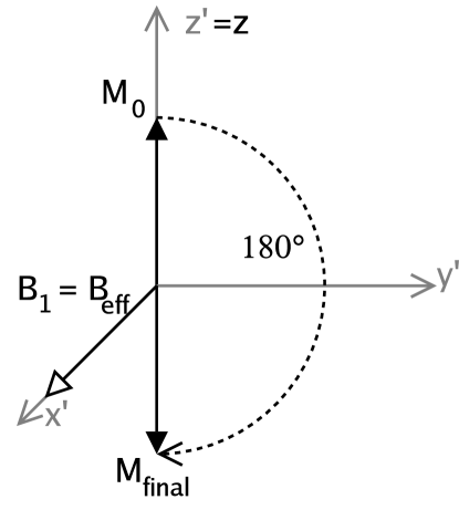
Figure 3.4: $180^{\circ}$ RF Pulse

A 180° pulse inverts the magnetization from its equilibrium value. It has twice the “area,” as defined in equation 3.8, as a 90° pulse. A 180° pulse acting on equilibrium magnetization is often called an inversion pulse.

3.2.3 Off-Resonance Pulse

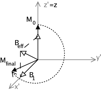
Figure 3.5: Same $180^{\circ}$ RF Pulse as figure 3.4, but off-resonance.

In the prior examples we have assumed that the RF field $B_{1}$ is on resonance. If this is not true $B_{eff}$ will not lie in the transverse plane. The effect of an off-resonance $B_{1}$ field is almost always to reduce the total rotation angle compared to one on-resonance for a given pulse. This can be seen as follows. We will assume the same constant magnitude of $B_{1}$ field and duration as in figure 3.4. A pulse with constant $B_{1}$ is also known as a “hard pulse”. On-resonance the pulse is a $180^{\circ}$pulse. Consider $\frac{\gamma\,B_{1}}{2\pi}=500Hz$. This form is a convenient measure of $B_{1}$ amplitude and is often shortened to $B_{1}=500Hz$. In this case for a $180^{\circ}$pulse we need $\tau=1ms$. If the nuclei of interest are $500Hz$ off resonance we have the following situation seen in figure 3.5. The pulse gives less than $90^{\circ}$ of rotation, and has a phase offset as well.

3.3 Pulse Bandwidth

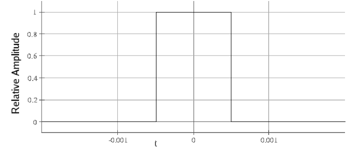
Figure 3.6: Hard pulse envelope, duration is $1ms$.

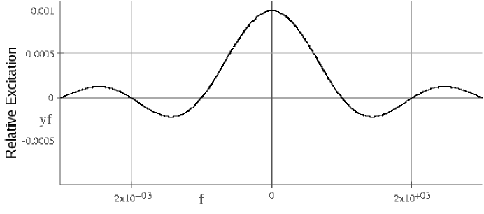
Figure 3.7: Fourier transform (approximate excitation profile) of the hard pulse in figure 3.6. The bandwidth is approximately $1200Hz$.

The “bandwidth” of the pulse is defined as the total frequency range for which the rotation angle is above half the on-resonance value. In section 3.2.3 the pulse has a bandwidth of about $1200Hz$ or $1.2kHz$. Bandwidth in inversely proportional to $\tau$ and depends on the shape of the pulse.

To find the bandwidth of a pulse (see figure 3.6) one needs to solve the Bloch equations for the specific pulse shape for a number of resonance offsets. One can also perform an experiment to determine the performance of the pulse for excitation (or inversion), this is called the excitation (or inversion) profile. The Fourier transform of the RF pulse envelope (see figure 3.7) gives a good approximation to the excitation profile. The excitation profile shows the relative rotation angle achieved versus the resonance offset. The approximate pulse bandwidth is the full-width-half-max of this approximate excitation profile.

3.4 Free Induction Decay

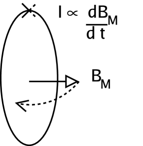
Figure 3.8: Detecting precessing magnetization by induced current in receiver coil.

Following a 90° pulse, the magnetization is entirely in the transverse plane, and continues to precess in the transverse plane in the laboratory frame (since the RF field is zero after the pulse). In the rotating frame the magnetization will precess according to its resonance offset $\Delta\omega_{0}$.

The magnetic field associated with the precessing magnetization can be detected by its ability to induce a current in a nearby placed coil, called the receiver coil. The transmit and receiver coils can be the same or different. The current induced in the receiver coil is amplified, mixed with a local oscillator down to the audio frequency range, and digitized.

One can equate the local oscillator frequency of the receiver with the frequency of rotation of the rotating frame. The output of the mixer will then oscillate at the frequency of the resonance offset. Shown in figure 3.9 is an example oscilloscope trace from an early pulsed NMR experiment.

The signal is called the “Free Induction Decay” or FID. The “Decay” comes from relaxation processes, which we will discuss in section 4.

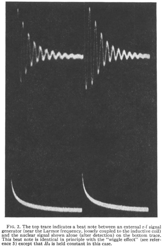
Figure 3.9: Free induction decay (FID) for two excitations displayed on an analog oscilloscope. From reference [22], Copyright 1950 by The American Physical Society, used with permission.

3.4.1 Quadrature Detection

Note that there will be an ambiguity as to the sign of the offset $\Delta\omega_{0}$ unless more information is obtained. This is achieved by quadrature detection. The idea is to get information about both the real and imaginary components of the precessing magnetization. This can be done in several ways. Originally it was done in an analog manner by having two reference oscillators (or on oscillator and a phase shifter) and demodulating two signals, the phase of one shifted by $90^{\circ}$ with respect to the other [23, 24, sec. 6.4]. In digital systems it can be done in a number of ways by oversampling and digital signal processing.

3.4.2 NMR Spectrum

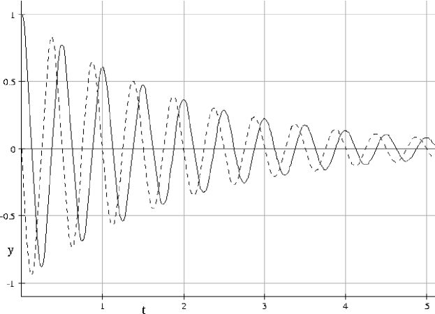
(a) Complex FID.

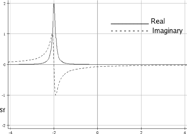
(b) Spectrum

Figure 3.10: (a) Real and Imaginary part of the FID. (b) Complex Fourier Transform of the FID yields the complex NMR spectrum. Usually only the real part of the spectrum, after phase correction, is shown.

The complex Fourier transform of the FID yields the NMR Spectrum [25, 26]. See figure 3.10 for a simple simulated example. For the real part of the spectrum to be Lorentzian it is often necessary to phase correct the spectrum [27, 28, sec. 5.1]. Originally NMR spectra were not obtained in this way, rather the RF frequency (or $B_{0}$ field strength at constant RF frequency) was swept across the range of interest. These so-called Absorption/Induction methods have been shown to yield equivalent information to the Fourier method [29], however the Fourier method has many signal-to-noise and speed of measurement advantages and is almost universally used in modern NMR spectrometers. The principal activity in NMR spectroscopy is the identification of peaks of differing chemical shifts (see section 4.4). Many other parameters can also be measured such as relaxation rates (chapter 4) and diffusion (chapter 7).

Chapter 4 RELAXATION

Relaxation is the name given to processes in which magnetization decays or returns to equilibrium. There are two principal processes of interest, still named by their original designations and symbols [30].

4.1 Longitudinal Relaxation, $T_{1}$

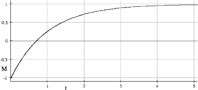
Figure 4.1: Recovery of inverted magnetization by $T_{1}$ relaxation as described by equation 4.3. $T_{1}=1$ unit.

Longitudinal relaxation, also called spin-lattice relaxation, using symbol $T_{1}$, describes the time scale at which magnetization returns to thermal equilibrium, $M_{0}$, after being perturbed away from equilibrium, such as by an RF pulse. Its effects are described by the following equation for the recovery of the longitudinal magnetization

$$M_{\|}(t)=M_{0}-(M_{0}-M_{\|initial})\,e^{-t/T_{1}},$$ (4.1)

which is the solution to the differential equation

$$\frac{dM_{\parallel}}{dt}=\frac{M_{0}-M_{\parallel}}{T_{1}}.$$ (4.2)

An important approximation is that $M_{\|}(t)\approx M_{0}$ after a period $t=5\times T_{1}$. This can also be seen in Figure 4.1.

The term spin-lattice relaxation refers to transfer of energy from the nuclear spins composing the macroscopic magnetization to the “lattice,” a catch-all term referring to all other possible energy levels in the system. The details of spin-lattice relaxation are beyond the scope of this dissertation. Suffice it to say that in liquids, the main mechanism of longitudinal relaxation is RF fields from nearby spins causing stimulated transitions so that equilibrium is attained. Spontaneous emission processes at NMR frequencies are entirely negligible [31]. Information can be found in references [30, 32, 33, 34, 35, 36, 37, 9].

4.1.1 Repetition and Recovery

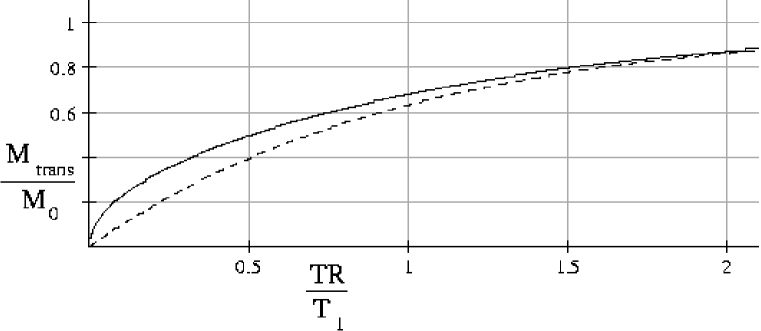
Figure 4.2: Transverse magnetization obtained in the steady state by exciting at the Ernst angle $\theta_{E}=arccos(e^{-\frac{TR}{T_{1}}})$ ——– vs. exciting at $90^{\circ}$ - - - -.

In many NMR and MRI experiments the system is re-exited before full relaxation (before waiting $5\times T_{1}$) has occurred. Often this is to speed up the total time necessary to make an image in MRI or to acquire a 2d NMR spectrum. The time between multiple excitations is called the “repetition time” and denoted by $TR$. There is an optimum RF excitation pulse to maximize the signal given a specific $TR$ and $T_{1}$ which is called the Ernst angle [38, p. 155]. To find the Ernst angle we find the steady state longitudinal magnetization after a large number of repetitions. We solve the equation

$$M_{\|SS}=M_{0}-[M_{0}-M_{\|SS}cos(\theta)]\,e^{-t/T_{1}}$$ (4.3)

formed by substituting $M_{\|}=M_{\|SS}$ and $M_{\|initial}=M_{\|SS}cos(\theta)$ into equation 4.3. The solution is

$$M_{\|SS}=M_{0}\frac{e^{\frac{TR}{T_{1}}}-1}{e^{\frac{TR}{T_{1}}}-cos(\theta)}.$$ (4.4)

The transverse magnetization immediately after excitation will be

$$M_{\bot SS}=M_{\|SS}\,sin(\theta).$$ (4.5)

We can then find the excitation angle at which the transverse magnetization becomes maximum, consistent with the steady-state longitudinal magnetization. We set the result equal to zero, i.e.

$$\frac{\partial M_{\bot SS}}{\partial\theta}=0=M_{0}\frac{e^{\frac{TR}{T_{1}}}(e^{\frac{TR}{T_{1}}}-1)\,cos(\theta)-(e^{\frac{TR}{T_{1}}}-1)}{[e^{\frac{TR}{T_{1}}}-cos(\theta)]^{2}},$$ (4.6)

which has the solution

$$cos(\theta_{E})=e^{-\frac{TR}{T_{1}}}.$$ (4.7)

When $TR\geq 5\times T_{1}$ we have $cos(\theta_{E})\approx 1$ and $\theta_{E}\approx 90^{\circ}$ as expected. Figure 4.2 shows a comparison of the signal using the Ernst angle vs. using $90^{\circ}$ as a function of $\frac{TR}{T_{1}}$.

4.2 Transverse Relaxation, $T_{2}$

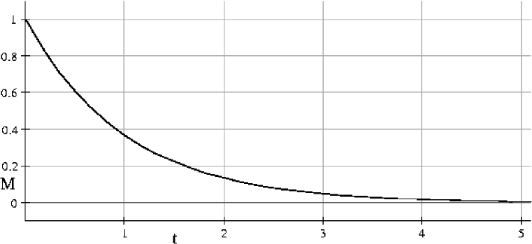
Figure 4.3: $T_{2}$ decay of transverse magnetization as described by equation 4.8. $T_{2}=1$ unit.

Transverse relaxation refers to the decay of transverse magnetization with time. It is called spin-spin relaxation and is designated by the symbol $T_{2}$. Phenomenologically it can be described by the equation

$$M_{\bot}(t)=M_{\bot initial}\,e^{-t/T_{2}}$$ (4.8)

in which the initial transverse magnetization decays exponentially with time. This is the solution to the differential equation

$$\frac{dM_{\perp}}{dt}=-\frac{M_{\perp}}{T_{2}}.$$ (4.9)

Figure 4.3 shows the $T_{2}$ decay curve where $T_{2}$ is one time unit in magnitude.

The term spin-spin relaxation originates from the mechanism whereby the field from other nuclei and nearby molecules, atoms, or ions is a random function of time, and causes a slight change in phase of a given nuclear moment’s precession. These random phase variations accumulate over time, causing a reduction in the net macroscopic transverse magnetization.

The details of transverse relaxation mechanisms are beyond the scope of this dissertation; the reader is referred to references [30, 32, 34, 39, 35, 36, 9].

4.3 Field Inhomogeneity, $T_{2}^{\dagger}$ and $T_{2}^{*}$

There is another decay process analogous to transverse $T_{2}$ relaxation. It is due to variations in the local magnetic field, but over macroscopic distances and in a temporally deterministic (temporally non-random) manner. Variation in the applied field $B_{0}$ is usually called “$B_{0}$ inhomogeneity” while susceptibility induced variations go by the name “sample inhomogeneity” or “susceptibility gradients.”

The accumulated random phase variations are assumed to cause an exponential decay $T_{2}^{\dagger}$ . We combine the microscopic $T_{2}$ and macroscopic $T_{2}^{\dagger}$ decay process into one decay constant $T_{2}^{*}$ with

$$\frac{1}{T_{2}^{*}}=\frac{1}{T_{2}}+\frac{1}{T_{2}^{\dagger}}.$$ (4.10)

The transverse magnetization will then be described by the equation

$$M_{\bot}(t)=M_{\bot initial}\,e^{-t/T_{2}^{*}}.$$ (4.11)

We will talk about $B_{0}$ and sample inhomogeneity more in section 9.

4.4 Chemical Shift

In addition to the applied field, field inhomogeneity, and susceptibility fields, each nuclear spin experiences a “local field.” This is due to the field of electrons and nuclei in the rest of the molecule containing it, and fields from nearby molecules. This field is constantly changing due to translational, vibrational, and rotational motion. It is the fluctuating component of this local field that leads to relaxation [30]. The time average component leads to a shift in the Larmor frequency, called the chemical shift [41].

There are two components of the shift, a dominant field proportional shift (due to diamagnetic effects), and another usually smaller absolute shift due to “J-coupling” through bonds to other paramagnetic nuclei in the molecule [42, 43, 44].

The field proportionality constant of the field dependent chemical shift is often denoted by the symbol $\sigma$, and can be thought of as the normalized resonance offset relative to a “reference” Larmor frequency $\omega$. This is written

$$\sigma\equiv\frac{\omega_{0}-\omega}{\omega}.$$ (4.12)

$\sigma$ is dimensionless and is almost always reported in units of $10^{-6}$ or “parts per million” (ppm).

The chemical shift gives information about local chemical bond geometry and average motion. It is the principal parameter of interest for determining chemical structure using modern NMR spectroscopy [45]. A more detailed discussion of the origin of chemical shift can be found in [9, section 7.7].

Chapter 5 SPIN-ECHO

The spin-echo is another key concept of NMR and MRI. First demonstrated by E. L. Hahn [41], spin-echoes continue to be utilized in many NMR and MRI experiments. The spin-echo is a way of refocusing (or re-phasing) the effects of temporally static field inhomogeneities (see section 4.3).

A spin-echo consists of a 90° pulse to excite transverse magnetization followed by a 180° pulse, shown in figure 5.1. The effect of the 180° pulse is to invert the phase of the transverse magnetization. Any phase acquired due to field inhomogeneities or gradients (see section 6) during the $TE/2$ time period before the 180° pulse is canceled by the phase acquired during the $TE/2$ time period after the 180° pulse.

The envelope of a spin-echo free induction decay (FID) (not counting off resonance oscillation, such as chemical shift) is

$$M_{\bot}(t)=M_{\bot initial}e^{-t/T_{2}}e^{-|t-TE|/T_{2}^{\dagger}}.$$ (5.1)

$TE$ is called the echo-time. Note that the build (before $\frac{TE}{2}$) and decay (after $\frac{TE}{2}$) sides of the FID are not symmetric in the presence of $T_{2}$ decay.

It is possible to use multiple 180° pulses (spaced $TE$ apart) and refocus multiple echoes. This is sometimes called a CP sequence after Carr and Purcell [46], who originally used such a sequence to examine the effects of diffusion (see section 7) and $T_{2}$ relaxation. Modification of the phase of the RF pulses (where the inversion pulses are shifted by 90° in phase) is called CPMG sequence, from Carr-Purcell-Meiboom-Gill [47]. A CPMG sequence has the desirable property of being less sensitive to pulse amplitude errors than a CP sequence, especially for the even echoes. This latter property is sometimes called “even echo re-phasing.”

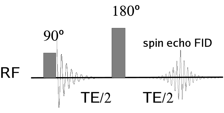
Figure 5.1: Spin-echo pulse sequence.

Chapter 6 GRADIENTS

Magnetic field gradients are a useful tool in NMR spectroscopy for destroying unwanted signals and introducing diffusion weighting (see chapter 7). Gradients are required for MRI.

A gradient is produced by a secondary set of magnetic coils, designed so that the field varies linearly with position along the direction of the gradient [48]. An $x$ gradient field can be represented by the equation

$$\Delta\vec{B}(x)=G_{x}x\,\hat{z}.$$ (6.1)

Note that the direction of the gradient refers to the direction along which the gradient strength varies, not the direction of the field. MRI instruments usually possess three gradient coils, to produce orthogonal $x$, $y$, and $z$ gradients. These can be linearly combined into an arbitrary gradient direction $\hat{s}$.

Applying a gradient causes the magnetization to twist into a helix along the direction of the gradient. The longer the gradient is applied, the more twisted the transverse magnetization becomes. The resulting NMR signal, when the magnetization is in a twisted state, is greatly reduced when there are many twists across the sample. This is sometimes called “crushing” or “spoiling” the transverse magnetization.

6.1 Pulsed Gradients

Gradient hardware is designed so that it can deliver pulses, much like the RF coil and transmitter discussed earlier. In modern instruments the gradient amplitude can be controlled digitally so that the amplitude of the gradient can be made a function of time. Figure 6.1 shows the transverse magnetization along an arbitrary gradient direction $\hat{s}$ after a gradient pulse.

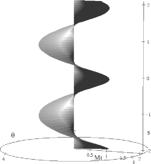
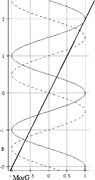
Figure 6.1: Transverse magnetization helix after gradient pulse along arbitrary direction $\hat{s}$. The Gradient $G_{s}$ is shown as heavy line in the component graph, $M_{x}$ is a normal line and $M_{y}$ is dashed.

6.1.1 Pulse Sequence

A series of RF and gradient pulses, interspersed with delays and acquisition periods, is called a pulse sequence. We have already seen an example (without gradients) in figure5.1.

6.2 Secular Approximation of Quasi-static Fields

In the presence of a large applied magnetic field, small additional static (or slowly varying) fields such as gradients can be treated as a perturbation. We can look at the effect of a gradient on the Larmor frequency first with the gradient field $\Delta\vec{B}(x)=G_{x}x\,\hat{z}$ oriented in the same direction as the applied field $\vec{B}_{0}$=$B_{0}\hat{z}$, and then with the gradient field oriented orthogonally $\Delta\vec{B}(x)=G_{x}x\,\hat{y}$.

When the gradient field is oriented parallel to $\vec{B}_{0}$ we have

$$\vec{B}=B_{0}\hat{z}+G_{x}x\,\hat{z}.$$ (6.2)

The field magnitude is

$$B=B_{0}+G_{x}x,$$ (6.3)

causing a first order change in the Larmor frequency

$$\Delta f=\frac{-\gamma}{2\pi}(G_{x}x).$$ (6.4)

When the gradient field is oriented orthogonal to the large applied field we have

$$\vec{B}=B_{0}\hat{z}+G_{x}x\,\hat{y}.$$ (6.5)

The field magnitude is then

$$B=\sqrt{B_{0}^{2}+(G_{x}x)^{2}},$$ (6.6)

which we can expand in a Taylor’s series to

$$B\approx B_{0}+\frac{(G_{x}x)^{2}}{2\,B_{0}}^{\prime}$$ (6.7)

which yields

$$\Delta f\approx\frac{-\gamma}{4\pi}\frac{(G_{x}x)^{2}}{B_{0}}.$$ (6.8)

If we set values for $B_{0}=4.7T$ and $G_{x}=200\frac{mT}{m}$ with $x=1cm$ in the parallel case we have $|\Delta f|=85.15kHz$ and in the orthogonal case $|\Delta f|=18.12Hz$, which is more than 3 orders of magnitude smaller. Most susceptibility gradients and inhomogeneities are much smaller than $200\frac{mT}{m}$, and if their field orientations are not along $\vec{B}_{0}$, they can safely be ignored.

The above approximation of ignoring field components perpendicular to the static field is called the secular approximation or taking the secular component of the field. We will address the secular component of fields that include a rotating component (are rapidly varying) in section 11.3 and appendix A.4.

Chapter 7 DIFFUSION

In many NMR and most MRI experiments the sample of interest is a liquid or composed of liquids in biological compartments. There are many fortuitous properties of a liquid sample that make NMR easier than on a solid sample. When the nucleus of interest is in a liquid, the random motion of molecules causes an averaging effect on the fields due to other nearby nuclei and molecules. This contributes to so called “motional narrowing” giving liquids much narrower spectral lines than solids. For details see references [30, sec. X] [49] [9, ch. 15] [36, ch. X] and [50, sec. 5.12].

We can think of a molecule in a liquid as taking a “random walk” in three dimensions. Assuming no macroscopic flow (or convection), the motion will be mainly due to thermal kinetic energy and collisions with other molecules. If the sample has no barriers, and is a normal liquid (not a liquid crystal), the motion will be isotropic, meaning that motion in any direction is equally probable.

7.1 Fick’s Laws

Diffusion of a scalar field $c(\vec{r},\,t)$ can be described by Fick’s first law [51]

$$\vec{J}(\vec{r},\,t)=-\mathbf{D}\nabla c(\vec{r},\,t).$$ (7.1)

$\vec{J}$ is the flux of a given substance (or field), $c(\vec{r},\,t)$, is the concentration (or field amplitude), and $\mathbf{D}$ is the diffusion tensor (discussed in section 7.1.2). In simple terms this equation says that there is a “flow” from high concentration to low concentration. Heat flow obeys a diffusion equation and so does the motion of molecules in a liquid (if there is no macroscopic flow or convection). We can combine this with the continuity equation

$$\frac{\partial c(\vec{r},\,t)}{\partial t}=-\nabla\cdot\vec{J}(\vec{r},\,t).$$ (7.2)

Equation 7.2 says that the time rate of change in concentration must be equal to the divergence of the flux (what goes into a small volume either goes out or increases the concentration). Fick’s second law, also called the diffusion equation, is therefore

$$\frac{\partial c(\vec{r},\,t)}{\partial t}=\nabla\cdot\mathbf{D}\nabla c(\vec{r},\,t).$$ (7.3)

The diffusion equation reduces to

$$\frac{\partial c(\vec{r},\,t)}{\partial t}=D\nabla^{2}c(\vec{r},\,t),$$ (7.4)

where D is a constant, for isotropic diffusion.

7.1.1 Diffusion in 1d

We will first consider diffusion in one dimension. The probability that a molecule $n$ will be found a distance $x$ from its starting point is given by

$$P(x_{n},\,t)=\frac{e^{-\frac{x_{n}^{2}}{4\,D_{x}t}}}{\sqrt{4\,\pi\,D_{x}t}}.$$ (7.5)

Equation 7.5 says that the probability is normally distributed (as expected from a large number of random collisions and motions), with the variance $2\,D_{x}t$ increasing linearly with time.

It also is the solution to the 1d diffusion equation

$$\frac{\partial P(x_{n},\,t)}{\partial t}=D_{x}\,\frac{\partial^{2}P(x_{n},\,t)}{\partial x^{2}}.$$ (7.6)

$D_{x}$ is the diffusion coefficient and has units of $[\frac{m^{2}}{s}]$. At room temperature the diffusion coefficient of water (in water) is $2.2\times 10^{-9}\frac{m^{2}}{s}$. An example is shown in figure 7.1. Notice that at 100 seconds there is still only a small probability of finding the molecule greater than 1mm from its starting point. This is why stirring is much more effective than diffusion for mixing at short times.

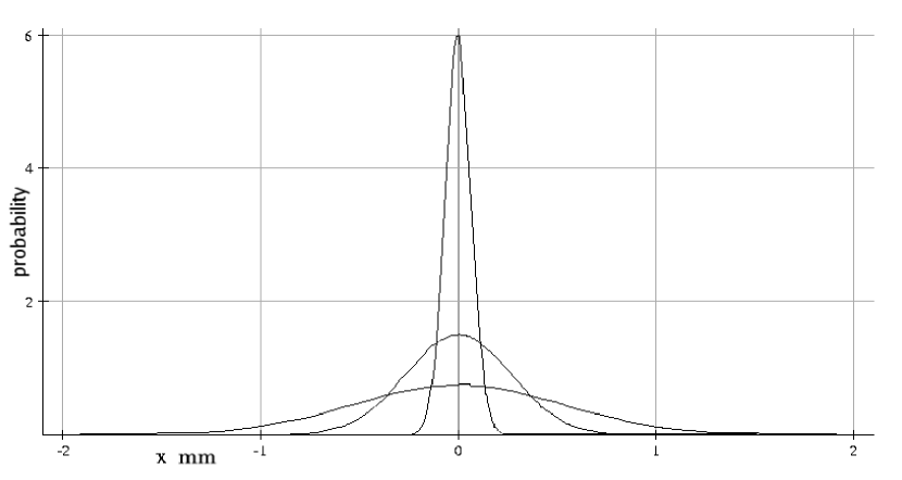
Figure 7.1: Diffusion of water in water (self-diffusion) at 1s, 10s, and 100s.

When we have a large number of identical molecules we can think of molecules starting in a small region distributing themselves into a larger region. We cannot predict where an individual molecule will go, but we do know on average how they will be distributed. This is also called an ergodic average.

7.1.2 Diffusion in 3d

We can treat the problem of diffusion in three dimensions separably, that is as three one dimensional problems. In this case we can consider the possibility of the diffusion coefficients in each direction being different. This is not the case for most pure liquids, but is often the case in biological tissues where barriers and restriction in compartments cause the “apparent diffusion coefficient” to depend on direction. In general, the apparent diffusion in a biological sample coefficient could be more complicated, depending on the exact direction of interest.

In the 3d case the probability distribution is

$$P(x_{n},\,y_{n},\,z_{n},\,t)=\frac{e^{-\frac{x_{n}^{2}}{4\,D_{x}t}}}{\sqrt{4\,\pi\,D_{x}t}}\frac{e^{-\frac{y_{n}^{2}}{4\,D_{x}t}}}{\sqrt{4\,\pi\,D_{y}t}}\frac{e^{-\frac{z_{n}^{2}}{4\,D_{x}t}}}{\sqrt{4\,\pi\,D_{z}t}}.$$ (7.7)

A useful extension is to allow the axes, while still orthogonal, to be rotated in an arbitrary direction. This leads to the so called “diffusion tensor”[52],

$$\mathbf{D}=\left(\begin{array}[]{ccc}D_{xx}&D_{xy}&D_{xz}\\ D_{yx}&D_{yy}&D_{yz}\\ D_{zx}&D_{zy}&D_{zz}\end{array}\right).$$ (7.8)

We define the reciprocal diffusion tensor as

$$\mathbf{D}_{rec}=\left(\begin{array}[]{ccc}D_{xx}^{-1}&D_{xy}^{-1}&D_{xz}^{-1}\\ D_{yx}^{-1}&D_{yy}^{-1}&D_{yz}^{-1}\\ D_{zx}^{-1}&D_{zy}^{-1}&D_{zz}^{-1}\end{array}\right).$$ (7.9)

The probability distribution (dropping the $n$ subscript) becomes

$$P(\vec{r},\,t)=\frac{e^{-\frac{\vec{r}^{T}\mathbf{D}_{rec}\vec{r}}{4\,t}}}{\sqrt{(4\,\pi\,t)^{3}\left|\mathbf{D}\right|}},$$ (7.10)

where $T$ denotes the transpose operation and $\left|\mathbf{D}\right|$ is the determinant. When diffusion is isotropic $\mathbf{D}$ becomes a scalar $D$ and equation 7.11 becomes

$$P(r,\,t)=\frac{e^{-\frac{r^{2}}{4\,D\,t}}}{\sqrt{(4\,\pi\,D\,t)^{3}}}.$$ (7.11)

Both solutions obey the differential equation,

$$\frac{\partial P(\vec{r},\,t)}{\partial t}=\nabla\cdot\mathbf{D}\nabla P(\vec{r},\,t),$$ (7.12)

which reduces to

$$\frac{\partial P(r,\,t)}{\partial t}=D\,\nabla^{2}P(r,\,t)$$ (7.13)

for the isotropic case.

7.2 Self-Diffusion in water

In NMR and MRI we are often interested in self-diffusion of water. This is the diffusion of water molecules in a solution that is composed of other water molecules. In order for this diffusion to be detected we must “label” the water molecules in some manner. The most convenient way to label the water molecules is by using a gradient or RF pulse to change the amplitude or orientation of the nuclear magnetization of the ${}^{1}H$ molecules. We can now talk about the diffusion of the magnetization itself.

Since magnetization is a vector quantity we have to modify the diffusion equation to operate on a vector field. This is to say that diffusion operates on each of the components of the magnetization. The equation for magnetization with (isotropic) diffusion in the rotating frame is

$$\frac{\partial\vec{M}}{\partial t}=D\nabla^{2}\vec{M}.$$ (7.14)

7.2.1 Diffusion Weighting with Gradients

Application of gradients during an NMR or MRI experiment can cause additional attenuation of the signal when there is significant diffusion. In early experiments [46] this was recognized as a confounding factor in measuring $T_{2}$. Later, NMR and MRI measurement of the diffusion properties of solutions and biological samples developed into a rich subfield in itself [53, 52, 51, 54].

When no gradients are present, diffusion will not explicitly affect the NMR signal. When a gradient is applied, the phase of spins in the transverse plane is altered as a function of position along the direction of the gradient (there is also dependence on gradient strength and the duration). If there is diffusion along the gradient direction, then spins labeled with one phase will move into regions of spins having a different phase. This causes a net reduction in the macroscopic transverse magnetization, and detected achievable signal. A pulse sequence where the signal responds in a known manner to diffusion is called “diffusion weighted.” It is also possible to have diffusion weighting due to diffusing longitudinal magnetization.

We show examples and signal equations of sequences with diffusion weighting in section 10.1 and 10.2.

Chapter 8 BLOCH EQUATIONS

The Bloch equations are a set of coupled differential equations that describe the behavior of the macroscopic magnetization [14, 36, ch. III. sec. II.]. The equations can account for the effects of precession, relaxation, field inhomogeneity, and RF pulses that we have already seen in previous sections. If one considers the magnetization as a function of space as well as time, we can include the effects of gradients and diffusion [55, 51].

8.1 Vector Bloch Equation

The vector Bloch equation in the notation introduced in the previous sections is

$$\frac{d\vec{M}}{dt}=\gamma\,\vec{M}\times\vec{B}+\frac{(\vec{M}_{0}-\vec{M}_{\|})}{T_{1}}-\frac{\vec{M}_{\perp}}{T_{2}}+\nabla\cdot\mathbf{D}\nabla\vec{M}.$$ (8.1)

$\vec{B}$ is assumed to include all applied fields as well as the field $\bigtriangleup\vec{B}$ due to $\vec{B}_{0}$ inhomogeneity and susceptibility effects. All fields could be written as functions of $\vec{r}$ if we wish to capture inhomogeneity and gradient effects. $\vec{B}_{1}$and $\vec{G}_{s}$are also functions of $t$ as determined by the pulse sequence. We write all this as

$$\vec{B}=\vec{B}_{0}+\vec{B}_{1}+\vec{G}_{s}s+\bigtriangleup\vec{B}.$$ (8.2)

In general $T_{1}$, $T_{2}$ and $\mathbf{D}$ could be functions of $\vec{r}$ as well. We can transform to the rotating frame by replacing $\vec{B}_{0}$ with $\frac{\Delta\omega_{0}}{\gamma}\hat{z}$ and make sure that the frequency of $\vec{B}_{1}$ is offset accordingly.

8.2 Longitudinal and Transverse Bloch Equations

We can break the single vector equation into its longitudinal and transverse components. We will use the complex notation for the transverse components. The equation for the longitudinal component is

$$\frac{dM_{\parallel}}{dt}=\gamma\,[\vec{M}\times\vec{B}]_{\parallel}+\frac{(M_{0}-M_{\parallel})}{T_{1}}+\nabla\cdot\mathbf{D}\nabla M_{\parallel}.$$ (8.3)

Noting that $B_{\perp}=B_{1}$, the term $\gamma\,[\vec{M}\times\vec{B}]_{\parallel}$can be expanded (see appendix A.2) to yield,

$$\frac{dM_{\parallel}}{dt}=\frac{i\gamma}{2}(M_{\perp}B_{1}^{*}-M_{\perp}^{*}B_{1})+\frac{(M_{0}-M_{\parallel})}{T_{1}}+\nabla\cdot\mathbf{D}\nabla M_{\parallel}.$$ (8.4)

For the transverse component we have

$$\frac{dM_{\perp}}{dt}=\gamma\,[\vec{M}\times\vec{B}]_{\perp}-\frac{M_{\perp}}{T_{2}}+\nabla\cdot\mathbf{D}\nabla M_{\perp},$$ (8.5)

and on expanding the cross product

$$\frac{dM_{\perp}}{dt}=i\,\gamma\,(M_{\parallel}B_{1}-M_{\perp}B_{\parallel})-\frac{M_{\perp}}{T_{2}}+\nabla\cdot\mathbf{D}\nabla M_{\perp}$$ (8.6)

with

$$B_{\parallel}=B_{0}+G\,s+\bigtriangleup B.$$

One replaces $B_{0}$ with $\frac{-\Delta\omega_{0}}{\gamma}$ in the rotating frame. Note that in the above equations only the $B_{1}$ RF field couples the transverse and longitudinal magnetization. We will see in part II that there is another process called “radiation dampening” that can achieve this as well.

Chapter 9 SHIMMING

Most NMR and MRI experiments rely on having a constant large applied magnetic field over the volume of the sample. The NMR signal is the average of the magnetization from each small volume element of the sample. If the applied field varies over the sample, the magnetization from different regions of the sample will get out of phase. This leads to reduction in the overall signal from the sample and broadening of spectral lines. We discussed this effect in section 4.3.

The $B_{0}$ field in an NMR spectrometer or MRI system is created by a large magnet, in most cases a superconducting electromagnet [56, 57, 58]. Magnets designed for NMR and MRI have very stringent requirements for homogeneity. In high resolution spectroscopy it is often desired to get homogeneity of the order of 0.1Hz in a field of 600MHz over a 1cm diameter volume. This is less than one part per billion. Homogeneity requirements in imaging are much less stringent, but typically are required over much larger volumes. One would usually like to achieve 10Hz over a 20cm diameter volume at a field strength of 1.5T, or approximately 0.1 parts per million (ppm).

Because of imperfections in the magnet, inherent in the design, due to manufacturing tolerances, or changes with age and use, all NMR and MRI magnets have additional smaller magnets called shims to adjust the homogeneity [59, 60]. Often there are two or three sets of shims, “steel,” “superconducting,” and “room temperature.” Steel shims are adjusted as part of the charging procedure after the main magnet is brought up to field. They consist of either a set of steel slugs or bands that are placed with the help of field mapping and fitting software. Superconducting shims are secondary coils wound within the cryostat. They are adjusted by altering their currents after the magnet is charged and stabilized, and can also be adjusted as part of maintenance.

In addition to imperfections in the magnet, shims compensate for susceptibility-induced fields, which vary from sample to sample (or patient to patient in MRI). Room temperature shims are electromagnetic coils. They are adjusted on a per sample basis. Often this is by means of an automated “pre-scan” procedure in clinical imaging. Often, in order to achieve narrow line-widths in NMR spectroscopy, manual shimming is necessary, which can be time consuming for the less experienced user.

Chapter 10 EXAMPLE PULSE SEQUENCES

In the following sections the Bloch equations are used to solve for the magnetization and signal for pulse sequences relevant to this dissertation.

10.1 Stejskal-Tanner Sequence

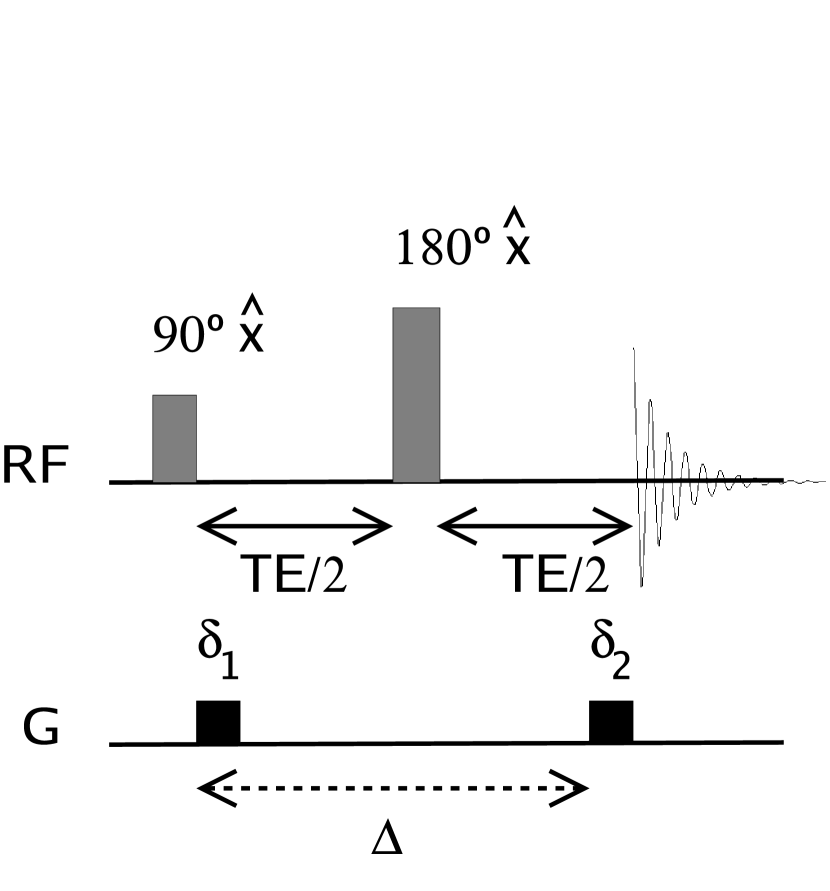
Figure 10.1: Stejskal-Tanner sequence. The large time interval $\Delta$ is the time from the start of the first gradient pulse to the start of the second gradient pulse. The RF pulse durations are assumed to be negligible in this analysis.

First we will look at a simple spin-echo sequence with two pulsed gradients shown in figure 10.1. This sequence was introduced by Stejskal and Tanner [53] and is often called Stejskal-Tanner (ST) sequence or a “pulsed-gradient spin-echo” sequence.

10.1.1 Initial Magnetization

We will start with fully relaxed longitudinal magnetization

$$M_{\parallel}^{0}=M_{0},$$ (10.1)

which implies zero transverse magnetization

$$M_{\perp}^{0}=0.$$ (10.2)

We have denoted the longitudinal and transverse magnetization with the superscript $0$ to designate the initial condition.

10.1.2 Excitation Pulse

The first RF pulse is a $90^{\circ}$ pulse. This excites all of the magnetization into the transverse plane. We use the superscript $90$ to denote the magnetization state after the $90^{\circ}$ pulse. The phase of the pulse is $\phi_{90}=0$ (denoted by $\hat{x}$ in the rotating frame) so we end up with our transverse magnetization along $\hat{y}$ (or the imaginary direction) after the pulse. We have, therefore,

$$M_{\parallel}^{90}=0,$$

$$M_{\perp}^{90}=i\,M_{0}.$$

The durations of both RF pulses in the sequence are assumed to be negligible compared to the gradient durations $\delta$ and the echo time $TE$.

10.1.3 Gradient Pulse $\delta$ without Relaxation or Diffusion

In general there will be $T_{1}$and $T_{2}^{*}$ relaxation occurring after excitation, but we will neglect this for the moment. Also, we will neglect diffusion for the moment and look at the solution to the Bloch equation in the presence of the gradient pulse. In the rotating frame the Bloch equation is

$$\frac{d\vec{M}}{dt}=\gamma\,\vec{M}\times[G_{s}(t)\,s\,\hat{z}],$$

which is equation 8.5 with only the gradient term. The gradient is along the arbitrary direction $\hat{s}$ and $s$ is the distance along $\hat{s}$ from the origin.

By neglecting relaxation, we need only consider the Bloch equation for the transverse component (in complex form)

$$\frac{\partial M_{\bot}}{\partial t}=-i\,\gamma\,M_{\bot}G_{s}(t)\,s.$$ (10.3)

We can divide both sides by $M_{\bot}$

$$\frac{\partial M_{\bot}}{M_{\bot}}=-i\,\gamma\,G_{s}(t)\,s\,\partial t,$$ (10.4)

and integrate to get

$$ln(\frac{M_{\bot}}{M_{\perp}^{initial}})=-i\,\gamma\,s\int_{0}^{t}G_{s}(t^{\prime})\,dt^{\prime}.$$ (10.5)

The solution to 10.4 becomes

$$M_{\bot}(s,\,t)=M_{\perp}^{initial}e^{-i\,2\,\pi\,q(t)\,s}.$$ (10.6)

Equation 10.6 is “staircase” twisted transverse magnetization as shown in figure 6.1. We have defined

$$q(t)\equiv\frac{\gamma}{2\,\pi}\int_{0}^{t}G_{s}(t^{\prime})\,dt^{\prime}.$$ (10.7)

This says that the instantaneous pitch of the magnetization twist along $\hat{s}$ is equal to the integral over time of the gradient.

10.1.4 Gradient Pulse $\delta$ with Diffusion

The effect of diffusion will be to introduce a time-dependent term to the solution in equation 10.6, which for now we can assume to be complex valued (it could alter the phase of the magnetization)

$$M_{\bot}(s,\,t)=A(t)\,M_{\perp initial}e^{-i\,2\,\pi\,q(t)\,s}.$$ (10.8)

We insert this into the transverse Bloch equation in the rotating frame (this time with the diffusion term)

$$\frac{\partial M_{\bot}}{\partial t}=-i\,\gamma\,M_{\bot}G_{s}(t)\,s+\nabla\cdot\mathbf{D}\nabla M_{\perp}.$$ (10.9)

Since the only spatial variation in $M_{\bot}$ is along $\hat{s}$ we can replace $\nabla\cdot\mathbf{D}\nabla M_{\perp}$ with $D_{s}\frac{\partial^{2}M_{\bot}}{\partial s^{2}}$ to get

$$\frac{\partial M_{\bot}}{\partial t}=-i\,\gamma\,M_{\bot}G_{s}(t)\,s+D_{s}\frac{\partial^{2}M_{\bot}}{\partial s^{2}}.$$ (10.10)

Substituting 10.8 into the spatial and temporal derivatives in 10.10 we have

$$\frac{\partial M_{\bot}}{\partial t}=-i\,2\,\pi\frac{\partial q(t)}{\partial t}A(t)\,M_{\perp initial}e^{-i\,2\,\pi\,q(t)\,s}+\frac{\partial A(t)}{\partial t}\,M_{\perp initial}e^{-i\,2\,\pi\,q(t)\,s}$$ (10.11)

and

$$D_{s}\frac{\partial^{2}M_{\bot}}{\partial s^{2}}=-4\,D_{s}\pi^{2}q^{2}(t)\,A(t)\,M_{\perp initial}e^{-i\,2\,\pi\,q(t)\,s}.$$ (10.12)

These lead to the following equation for $A(t)$

$$\frac{\partial A(t)}{\partial t}=-4\,D_{s}\pi^{2}q^{2}(t)\,A(t).$$ (10.13)

We can divide both sides by $A(t)$ and integrate to get

$$ln[\frac{A(t)}{A_{0}}]=-4\,D_{s}\pi^{2}\int_{0}^{t}q^{2}(t^{\prime})\,dt.$$ (10.14)

We can set $A_{0}=1$ and put this into the form

$$A(t)=e^{-b(t)\,D_{s}},$$ (10.15)

with the $b-value$ defined as

$$b(t)\equiv 4\,\pi^{2}\int_{0}^{t}q^{2}(t^{\prime})\,dt.$$ (10.16)

Our general solution for the transverse magnetization in the presence of diffusion and an applied gradient becomes

$$M_{\bot}(s,\,t)=M_{\perp initial}e^{-b(t)\,D_{s}}e^{-i\,2\,\pi\,q(t)\,s}.$$ (10.17)

After the gradient of duration $\delta$ in the superscript notation we have

$$M_{\parallel}^{\delta}=M_{\parallel}^{90}=0,$$ (10.18)

$$M_{\bot}^{\delta}=M_{\perp}^{90}e^{-b(\delta)\,D_{s}}e^{-i\,2\,\pi\,q(\delta)\,s}=i\,M_{0}e^{-b(\delta)\,D_{s}}e^{-i\,2\,\pi\,q(\delta)\,s}.$$ (10.19)

10.1.5 $\frac{TE}{2}$ Delay

The situation during the rest of $\frac{TE}{2}$ is much the same as during $\delta$ except there is no gradient so $q$ is constant. The $b-value$, however, will continue to evolve during this period. We have

$$M_{\parallel}^{\frac{TE}{2}}=0$$ (10.20)

and

$$M_{\bot}^{\frac{TE}{2}}=i\,M_{0}e^{-b(\frac{TE}{2})\,D_{s}}e^{-i\,2\,\pi\,q(\delta)\,s}$$ (10.21)

at the time $\frac{TE}{2}$ just before the $180^{\circ}$ pulse.

10.1.6 $180^{\circ}$ Pulse

The effect of the $180^{\circ}$ pulse is to invert the $\hat{y}$ component of the transverse magnetization. It would also invert the longitudinal magnetization if present. Note that the sign of the imaginary argument of the exponential (the gradient twist) is reversed. We can think of this as a change of the sign of $q$, giving

$$M_{\parallel}^{180}=0$$ (10.22)

and

$$M_{\bot}^{180}=-i\,M_{0}e^{-b(\frac{TE}{2})\,D_{s}}e^{i\,2\,\pi\,q(\frac{TE}{2})\,s}.$$ (10.23)

10.1.7 Second $\frac{TE}{2}$ Delay

At the end of the second $\frac{TE}{2}$ delay, the phase acquired during the first $\frac{TE}{2}$ delay due to inhomogeneity (or chemical shift) will cancel. This is due to the change in the sense of the helix due to any field (we have only included the Gradient explicitly) by the $180^{\circ}$ Pulse. Since attenuation due to diffusion depends on $q^{2}$, the attenuation continues to accumulate as during the first $\frac{TE}{2}$ delay. Just before the second gradient pulse $\delta 2$ we have

$$M_{\parallel}^{TE}=0$$ (10.24)

and

$$M_{\bot}^{TE-\delta}=-i\,M_{0}e^{-b(TE-\delta)\,D_{s}}e^{i\,2\,\pi\,q(\delta)\,s}.$$ (10.25)

10.1.8 Second Gradient Pulse $\delta_{2}$

First we will make a few observations. We will want $q(\Delta+\delta_{2})=0$ when we acquire the FID, otherwise the transverse magnetization is still twisted, and the signal is spoiled. This means that the area of the first gradient should be equal and opposite to the area of the second gradient or $\delta=\delta_{2}$. However, in figure 10.1 the two gradients have the same positive area. What we must remember is the effect of the $180^{\circ}$ pulse. The effect of the pulse is to reverse the imaginary ($\hat{y}$) component of $M_{\bot}$ which in our complex notation meant changing the sign of the $q$ accumulated before the pulse. Now the two positive gradients will cancel since they are on opposite sides of the $180^{\circ}$ pulse. We see this mathematically as

$$M_{\parallel}^{\delta_{2}}=0$$ (10.26)

and

$$M_{\bot}^{\delta_{2}}=-i\,M_{0}e^{-b(\Delta+\delta_{2})\,D_{s}}e^{i\,2\,\pi\,q(\delta)\,s}e^{-i\,2\,\pi\,q(\Delta+\delta_{2})\,s}=-i\,M_{0}e^{-b(\Delta+\delta_{2})\,D_{s}}.$$ (10.27)

10.1.9 Acquisition of FID

	$G_{s}(t)$	$q(t)$	$b(t)$
$t<0$	$0$	$0$	$0$
$0\leq t<\delta$	$G_{s}$	$\frac{\gamma}{2\pi}G_{s}t$	$\gamma^{2}G_{s}^{2}\frac{t^{3}}{3}$
$\delta\leq t<\frac{TE}{2}$	$0$	$\frac{\gamma}{2\pi}G_{s}\delta$	$\gamma^{2}G_{s}^{2}[\frac{\delta^{3}}{3}+\delta^{2}(t-\delta)]$
$\frac{TE}{2}\leq t<\Delta$	$0$	-$\frac{\gamma}{2\pi}G_{s}\delta$	$\gamma^{2}G_{s}^{2}[\frac{\delta^{3}}{3}+\delta^{2}(t-\delta)]$
$\Delta\leq t<\Delta+\delta_{2}$	$G_{s}$	-$\frac{\gamma}{2\pi}G_{s}[\delta-(t-\Delta)]$	$\gamma^{2}G_{s}^{2}[\frac{\delta^{3}}{3}-\delta^{3}+\delta^{2}\Delta+\frac{(t-\Delta-\delta)^{3}}{3}]$
$t\geq\Delta+\delta_{2}$	$0$	$0$	$\gamma^{2}G_{s}^{2}\delta^{2}(\Delta-\frac{\delta}{3})$

Table 10.1: $G_{s}(t)$, $q(t)$ and $b(t)$. $\delta_{1}=\delta_{2}=\delta$

Now we evaluate $q(t)$ and $b(t)$ given $G_{s}(t)$ at different time points along the sequence. Table 10.1 shows the results. The $b-value$ at the spin echo time $TE=\Delta+\delta_{2}$ is then

$$b(TE)=\gamma^{2}G_{s}^{2}\delta^{2}(\Delta-\frac{\delta}{3}),$$ (10.28)

the well known result for a ST sequence. The $b-value$ determines the sensitivity of the sequence to diffusion. If the $b-value$ is small or zero then the sequence is not sensitive to diffusion. If the sequence has a significant $b-value$ it is called “diffusion weighted.”

10.1.10 $T_{2}$ Relaxation

We will show in the next section 10.2 equation 10.46 that $T_{2}$ relaxation and diffusion effects are separable so that we can write the final FID signal for our ST spin-echo as

$$M_{\bot}^{\delta 2}=-i\,M_{0}e^{-b(TE)\,D_{s}}e^{-\frac{TE}{T_{2}}}.$$ (10.29)

10.2 Stimulated Echo

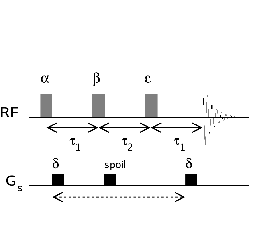
Figure 10.2: Stimulated-Echo sequence. Again, the large time interval $\Delta$ includes one of the small gradient pulse duration intervals $\delta$.

The stimulated echo was first reported by E. L. Hahn [41, fig. 6g]. The sequence (see figure 10.2) is similar to a spin echo sequence. The major difference is that the $180^{\circ}$ pulse is split into two pulses with a delay in between. The path that the magnetization leading to the final FID takes is longitudinal between the last two pulses. Also there is a 50% loss of signal in all but the ideal perfectly homogeneous no-gradient case, due to the process of rotating the twisted transverse magnetization helix into the longitudinal direction. The major advantage of the stimulated echo sequence is that during the $\tau_{2}$ time period there is no $T_{2}$ relaxation[61, 62]. This potentially allows a long $\Delta$ without losing as much signal as in a spin echo if $T_{2}<T_{1}$.

We can analyze the stimulated echo in a similar manner to the spin echo, using some of our previous results for the attenuation of transverse magnetization due to diffusion. In addition we will see that we need a similar expression for the attenuation due to diffusion of longitudinal magnetization.

10.2.1 Initial Magnetization

We will introduce relaxation and arbitrary RF pulse angles and phases into the analysis. Before the $\alpha$ pulse we have

$$M_{\|}^{0}=M_{0}$$ (10.30)

and

$$M_{\bot}^{0}=0.$$ (10.31)

10.2.2 $\alpha$ Pulse

After the $\alpha$ pulse we have

$$M_{\|}^{\alpha}=cos(\alpha)\,M_{\|}^{0}-sin(\alpha)\,Im(e^{-i\,\phi_{\alpha}}M_{\bot}^{0})=cos(\alpha)\,M_{0}$$ (10.32)

and

$$M_{\bot}^{\alpha}=[Re(e^{i\,\phi_{\alpha}}M_{\bot}^{0})+i\,cos(\alpha)\,Im(e^{i\,\phi_{\alpha}}M_{\bot}^{0})]\,e^{-i\,\phi_{\alpha}}+i\,sin(\alpha)\,e^{i\,\phi_{\alpha}}M_{\|}^{0}=+i\,sin(\alpha)\,e^{i\,\phi_{\alpha}}M_{0}.$$ (10.33)

This assumes that during the RF pulse all other terms (relaxation, diffusion) in the Bloch equations are negligible and that the pulse is on-resonance. $\phi_{\alpha}$ is the phase of the RF pulse, corresponding to the orientation of the $B_{1}$ field in the rotating frame. $\alpha$ is the flip angle. $Re$ and $Im$ correspond to the real and imaginary parts of their argument. The above are solutions to the Bloch equations for the condition

$$\frac{\partial\alpha}{\partial t}=\gamma B_{1},$$ (10.34)

leading to the equation for $\alpha$

$$\alpha=\gamma\int_{0}^{t}B_{1}dt.$$ (10.35)

10.2.3 1st Gradient $\delta$

The effect of the gradient is to twist the transverse magnetization along the direction $\hat{s}$. $q$ is $q(\delta)$ as defined in equation 10.7. We already know that we need to consider diffusion during the period $\delta$ from section 10.1. We will also consider relaxation, but neglect off-resonance and inhomogeneity effects. We will assume a solution of the form

$$M_{\perp}=e^{-i\,2\pi\,q\,s}A_{\perp}(\tau_{1})\,R_{\perp}(\tau_{1})\,M_{\perp}^{\alpha},$$ (10.36)

and substitute into the rotating frame Bloch equation

$$\frac{dM_{\perp}}{dt}=\gamma\,[\vec{M}_{\perp}\times\vec{G}_{s}s]_{\perp}-\frac{M_{\perp}}{T_{2}}+\nabla\cdot\mathbf{D}\nabla M_{\perp},$$ (10.37)

where $A$ is the attenuation due to diffusion and $R$ due to relaxation. We can expand out the cross product (using equation 8.6) and since the spatial variation of $M_{\perp}$ is only along $\hat{s}$ we get

$$\frac{dM_{\perp}}{dt}=-i\,\gamma\,M_{\perp}G_{s}s-\frac{M_{\perp}}{T_{2}}+D_{s}\frac{\partial^{2}M_{\perp}}{\partial s^{2}}.$$ (10.38)

Substituting 10.36 into 10.38 we get constraint equations for $q$, $A_{\perp}$and $R_{\perp}$

$$\frac{\partial q}{\partial t}=\frac{\gamma}{2\pi}G_{s},$$ (10.39)

$$\frac{\partial R_{\perp}}{\partial t}=-\frac{R_{\perp}}{T_{2}},$$ (10.40)

and

$$\frac{\partial A_{\perp}}{\partial t}=-4\,\pi^{2}q^{2}A_{\perp},$$ (10.41)

These have the corresponding solutions (with the additional constraint that all go to $1$ at $t=0$)

$$q=\frac{\gamma}{2\pi}\int_{0}^{t}G_{s}dt^{\prime},$$ (10.42)

$$R_{\perp}=e^{-\frac{t}{T_{2}}},$$ (10.43)

and

$$A_{\perp}=e^{-b(t)\,D_{s}}$$ (10.44)

with

$$b(t)\equiv 4\,\pi^{2}\int_{0}^{t}q^{2}dt^{\prime}.$$ (10.45)

All of this is consistent with the results in section 10.1 except that we have allowed the excitation pulse to have arbitrary rotation angle and phase and added $T_{2}$ relaxation. The solution is

$$M_{\bot}^{\delta}=e^{-i\,2\pi\,q\,s}A_{\perp}(\delta)\,R_{\perp}(\delta)\,M_{\bot}^{\alpha}=i\,sin(\alpha)\,e^{i\,\phi_{\alpha}}e^{-i\,2\pi\,q\,s}e^{-b(\delta)\,D_{s}}e^{-\frac{\delta}{T_{2}}}M_{0}.$$ (10.46)

The longitudinal magnetization is not affected by the gradient, and will only experience $T_{1}$ relaxation. The result is

$$M_{\|}^{\delta}=M_{0}-(M_{0}-M_{\|}^{\alpha})\,e^{-\frac{\delta}{T_{1}}}=M_{0}-[M_{0}-cos(\alpha)\,M_{0}]\,e^{-\frac{\delta}{T_{1}}},$$ (10.47)

which is a solution to the equation

$$\frac{dM_{\parallel}}{dt}=\frac{(M_{0}-M_{\parallel})}{T_{1}}.$$ (10.48)

The longitudinal magnetization has no spatial variation so there will be no diffusional effects at this point ($\nabla\cdot\mathbf{D}\nabla M_{\parallel}=0$).

10.2.4 $\tau_{1}$ Delay

We now consider the delay $\tau_{1}$, which we will make inclusive of the delay $\delta$. We will again neglect off-resonance effects, and since there are no gradient or RF pulses we will be left with relaxation and diffusion. This is the same situation as during the $\delta$ delay, except that $q$ is constant after $\delta$. We can re-use the results from above to get

$$M_{\bot}^{\tau_{1}}=e^{-i\,2\pi\,q\,s}A_{\perp}(\tau_{1})\,R_{\perp}(\tau_{1})\,M_{\bot}^{\alpha}=i\,sin(\alpha)\,e^{i\,\phi_{\alpha}}e^{-i\,2\pi\,q\,s}e^{-b(\tau_{1})\,D_{s}}e^{-\frac{\tau_{1}}{T_{2}}}M_{0}$$ (10.49)

and

$$M_{\|}^{\tau_{1}}=M_{0}-(M_{0}-M_{\|}^{\alpha})\,e^{-\frac{\tau_{1}}{T_{1}}}=M_{0}-[M_{0}-cos(\alpha)\,M_{0}]\,e^{-\frac{\tau_{1}}{T_{1}}}.$$ (10.50)

10.2.5 $\beta$ Pulse

We handle the $\beta$ RF pulse similarly to $\alpha$, assuming that the pulse is short enough so that there is no relaxation or diffusional attenuation. The difference is that now we have non-zero transverse magnetization which will be rotated into the longitudinal direction. We will see that this longitudinal magnetization has spatially varying amplitude (and will be subject to diffusional attenuation during subsequent delays).

We will assume that the transverse magnetization after the $\beta$ pulse is immediately spoiled by the gradient, we now have

$$M_{\|}^{\beta}=cos(\beta)\,M_{\|}^{\tau_{1}}-sin(\beta)\,Im(e^{-i\,\phi_{\beta}}M_{\bot}^{\tau_{1}})$$

$$=cos(\beta)\,\{M_{0}-[M_{0}-cos(\alpha)\,M_{0}]\,e^{-\frac{\tau_{1}}{T_{1}}}\}-sin(\beta)\,Im(e^{-i\,\phi_{\beta}}i\,sin(\alpha)\,e^{i\,\phi_{\alpha}}e^{-i\,2\pi\,q\,s}e^{-b(\tau_{1})\,D_{s}}e^{-\frac{\tau_{1}}{T_{2}}}M_{0})$$ (10.51)

and

$$M_{\bot}^{\beta}=0.$$ (10.52)

10.2.6 $\tau_{2}$ Delay

During the $\tau_{2}$ delay the longitudinal component obeys the Bloch equation

$$\frac{dM_{\parallel}}{dt}=\frac{(M_{0}-M_{\parallel})}{T_{1}}+D_{s}\frac{\partial^{2}M_{\parallel}}{\partial s^{2}},$$ (10.53)

where we have made the substitution $\nabla\cdot\mathbf{D}\nabla M_{\parallel}=D_{s}\frac{\partial^{2}M_{\parallel}}{\partial s^{2}}$ since all spatial variation of $M_{\parallel}$ is along $\hat{s}$. We can further break $M_{\parallel}$ into a spatially constant $M_{\parallel cnst}$ part and a spatially varying $M_{\parallel}(s)$ part. After substituting $M_{\parallel}=M_{\parallel cnst}+M_{\parallel}(s)$ into equation 10.53 we have

$$\frac{dM_{\parallel cnst}}{dt}=\frac{(M_{0}-M_{\parallel cnst})}{T_{1}}$$ (10.54)

and

$$\frac{dM_{\parallel}(s)}{dt}=-\frac{M_{\parallel}(s)}{T_{1}}+D_{s}\frac{\partial^{2}M_{\parallel}(s)}{\partial s^{2}}.$$ (10.55)

We already know the solution to equation 10.54: it is just $T_{1}$ relaxation. As it turns out we also know the solution to 10.55. It has exactly the same form as equation 10.38 but with no gradient (which means no change in $q$) and with $T_{2}$ replaced by $T_{1}$. The solutions are then

$$M_{\parallel cnst}=M_{0}-(M_{0}-M_{\parallel cnst,initial})e^{-\frac{\tau_{2}}{T_{1}}}$$ (10.56)

and

$$M_{\parallel}(s)=e^{-b_{\parallel}(\tau_{2})\,D_{s}}e^{-\frac{\tau_{2}}{T_{1}}}M_{\parallel initial}(s),$$ (10.57)

where $b_{\parallel}(t)$ has the same form as equation 10.45 but refers to the spatial variation $q$ of the longitudinal magnetization and the time interval $\tau_{2}$ only. Making the substitutions

$$M_{\parallel cnst,initial}=cos(\beta)\,\{M_{0}-[M_{0}-cos(\alpha)\,M_{0}]\,e^{-\frac{\tau_{1}}{T_{1}}}\}$$ (10.58)

and

$$M_{\parallel initial}(s)=-sin(\alpha)\,sin(\beta)\,cos[\phi_{\alpha}-\phi_{\beta}-2\pi q(\delta)\,s]\,e^{-b(\tau_{1})\,D_{s}}e^{-\frac{\tau_{1}}{T_{2}}}M_{0}$$ (10.59)

we get the rather complicated expression

$$M_{\parallel}^{\tau_{2}}=M_{0}-\{M_{0}-cos(\beta)\,\{M_{0}-[M_{0}-cos(\alpha)\,M_{0}]\,e^{-\frac{\tau_{1}}{T_{1}}}\}\}e^{-\frac{\tau_{2}}{T_{1}}}\\ -sin(\alpha)\,sin(\beta)\,cos[\phi_{\alpha}-\phi_{\beta}-2\pi q(\delta)\,s]\,e^{-[b(\tau_{1})+b_{\parallel}(\tau_{2})]\,D_{s}}e^{-\frac{\tau_{1}}{T_{2}}-\frac{\tau_{2}}{T_{1}}}M_{0}$$ (10.60)

and the relatively simple

$$M_{\perp}^{\tau_{2}}=0.$$ (10.61)

10.2.7 $\epsilon$ Pulse

The $\epsilon$ pulse is the final RF pulse. Before the $\epsilon$ pulse we have no transverse magnetization. Our observable signal must then come from magnetization that was longitudinal at the end of the $\tau_{2}$ delay. The effect of the $\epsilon$ pulse is to give

$$M_{\|}^{\epsilon}=cos(\epsilon)\,M_{\|}^{\tau_{2}}$$ (10.62)

and

$$M_{\bot}^{\epsilon}=i\,sin(\epsilon)\,e^{i\,\phi_{\epsilon}}M_{\|}^{\tau_{2}}.$$ (10.63)

After substitution of $M_{\|}^{\tau_{2}}$ we have

$$M_{\perp}^{\epsilon}=i\,sin(\epsilon)\,e^{i\,\phi_{\epsilon}}\{M_{0}-\{M_{0}-cos(\beta)\,\{M_{0}-[M_{0}-cos(\alpha)\,M_{0}]\,e^{-\frac{\tau_{1}}{T_{1}}}\}\}\,e^{-\frac{\tau_{2}}{T_{1}}}\\ -sin(\alpha)\,sin(\beta)\,cos[\phi_{\alpha}-\phi_{\beta}-2\pi q(\delta)\,s]\,e^{-[b(\tau_{1})+b_{\parallel}(\tau_{2})]\,D_{s}}e^{-\frac{\tau_{1}}{T_{2}}-\frac{\tau_{2}}{T_{1}}}M_{0}\}.$$ (10.64)

We can ignore the longitudinal component at this point as it will not contribute to the final signal. We would need to consider it if we were interested in the steady state magnetization for partial recovery.

10.2.8 Final Gradient and Delay

We now have enough information to know how the transverse component will behave without further derivation. We note that the final delay period is the same as the first period, $\tau_{1}$. Any phase acquired due to inhomogeneity during the first delay will be re-phased during the second delay. There is no phase acquired during the center delay, since the magnetization leading to the final observable signal interest was longitudinal.

During the final delay, which we take to include the last gradient $\delta$ at the end, we have

$$M_{\perp{}}^{\tau_{1}last}=e^{-i\,2\pi\,q(\delta)\,s}e^{-b(\tau_{1}last)\,D_{s}}e^{-\frac{\tau_{1}}{T_{2}}}M_{\perp}^{\epsilon}.$$ (10.65)

Substituting $cos(a)=\frac{e^{i\,a}+e^{-i\,a}}{2}$ for the $cos[\phi_{\alpha}-\phi_{\beta}-2\pi q(\delta)\,s]$ term in $M_{\perp}^{\epsilon}$ we get

$$M_{\perp}^{\tau_{1}last}=\\ i\,c_{\epsilon}\{M_{0}-\{M_{0}-cos(\beta)\,\{M_{0}-[M_{0}-cos(\alpha)\,M_{0}]\,e^{-\frac{\tau_{1}}{T_{1}}}\}\}\}e^{-\frac{\tau_{2}}{T_{1}}}e^{-i\,2\pi\,q(\delta)\,s}e^{-b(\tau_{1}last)\,D_{s}}e^{-\frac{\tau_{1}}{T_{2}}}\\ -i\,c_{\epsilon}sin(\alpha)\,sin(\beta)\,\frac{e^{i\,[\phi_{\alpha}-\phi_{\beta}-2\pi q(\delta)\,s]}}{2}\,e^{-[b(\tau_{1})+b_{\parallel}(\tau_{2})]\,D_{s}}e^{-\frac{\tau_{1}}{T_{2}}-\frac{\tau_{2}}{T_{1}}}M_{0}\,e^{-i\,2\pi\,q(\delta)\,s}e^{-b(\tau_{1}last)\,D_{s}}e^{-\frac{\tau_{1}}{T_{2}}}\\ -i\,c_{\epsilon}sin(\alpha)\,sin(\beta)\,\frac{e^{-i\,[\phi_{\alpha}-\phi_{\beta}-2\pi q(\delta)\,s]}}{2}\,e^{-[b(\tau_{1})+b_{\parallel}(\tau_{2})]\,D_{s}}e^{-\frac{\tau_{1}}{T_{2}}-\frac{\tau_{2}}{T_{1}}}M_{0}\,e^{-i\,2\pi\,q(\delta)\,s}e^{-b(\tau_{1}last)\,D_{s}}e^{-\frac{\tau_{1}}{T_{2}}},$$ (10.66)

where

$$c_{\epsilon}\equiv sin(\epsilon)\,e^{i\,\phi_{\epsilon}}.$$ (10.67)

We notice that only in the last term do the gradient twists cancel. We now assume that $q$ is large enough so that any signal that is twisted is spoiled and we end up with

$$M_{\perp}^{ste}=-\frac{i}{2}\,sin(\alpha)\,sin(\beta)\,sin(\epsilon)\,e^{-i\,(\phi_{\alpha}-\phi_{\beta}-\phi_{\epsilon})}e^{-b\,D_{s}}e^{-2\frac{\tau_{1}}{T_{2}}-\frac{\tau_{2}}{T_{1}}}M_{0},$$

where we have combined all the $b-values$ into

$$b=\gamma^{2}G^{2}\delta^{2}(\Delta-\frac{\delta}{3}).$$

The accumulated $b-value$ is identical to the ST sequence since during the $\tau_{2}$ period the longitudinal magnetization undergoes the same attenuation due to diffusion.

The pre-factor of $\frac{1}{2}$, corresponding to a %50 loss of signal not attributable to relaxation or diffusion, is due to the gradient not being able to simultaneously re-phase the counter-twisted components embodied in the 2nd term of equation 10.66.

Part II Distant Dipolar Field Effects

Chapter 11 DISTANT DIPOLAR FIELD

11.1 Introduction

In Part I we introduced the various physical effects considered relevant in liquid-state NMR, culminating in the Bloch equations (see chapter 8) for describing the classical macroscopic behavior of an ensemble of spins. Up to this point we have neglected the explicit contribution of the field from nuclear magnetization originating in the sample on other parts of the sample. This gives rise to two new effects.

One is called radiation damping, and is not directly felt by the sample, but requires a receiver coil to “feed back” an RF field into the sample. For the most part we will discuss radiation dampening as a nuisance to be avoided (Chapter 13).

Another is the distant dipolar field or DDF. The term DDF has actually been modified from “dipolar demagnetization field” [63, p. 49-61] and both are used in the literature, the former being an innovation of NMR researchers investigating dipolar field-induced echoes in liquids, or biological samples. It had been thought in liquids that static dipolar field effects, which are the source of many useful and confounding effects in spectroscopy and imaging of solids [64], could largely be neglected due to the averaging effects of diffusion.

The first sign that this was not true came from low-temperature physics experiments using solid ${}^{3}He$ in the late 1970’s and early ’80’s. Deville et al. observed unexpected “multiple spin echoes” in low temperature solid ${}^{3}He$, [65, 66, 67]. One reason for this is that even at low field the magnetization is very large due to the extremely low $\mu K$ temperatures.

Observation of multiple spin echoes in water at room temperature came in the early 1990s when Bowtell, Korber, and Warren, [68, 69, 70, 71] all reported echoes or effects they attributed to sample nuclear magnetization, coupled by the dipolar field. At first these claims were sometimes disputed and attributed to other sources, especially in the case of the Warren and collaborators 2d spectroscopy experiments [72, 70].

There has also been a lively discussion of the necessity to treat the DDF classically or quantum mechanically [73] as intermolecular multiple quantum coherence (iMQC). In general it has been shown that the classical description is adequate under most conditions, and in fact has lead to the quantification of many effects, such as diffusion weighting [74, 75], that have so far been intractable in the quantum picture.

Interest has grown steadily over the intervening years due to novel application possibilities. One of the first was the realization that signal weighting (contrast) was sensitive to so-called “meso-scale” structure [76, 77, 78]. Meso-scale is the term used to distinguish the scale intermediate between micro-scale processes, such as diffusion, $T_{1}$, and $T_{2}$, and macro-scale, such as a resolvable imaging voxel. In other words, DDF based sequences could probe sub-voxel structure with scale larger than the diffusion distance. This novel imaging contrast mechanism has continued to be pursued [79, 80, 81, 82, 83, 84].

The Holy Grail of in-vivo magnetic resonance spectroscopy (MRS) is the ability to localize and quantify metabolite peaks at high resolution and high signal-to-noise ratio. Several DDF sequences offer the possibility of obtaining higher resolution spectra than obtainable with conventional NMR sequences. The first implemented was HOMOGENIZED [2, 85] which stands for “homogeneity enhancement by intermolecular zero-quantum detection.” Its usefulness has been demonstrated already for non-localized spectroscopy of live animals and excised tissue [86]. HOMOGENIZED continues to be an active research area with improved understanding of relaxation and diffusion effects and water suppression being recently reported [87, 75, 88, 89]. Other variations of HOMOGENIZED have been proposed as well [90, 88].

11.2 Field of a Dipole

The field due to a single magnetic dipole is

$$\vec{B}_{dip}=\frac{\mu_{0}}{4\pi}\frac{3\,(\vec{\mu}\cdot\hat{r})\,\hat{r}-\vec{\mu}}{r^{3}}.$$ (11.1)

and is plotted in figure 11.1.

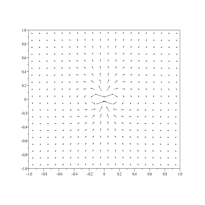
Figure 11.1: Field due to single point dipole $\vec{\mu}=\mu\,\hat{z}$. The $\hat{x}$ axis is along the horizontal, $\hat{z}$ along the vertical. The field is symmetric about the $\hat{z}$ axis. The plotted $r$ dependence has been changed from $\frac{1}{r^{3}}$ to $\frac{1}{r}$ in order to aid visualization.

In most circumstances of interest, the secular component (see A.4) of $\vec{B}_{dip}$ is the only component that will contribute in the presence of a much stronger externally applied field $\vec{B}_{0}=B_{0}\hat{z}$. The secular component of the field is

$$\vec{B}_{secular}=\frac{\mu_{0}}{4\pi}\frac{1}{r^{3}}[\frac{3\,cos^{2}(\theta)-1}{2}]\,(3\,\mu_{z}\hat{z}-\vec{\mu}).$$ (11.2)

The range of validity of the approximation (that the non-secular components are negligible) can be estimated from the condition,

$$B_{0}\gg\frac{\mu_{0}}{4\pi}\frac{1}{r^{3}}|\vec{\mu}|.$$ (11.3)

In a liquid, diffusion will determine the minimum $r$ that need be considered. In a solid it is lattice parameters and exchange. The angular dependence of the secular field deserves some attention. First of all we notice that it is the Legendre polynomial

$$P_{2}[cos(\theta)]=\frac{3\,cos^{2}(\theta)-1}{2}.$$ (11.4)

In the DDF/iMQC literature the angular dependence is often defined as

$$\Lambda(\vec{r})\equiv\frac{3\,(\hat{r}\cdot\hat{z})^{2}-1}{2}=\frac{3\,cos^{2}(\theta)-1}{2}.$$ (11.5)

The zeros of $\Lambda$ are at the so called “magic angle”

$$cos(\theta_{magic})=_{-}^{+}\sqrt{\frac{1}{3}}$$ (11.6)

or

$$\theta_{magic}=_{-}^{+}54.73561^{\circ}.$$ (11.7)

At this angle the secular field of a dipole disappears, regardless of the orientation or magnitude of $\vec{\mu}$. We plot $\Lambda$ in figure 11.2.

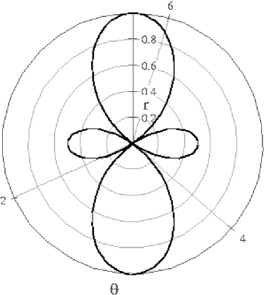
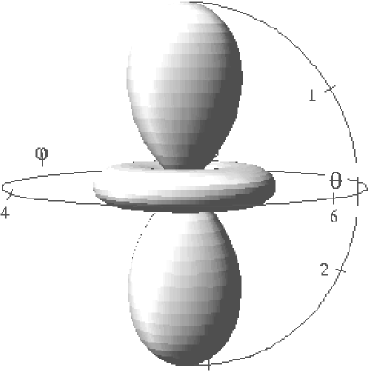
Figure 11.2: Angular dependence, $\Lambda(\vec{r})$, of the secular field of a dipole. Note that the polarity of $\Lambda$ is positive in the upper and lower lobes and negative in the side lobes (toroidal lobe in 3d).

11.3 Secular Dipolar Demagnetizing Field

The secular dipolar demagnetizing field from a distribution of magnetization takes the form [65, 91, 92]

$$\vec{B}_{d}(\vec{r})=-\frac{\mu_{0}}{4\pi}\int_{\infty}d^{3}r^{\prime}\,\frac{\Lambda(\vec{r}-\vec{r}^{\prime})}{|\vec{r}-\vec{r}^{\prime}|^{3}}\,[3\,M_{z}(\vec{r}^{\prime})\,\hat{z}-\vec{M}(\vec{r}^{\prime})],$$ (11.8)

with

$$\Lambda(\vec{r})\equiv\frac{3\,(\hat{r}\cdot\hat{z})^{2}-1}{2}.$$ (11.9)

This is the field that a spin or small ensemble of spins “feels” due to all other spins (magnetization) in the sample.

11.8 is in fact the convolution

$$\vec{B}_{d}(\vec{r})=-\frac{\mu_{0}}{4\pi}\frac{\Lambda(\vec{r})}{r^{3}}*[3\,M_{z}(\vec{r})\,\hat{z}-\vec{M}(\vec{r})].$$ (11.10)

We then take the three-dimensional Fourier transform of $\vec{B}_{d}(\vec{r})$

$$\mathcal{F}_{3}\{\vec{B}_{d}(\vec{r})\}\equiv\vec{B}_{d}(\vec{\rho})=\int_{\infty}d^{3}r\,e^{-i\,2\pi\,\vec{\rho}\cdot\vec{r}}\vec{B}_{d}(\vec{r}),$$ (11.11)

which by the convolution theorem [93, section 3.3.6, p. 124-28] is

$$\vec{B}_{d}(\vec{\rho})=-\frac{\mu_{0}}{4\pi}\mathcal{F}_{3}\{\frac{\Lambda(\vec{r})}{r^{3}}\}\,\mathcal{F}_{3}\{3\,M_{z}(\vec{r})\,\hat{z}-\vec{M}(\vec{r})\}.$$ (11.12)

For now we will not worry about the explicit form of $\vec{M}(\vec{r})$ and use the general form

$$\mathcal{F}_{3}\{3\,M_{z}(\vec{r})\,\hat{z}-\vec{M}(\vec{r})]\}=3\,M_{z}(\vec{\rho})\,\hat{z}-\vec{M}(\vec{\rho}).$$ (11.13)

The transform of the convolution kernel $\frac{\Lambda(\vec{r})}{r^{3}}$ from reference [65] and Appendix A.3 is

$$\mathcal{F}_{3}\{\frac{\Lambda(\vec{r})}{r^{3}}\}=-\frac{4\pi}{3}\Lambda(\vec{\rho}).$$ (11.14)

and the result for the transform of

$$\vec{B}_{d}(\vec{\rho})=\frac{1}{3}\Lambda(\vec{\rho})\,[3\,M_{z}(\vec{\rho})\,\hat{z}-\vec{M}(\vec{\rho})].$$

11.4 “local” form

Deville et al. [65, section B] noted that if the sample magnetization is periodic the contribution of the sample magnetization to the dipolar field becomes localized.

One can visualize this as follows (see figure 11.3). When one looks far from the point of interest where one is computing the field, there are regions of positive and negative magnetization, at approximately the same distance and angle. This leads to an “effective magnetization” which is the spatial average. The effective magnetization is zero, leading to a contribution to the dipolar field of zero. Close to the point of interest the differing regions of magnetization have significantly different distance or angle, and do not cancel. This is a “Sphere of Lorentz” argument, similar to the line of reasoning presented in [94, 12]. This line of reasoning applies to the dipolar field from both longitudinal and transverse magnetization. In the transverse case, the magnetization is complex-valued and we can visualize the real and imaginary component separately.

Mathematically we can state the localization as follows. Consider two regions of the sample, separated by half the modulation period. The two location vectors are $\vec{r}_{1}$and $\vec{r}_{2}$. First, assuming they have the same equilibrium magnetization and relaxation properties, we can write their contribution to the dipolar field (at $r$=0 for convenience) as

$$\vec{b}_{d,\,1}=\frac{\mu_{0}}{4\pi}\delta v\frac{\Lambda(\vec{r}_{1})}{r_{1}^{3}}\,\vec{M}^{\prime}(\vec{r}_{1}),$$ (11.15)

$$\vec{b}_{d,\,2}=\frac{\mu_{0}}{4\pi}\delta v\frac{\Lambda(\vec{r}_{2})}{r_{2}^{3}}\,\vec{M^{\prime}}(\vec{r}_{2}),$$ (11.16)

with

$$\vec{M^{\prime}}(\vec{r})\equiv 3\,M_{z}(\vec{r})\,\hat{z}-\vec{M}(\vec{r})$$ (11.17)

and

$$\vec{r}_{2}=\vec{r}_{1}+\frac{\vec{\delta r}}{2}$$ (11.18)

where $\vec{\delta r}$ is the period of the modulation. If the magnetization is smoothly varying compared to the scale of modulation we have

$$\vec{M}(\vec{r}_{1})\approx-\vec{M}(\vec{r}_{2}).$$ (11.19)

The volume of the region under consideration, $\delta v$, is such that $\delta v\leq(\frac{\delta r}{2})^{3}$.

We write

$$\vec{\delta b}=\frac{\vec{b}_{d,\,2}+\vec{b}_{d,\,1}}{2}$$ (11.20)

keeping in mind that we can consider all such pairs of magnetized regions in the sample once (i.e. don’t double count).

Substituting into 11.20 and keeping all first-order terms in $\vec{\delta r}$ gives us

$$\vec{\delta b}\approx\frac{\mu_{0}}{4\pi}\delta v\,\{\frac{1}{r_{1}^{3}}[1-\frac{3}{2}(\hat{r}_{1}\cdot\hat{\delta r})\,\frac{\delta r}{r_{1}}]-\frac{1}{r_{1}^{3}}\}\,\Lambda(\vec{r}_{1})\,\vec{M}^{\prime}(\vec{r}_{1}),$$

which after simplification gives

$$\vec{\delta b}\approx\frac{\mu_{0}}{4\pi}\delta v\,\frac{1}{r_{1}^{3}}[-\frac{3}{2}(\hat{r}_{1}\cdot\hat{\delta r})\,\frac{\delta r}{r_{1}}]\,\Lambda(\vec{r}_{1})\,\vec{M}^{\prime}(\vec{r}_{1}).$$

When considering integration over the entire sample we see that modulation has introduced a weighting factor of

$$W=-\frac{3}{2}(\hat{r}\cdot\hat{\delta r})\,\frac{\delta r}{r}$$

when we consider magnetized regions of the sample in the pairwise manner above.

At this point we can say that the dipolar field originates primarily from magnetization within a radius of $r\sim\delta r$ . Magnetization from outside that radius contributes less significantly. The weighting further favors magnetization along the direction of the modulation, and penalizes magnetization orthogonal to the modulation (see right figure 11.3).

Although not arrived at by this argument, $\delta r$ is also the so-called “correlation distance” used in the DDF literature. The correlation distance is the distance over which the DDF $\vec{B}_{d}$ is assumed to act in a structured sample. Contributions from farther than $\delta r$ are assumed to be negligible.

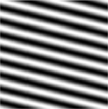
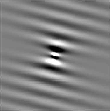
Figure 11.3: Modulated Magnetization. Weighted Contribution to DDF.

Magnetization is shown on the left. The weighted contribution of the magnetization to the dipolar field at the center is shown on the right. Far from the center there is a weight of zero. While the figure is shown in 2d, the localization applies in 3d as well, the weighting being symmetric about the gradient axis through the center. The $\vec{B}_{d}$ experienced at the center of the plotted region will be the integral over the 3d volume.

11.5 When does this break down?

There are several conditions under which the localization effect of modulating the magnetization will break down. The underlying cause of the breakdown is that nearby regions of magnetization far from the point of interest for the $B_{d}$ calculation no longer cancel.

At the edges of a sample of finite extent (in other words, all real samples) there will be a volume whose paired volume needed for cancellation lies outside the sample boundary, which is assumed to have zero magnetization. This can result in magnetization far from the point of interest contributing to $B_{d}$. One good assumption is that if the sample boundary is far enough away (so that $r\gg\delta r$) from the point of interest the contribution of this magnetization will be small.

Another case is when the underlying structure of the sample has variation near the scale of the modulation. This is a violation of the “slowly varying” condition for $\vec{M}(\vec{r})$. This results in a failure of the cancellation condition, potentially over large volumes of the sample and not necessarily far from the point of interest. This effect had been predicted [91], and more recently observed [95, 96] and dubbed “NMR Diffraction.”

It is ironic that this sensitivity to underlying magnetization modulation or structure relative to the applied modulation has also been proposed as a contrast method for DDF weighted MRI [97], or for potential quantization of bone density [98]. The irony comes from the fact that there is a desire to localize a contrast that has an inherent non-locality associated with it. There has been some reporting of the difficulties due to this [99], but it is still an active topic of investigation.

11.6 “point” form

We can gain further insight for calculation of $\vec{B}_{d}(\vec{r})$. This was again first suggested by Deville et al. [65, eq. (9)]. The idea is that when $\vec{M}(\vec{r})$ is constant (or stretched to the less stringent condition of changing slowly or is “slowly varying” compared to $\hat{\delta r}$) we can approximate the dipolar field $\vec{B}_{d}(\vec{r})$ as proportional to $\vec{M}^{\prime}(\vec{r})$. In other words, the spatial integration of equation 11.8 (or convolution of 11.10) disappears, and we have (using equation 11.17) the proportional relationship

$$\vec{B}_{d}(\vec{r})\propto\Lambda(\vec{r})\,\vec{M}^{\prime}(\vec{r}).$$ (11.21)

Deville et al. justify this as follows (in our notation).

First we note that the Fourier transform of $\vec{B}_{d}(\vec{r})$ has the form

$$\mathcal{F}_{3}\{\vec{B}_{d}(\vec{r})\}\equiv\vec{B}_{d}(\vec{\rho})=\frac{\mu_{0}}{3}\Lambda(\vec{\rho})\,[3\,M_{z}(\vec{\rho})\,\hat{z}-\vec{M}(\vec{\rho})],$$ (11.22)

and note that the convolution operation leads to a product in the transform space. We can write as

$$\vec{B}_{d}(\vec{\rho})=\mathbf{C_{\hat{\rho}}}\vec{M}(\vec{\rho}),$$ (11.23)

where $\mathbf{C}_{\hat{\rho}}$ is a 3x3 matrix or tensor that depends only on the direction $\hat{\rho}$, not on the radius.

When the dominant variation in $\vec{M}(\vec{r})$ is one-dimensional, with constant (or slowly varying) value orthogonal to direction $\hat{s}$, we can define

$$\vec{M}(\vec{r})\approx\vec{M}(\hat{s}\cdot\vec{r})\equiv\vec{M}(s).$$ (11.24)

We perform the 3d Fourier transform of $\vec{M}(s)$,

$$\mathcal{F}_{3}\{\vec{M}(s)\}=\vec{M}(\rho_{s})\,\delta_{2}(\rho_{s}),$$ (11.25)

where $\delta_{2}(\rho_{s})$ represents a plane delta function orthogonal to the direction $\hat{s}$, and $\rho_{s}\equiv\vec{\rho}\cdot\hat{s}$. The $\rho_{s}$ dependence is not altered by $\mathbf{C}$. We now have

$$\vec{B}_{d}(\vec{\rho})=\mathbf{C_{\hat{\rho}}}\vec{M}(\rho_{s})\,\delta_{2}(\rho_{s}),$$ (11.26)

and note that $|\vec{B}_{d}(\vec{\rho})|=0$ when $\rho_{s}\neq 0$, due to $\delta_{2}(\rho_{s})$.

We can perform the inverse 3d Fourier transform to get,

$$\vec{B}_{d}(\vec{r})=\mathbf{C_{\hat{s}}}\vec{M}(s)\equiv\vec{B}_{d}(s),$$ (11.27)

noting that $\mathbf{C_{\hat{s}}}$ and $\mathbf{C_{\hat{\rho}}}$ are identical except for the naming of the associated polar angle, which is identical in both spaces.

$\vec{B}_{d}(s)$ is no longer a convolution, and is a function only of the parameters $s$ and $\hat{s}$,

$$\vec{B}_{d}(\vec{r})=\frac{\mu_{0}}{3}\Lambda(\hat{s})\,[3\,M_{z}(s)\,\hat{z}\vec{-M}(s)].$$ (11.28)

This relationship has been stretched by some investigators to the relation

$$\vec{B}_{d}(\vec{r})=\frac{\mu_{0}}{3}\Lambda(\hat{s})\,[3\,M_{z}(\vec{r})\,\hat{z}-\vec{M}(\vec{r})],$$ (11.29)

with $\hat{s}$ being the direction of the applied modulation, and $\vec{M}(\vec{r})$ including the applied modulation. The subtle difference here is that variation other than the induced one-dimensional modulation on an otherwise homogeneous magnetization profile is now allowed. In other words there is an underlying magnetization profile. There is not yet rigorous theoretical justification for equation 11.29, section 11.4 being the beginning of such justification.

Chapter 12 “NON-LINEAR” BLOCH EQUATIONS

12.1 Adding the

We now include $\vec{B}_{d}(\vec{r})$ into the vector Bloch equation introduced in chapter 8,

$$\frac{d\vec{M}}{dt}=\gamma\,\vec{M}\times\vec{B}+\frac{(\vec{M}_{0}-\vec{M}_{\|})}{T_{1}}-\frac{\vec{M}_{\perp}}{T_{2}}+\nabla\cdot\mathbf{D}\nabla\vec{M},$$ (12.1)

where we have added $\vec{B}_{d}(r)$ to the magnetic field term,

$$\vec{B}=\vec{B}_{0}+\vec{B}_{1}+\vec{B}_{d}(\vec{r})+\vec{G}_{s}s+\bigtriangleup\vec{B}.$$ (12.2)

We have explicitly left the $\vec{r}$ dependence on $\vec{B}_{d}(\vec{r})$ as a reminder of the possibility for spatially-dependent modulation.

As a start we will look in the rotating frame with $\omega=\omega_{0}$, with no gradient, RF field, or field inhomogeneity terms, and no relaxation or diffusion; in other words the only term being $\vec{B}_{d}(\vec{r})$. We write out the vector Bloch equation,

$$\frac{d\vec{M}(\vec{r})}{dt}=\gamma\,\vec{M}\times\vec{B}_{d}$$ (12.3)

and substitute in equation 11.29,

$$\frac{d\vec{M}(\vec{r})}{dt}=\frac{\mu_{0}}{3}\Lambda(\hat{r})\,\gamma\,\vec{M}(\vec{r})\times[3\,M_{z}(\vec{r})\,\hat{z}-\vec{M}(\vec{r})].$$ (12.4)

We can immediately simplify, since the cross product of a vector with itself is zero ($\vec{M}\times\vec{M}=0$), to

$$\frac{d\vec{M}(\vec{r})}{dt}=\gamma\,\mu_{0}\Lambda(\hat{r})\,M_{z}(\vec{r})\,\vec{M}(\vec{r})\times\hat{z}.$$ (12.5)

At first this appears to be a non-linear differential equation for $\vec{M}$. We can look at the longitudinal and transverse components (as introduced in section 2.4, and using the substitutions from appendix A.2 )

$$\frac{dM_{\perp}(\vec{r})}{dt}=-i\,\gamma\,\mu_{0}\Lambda(\hat{r})\,M_{\parallel}(\vec{r})\,M_{\perp}(\vec{r})$$ (12.6)

and

$$\frac{dM_{\parallel}(\vec{r})}{dt}=0.$$ (12.7)

For a single-component spin system the DDF has no effect on the longitudinal magnetization state. The DDF acts like a longitudinal field term in the transverse Bloch equation

$$\frac{dM_{\perp}(\vec{r})}{dt}=-i\,\gamma\,B_{\parallel d\,eff}(\vec{r})\,M_{\perp}(\vec{r}),$$ (12.8)

with an effective field of

$$B_{\parallel d\,eff}(\vec{r})=\mu_{0}\Lambda(\hat{r})\,M_{\parallel}(\vec{r}).$$ (12.9)

The addition of the DDF to the Bloch equations has been said to lead to “non-linear” Bloch equations. But after the above discussion this is seen not always to be so, at least when relaxation and diffusion are neglected. The DDF merely acts as an additional spatially dependent field term on the transverse magnetization.

12.2 The Z magnetization “Gradient”

Before our discussion of the DDF we introduced another spatially dependent field term, the gradient field (see chapter 6). If we could somehow control $M_{\parallel}(\vec{r})$, we could use it as if it were a gradient. We will see in chapter 14 how the HOMOGENIZED pulse sequence accomplishes this.

It is helpful to have an idea of the potential strength of the $B_{\parallel d\,eff}(\vec{r})$ field. It will be dependent on the concentration of spins, the $B_{0}$ field, and temperature. It is also dependent on the direction of applied modulation $\hat{s}$. For pure water at room temperature we have

$$\frac{\mu_{0}M_{0}}{B_{0}}=2.35\times 10^{-7}.$$ (12.10)

We calculate $B_{\parallel d\,eff}(\vec{r})$ for a $400MHz$ system $(9.4T)$ and $\hat{s}=\hat{z}$ this gives

$$B_{\parallel d\,eff}(\vec{r})=2.21\,\mu T.$$

This is a very small field. We have

$$\gamma\,B_{\parallel d\,eff}(\vec{r})=10\,Hz$$

which is the rate at which transverse magnetization will precess in the rotating frame under the influence of $B_{\parallel d\,eff}(\vec{r})$. The reciprocal of this value is defined as the “dipolar demagnetization time” and is

$$\tau_{d}\equiv\frac{1}{\gamma\,B_{\parallel d\,eff}}=100\,ms$$

for our $400\,MHz$ example.

Looking back to equation 12.2 we can understand the reason the distant dipolar field had been thought insignificant and ignored until recently. If there is no modulation on $\vec{B}_{d}(\vec{r})$, the field looks for all purposes like a $\bigtriangleup\vec{B}$ term, causing potentially very small (much smaller than electronic susceptibility induced) inhomogeneous broadening or a small homogeneous field shift. The field shift especially is not usually noticed, since it is compensated by referencing to a known spectral line.

12.3 Two Component System

When there are two types of spins the situation gets more complicated. We start with

$$\vec{M}=\vec{M}^{I}+\vec{M}^{S},$$ (12.11)

the two spin types being labeled $I$ and $S$. The DDF has two contributions

$$\vec{B}_{d}(\vec{r})=\vec{B}_{d}^{I}(\vec{r})+\vec{B}_{d}^{S}(\vec{r}).$$ (12.12)

We substitute into the longitudinal and transverse Bloch equations and carry out the cross product operation. This gives components,

$$\frac{dM_{\perp}^{I}(\vec{r})}{dt}=-i\,\gamma_{I}\,\mu_{0}\Lambda(\hat{s})\,[M_{\parallel}^{I}(\vec{r})\,M_{\perp}^{I}(\vec{r})+\frac{1}{3}M_{\perp}^{S}(\vec{r})\,M_{\parallel}^{I}(\vec{r})+\frac{2}{3}M_{\parallel}^{S}(\vec{r})\,M_{\perp}^{I}(\vec{r})]+i\,\Delta\omega_{0}^{I}\,M_{\perp}^{I}(\vec{r})$$ (12.13)

and

$$\frac{dM_{\parallel}^{I}(\vec{r})}{dt}=i\,\gamma_{I}\,\mu_{0}\Lambda(\hat{s})\,[\frac{1}{6}M_{\perp}^{S}(\vec{r})\,\{M_{\perp}^{I}(\vec{r})\}^{\star}-\frac{1}{6}\{M_{\perp}^{S}(\vec{r})\}^{\star}\,M_{\perp}^{I}(\vec{r})].$$ (12.14)

Exchanging the labels $I$ and $S$ gives the components for $\frac{d\vec{M}^{S}(\vec{r})}{dt}$. Note that $\gamma$ is also labeled, and that we have explicitly included the resonance offset, since in general one of the spins must have an offset in the rotating frame.

A few things to notice:

The DDF field terms are first in each product of magnetizations, so that $M_{\parallel}^{I}(\vec{r})\,M_{\perp}^{I}(\vec{r})$ denotes the DDF due to $M_{\parallel}^{I}(\vec{r})$ causing $M_{\perp}^{I}(\vec{r})$ to rotate. Looking again at the equations we see that the DDF does not “transfer” magnetization from one spin to the other. This is as expected due to the cross-product in the Bloch equations. The DDF from one spin only causes rotation of the other spin’s magnetization.

If the spins are significantly different in resonance frequency (either heteronuclear or homonuclear chemical shift), only the longitudinal magnetizations will cause a net time average DDF. This eliminates all the terms having prefactor $\frac{1}{3}$ (and $\frac{1}{6}$ for the longitudinal form), greatly simplifying the situation.

Also note that the cross terms due to longitudinal magnetization between $I$ and $S$ have prefactor $\frac{2}{3}$. The heteronuclear (or chemically shifted) interaction is intrinsically weaker (for the same magnetization magnitude) than the homonuclear interaction which has prefactor $1$.

Chapter 13 RADIATION DAMPING

13.1 What is it?

The phenomenon of radiation damping was recognized early on in NMR research [101, 102, 103]. It is caused by the field created by the receiver coil, and can be considered a type of (undesired) feedback from the receiver back into the sample. The term “radiation damping” originates from the days of steady state induction experiments where the signal was smaller or “damped” when the sample to coil coupling was high.

We can write [104]

$$V_{S}(t)=-(\mu_{0}\eta\,L\,V)^{\frac{1}{2}}\frac{dM_{x}}{dt}$$ (13.1)

for the EMF voltage in the coil due to precessing magnetization in the sample. We have made several simplifying assumptions. First, the coil response is uniform. Second, the magnetization in the sample is uniform. $M_{x}$ is the $\hat{x}$ component of the magnetization and thirdly we have assumed that the coil is only sensitive to this component. $\eta$ is the filling factor, representing the fraction of the sensitive volume of the coil filled by the sample. $L$ is the inductance of the receiver coil, and $V$ is its sensitive volume.

The voltage induced in the coil will now induce a current in the receiver coil. This will in turn produce a field in the sample

$$\vec{B}_{rd}=\hat{x}\,(\frac{\mu_{0}\eta\,L}{V})^{\frac{1}{2}}\frac{V_{S}(t)}{Z}=-\hat{x}\frac{\mu_{0}\eta\,L}{Z}\frac{dM_{x}}{dt}.$$ (13.2)

We have introduced the impedance of the coil

$$Z=(\omega_{LC}\frac{L}{Q})(1+\Delta^{2})^{\frac{1}{2}}.$$ (13.3)

The quality factor is

$$Q=\omega_{LC}\frac{L}{R},$$ (13.4)

and the resonant frequency of the coil is

$$\omega_{LC}=\sqrt{\frac{1}{L\,C}},$$ (13.5)

where $C$ is the capacitance. Finally, we define the off-resonance or “detuning” parameter

$$\Delta=Q\frac{\omega_{LC}}{\omega_{0}}(\frac{\omega_{0}^{2}-\omega_{LC}^{2}}{\omega_{LC}^{2}}).$$ (13.6)

When we add $\vec{B}_{rd}$ as a source term to the Bloch equations (e.g. add $\vec{B}_{rd}$ as a term in equation 8.2) the equations become nonlinear, and in general much more difficult to solve.

13.2 What does it do?

We can decompose the $\frac{dM_{x}}{dt}$ term in equation 13.2 to get a glimpse of the effects of radiation damping. Assuming we have just issued a $90^{\circ}\hat{x}$ pulse giving

$$M_{\perp}=i\,M_{0}e^{i\,\omega_{0}t}$$ (13.7)

in the laboratory frame. We can decompose this into the two linear oscillating components (the $Re$ and $Im$ components of equation 13.7)

$$M_{x}=-M_{0}sin(\omega_{0}t)$$ (13.8)

and

$$M_{y}=M_{0}cos(\omega_{0}t).$$ (13.9)

$M_{y}$ is orthogonal to the sensitive axis of the receiver coil and does not contribute to the signal. We compute the derivative

$$\frac{dM_{x}}{dt}=\omega_{0}M_{0}cos(\omega_{0}t),$$ (13.10)

which gives us

$$\vec{B}_{rd}=-\hat{x}\frac{\mu_{0}\eta\,L\,\omega_{0}M_{0}}{Z}cos(\omega_{0}t).$$ (13.11)

We have seen a similar expression before, in our discussion of RF fields in section 3.1. It is a linearly oscillating RF field, which we can now decompose into its rotating components

$$B^{\prime\prime}_{\perp rd}=-\frac{\mu_{0}\eta\,L\,\omega_{0}M_{0}}{2\,Z}e^{i\,\omega_{0}t}$$ (13.12)

and

$$B^{\prime}{}_{\perp rd}=-\frac{\mu_{0}\eta\,L\,\omega_{0}M_{0}}{2\,Z}e^{-i\,\omega_{0}t}.$$ (13.13)

The counter-rotating component $B^{\prime}{}_{\perp rd}$ has negligible effect [21] so we will drop it from $B{}_{\perp rd}$ and use

$$B{}_{\perp rd}=-\frac{\mu_{0}\eta\,L\,\omega_{0}M_{0}}{2\,Z}e^{i\,\omega_{0}t}.$$ (13.14)

Finally we can substitute equation 13.3 for $Z$ into 13.14 to get

$$B{}_{\perp rd}=-\frac{\mu_{0}\eta\,Q\,\omega_{0}M_{0}}{2\,\omega_{LC}(1+\Delta^{2})^{\frac{1}{2}}}e^{i\,\omega_{0}t}.$$ (13.15)

Unlike our transmitter-induced RF field, $B_{1}$, $B{}_{\perp rd}$ is not under direct control of the pulse sequence. It tends to oppose the effects of the applied $B_{1}$ field (note that when our initial pulse was along the positive $\hat{x}$ axis $B{}_{\perp rd}$ is along the negative $\hat{x}$ axis). This is not surprising, as it is a manifestation of Lenz’s Law.

We can define a parameter called the radiation damping time

$$\frac{1}{\tau_{rd}}\equiv\frac{\gamma}{2\pi}\,|B{}_{\perp rd}|$$

which gives us a measure of the strength of radiation damping in relation to other processes such as applied RF fields and relaxation.

When $\tau_{rd}\sim\tau_{90}$ (strong radiation damping), where $\tau_{90}$ is the duration of a $90^{\circ}$ pulse, there can be significant problems in obtaining consistent excitation. Changes in recovery time could lead to over or under excitation of the sample. One can potentially use special pulses to compensate [105].

When $\tau_{rd}\sim\tau_{mix}$ in various sequences (such as 2d spectroscopy, or magnetization transfer) erroneous (or at least unexpected) cross-peaks[106, 107] or signal behavior can be observed.

When $\tau_{rd}\sim T_{1}\,or\,T_{2}$ in inversion/saturation recovery measurements of $T_{1}$, or spin echo measurements of $T_{2}$, there can be significant errors [108].

When $\tau_{rd}\sim\tau_{build}$ in a DDF experiment there can be significant signal attenuation.

Also there has been theoretical as well as experimental studies of chaotic dynamics that can result when both radiation damping and distant dipolar field effects are present [109, 110, 111].

13.3 How to avoid it?

In most cases it is desirable to avoid radiation damping effects. First one must estimate the magnitude or test for the presence of radiation damping [112] to see if one need take special precautions.

A quick test is to detune the receiver coil (usually called the probe in high resolution systems) while watching the shape of the FID. If the decay seems to lessen as the probe is detuned then there is likely radiation damping.

Examination of equation 13.15 suggests several remedies.

High resolution spectroscopists have avoided the problem of radiation damping even as $B_{0}$ fields and $Q$ factors have increased in NMR spectrometers. This is due to the fact that it it desirable (usually for reasons of eliminating the water signal from the spectrum) to use deuterated solvents. This corresponds to reducing $M_{0}$ in equation 13.15.

Use of a deuterated solvent is usually not possible for biological samples. In this case one can increase $\Delta$ by detuning the receiver coil . This also has the effect of reducing the signal to noise ratio, which is not desirable.

There has been some investigation of active feedback systems that cancel the induced current in the receiver coil [113]. This is still an active (no pun intended) research topic.

A very effective means of radiation damping suppression is to use balanced diffusion weighting gradients (see section 10.1). In the time period between the balanced gradients the transverse magnetization in in a helical state (spoiled). The average magnetization $M_{0}$ that the receiver coil experiences is near zero, as long as there are many twists of the helix across the sample. Note however that this does not suppress radiation damping after the second gradient pulse, such as during acquisition. In distant dipolar field based sequences this is usually not an issue as the distant dipolar field re-phased transverse magnetization during the acquisition period is usually much smaller than the directly excited transverse magnetization after a $90^{\circ}$ pulse.

Chapter 14 HOMOGENIZED

14.1 Acronyms

There are many acronyms used to describe NMR and MRI pulse sequences. The two most common in DDF-based activities are CRAZED and HOMOGENIZED. CRAZED stands for “COSY Revamped by Asymmetric Z Gradient Echo Detection” [114]. HOMOGENIZED is the variation of CRAZED we are interested in. It stands for “HOMOGeneity ENhancement by Intermolecular ZEro quantum Detection” [2].

14.2 Sequence

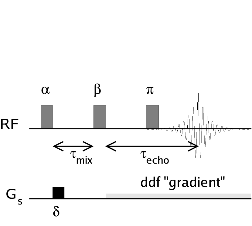
Figure 14.1: The HOMOGENIZED pulse sequence.

The sequence shown in Figure 14.1 consists of three RF pulses, $\alpha$ for excitation, $\beta$ to convert helical transverse magnetization to $M_{z}$ modulation, and $\pi$ to form a spin-echo. The $G_{s}$ gradient in combination with $\beta$ creates spatially-modulated longitudinal magnetization whose magnetic field causes unwinding (and eventually rewinding) of helically twisted transverse magnetization [115].

The goal of the HOMOGENIZED sequence is to obtain a high resolution 1d spectrum by performing a 2d acquisition and projecting along the $F2$ dimension.

14.3 Step by Step HOMOGENIZED

It is helpful to visualize the HOMOGENIZED sequence in a step by step manner, noting analogies to more commonly understood spin behavior. The process is twofold, first, noting when the sequence does not utilize the DDF and so behaves as conventionally expected, and second, noting when the sequence utilizes the DDF and how the behavior departs from commonly understood behavior. We will also note simplifying assumptions that have been made along the way. The following description is done in the rotating frame of the solvent $S$.

14.3.1 Excitation by the $\alpha$ pulse

First, the HOMOGENIZED sequence excites the system with the $\alpha$ pulse. This will usually be a $90^{\circ}$ pulse, unless utilizing a short $TR$ in which case one might use the Ernst angle (see section 4.1.1). We will use a non-selective $90^{\circ}$, phase $\phi_{\alpha}$, “hard” pulse, although variations of HOMOGENIZED have used selective pulses [89]. We start with fully relaxed magnetization, with two spin types $I$ and $S$. After the $\alpha$ pulse we have, using the longitudinal/transverse notation,

$$M_{\perp}^{\alpha}=i\,[M_{0}^{I}+M_{0}^{S}]\,e^{i\,\phi_{\alpha}},$$ (14.1)

and

$$M_{\parallel}^{\alpha}=0.$$ (14.2)

This is for a homonuclear system where the hard pulse has bandwidth to cover both $I$ and $S$ magnetization.

14.3.2 $G_{s}$gradient

The $G_{s}$ gradient of duration $\delta$ causes the transverse magnetization to “twist” along the $\hat{s}$ spatial direction. The pitch of the twist is

$$q=\frac{\gamma}{2\pi}G_{s}\delta.$$ (14.3)

After the applied gradient we have

$$M_{\perp}^{G}=i\,[M_{0}^{I}+M_{0}^{S}]\,e^{i\,\phi_{\alpha}-i\,2\pi\,q\,s},$$ (14.4)

and

$$M_{\parallel}^{G}=0.$$ (14.5)

14.3.3 $\tau_{mix}$ delay

During the $\tau_{mix}$delay (which includes $\delta$) we will have phase “evolution” of transverse magnetization due to resonance offsets, in this case the chemical shift. We will assume that the $S$ magnetization is on-resonance and that there is a chemical shift of $I$ relative to $S$ of $\sigma$. We will neglect other effects such as field inhomogeneity, relaxation, and diffusion for now. This gives us

$$M_{\perp}^{\tau_{mix}}=i\,[M_{0}^{I}e^{i\,\sigma\,\omega_{0}\tau_{mix}}+M_{0}^{S}]\,e^{i\,\phi_{\alpha}-i\,2\pi\,q\,s},$$ (14.6)

and

$$M_{\parallel}^{\tau_{mix}}=0.$$ (14.7)

We will assume that $\sigma$ is large enough to meet the condition

$$\frac{\sigma\,\omega_{0}}{2\pi}\gg\frac{1}{\tau_{d}}$$ (14.8)

where $\tau_{d}$, defined in section 12.2, is the timescale it takes the DDF to cause significant precession of magnetization. $\tau_{d}$ needs to be computed from the sum of both $S$ and $I$ magnetizations when both are significant. The condition states that the chemical shift will dephase or average to zero any DDF component originating from transverse magnetization. As a practical guide, the $I$ and $S$ peaks in the spectrum should not significantly overlap due to inhomogeneous broadening ($T_{2}$relaxation) for this condition to be met.

14.3.4 $\beta$ pulse

The purpose of the $\beta$ pulse is to form spatially-modulated longitudinal magnetization from the “twisted” transverse magnetization. $\beta$ is again assumed to be a “hard” pulse with sufficient bandwidth to cover both $I$ and $S$ resonance offsets.

The flip angle of $\beta$ controls the “depth” or magnitude of the modulation. We will see that different flip angles for $\beta$ can lead to different classes of signals being optimized at the end of the sequence.

We will look at the case where $\beta$ has phase $-\hat{y}$ or $\phi_{\beta}=-\frac{\pi}{2}$. We now have

$$M_{\perp}^{\beta}=i\,M_{0}^{I}cos(\phi_{\alpha}+\tau_{mix}\sigma\,\omega_{0}-2\pi\,q\,s)-M_{0}^{I}sin(\phi_{\alpha}+\tau_{mix}\sigma\,\omega_{0}-2\pi\,q\,s)\,cos(\beta)\\ +i\,M_{0}^{S}cos(\phi_{\alpha}-2\pi\,q\,s)-M_{0}^{S}sin(\phi_{\alpha}-2\pi\,q\,s)\,cos(\beta)$$ (14.9)

and

$$M_{\parallel}^{\beta}=-M_{0}^{I}sin(\phi_{\alpha}+\tau_{mix}\sigma\,\omega_{0}-2\pi\,q\,s)\,sin(\beta)-M_{0}^{S}sin(\phi_{\alpha}-2\pi\,q\,s)\,sin(\beta).$$ (14.10)

We notice immediately that the longitudinal component amplitude is maximized when $\beta=\frac{\pi}{2}$ or $\frac{3\pi}{2}$. The real ($\hat{x}$) transverse component is concomitantly minimized. Both transverse and longitudinal components have spatial variation (modulation) due to the gradient, and chemical shift variation is present for the $I$ magnetization.

14.3.5 $\frac{\tau_{echo}}{2}$ Delay

The $\tau_{echo}$ delay is split in half by the $\pi$ RF pulse, forming a spin-echo. During the first half of the delay period $\frac{\tau_{echo}}{2}$ we will again have chemical shift evolution, but this will be refocused at the spin echo point. Since we now have longitudinal magnetization, we will have a DDF. This DDF is not averaged away by off-resonance effects as described in section 14.3.3.

We restate (from section 12.3 equations 12.13 and 12.14) the Bloch equations for the DDF in transverse and longitudinal form

$$\frac{dM_{\perp}^{I}(\vec{r})}{dt}=-i\,\gamma_{I}\,\mu_{0}\Lambda(\hat{s})\,[M_{\parallel}^{I}(\vec{r})\,M_{\perp}^{I}(\vec{r})+\frac{1}{3}M_{\perp}^{S}(\vec{r})\,M_{\parallel}^{I}(\vec{r})+\frac{2}{3}M_{\parallel}^{S}(\vec{r})\,M_{\perp}^{I}(\vec{r})]+i\,\Delta\omega_{0}^{I}\,M_{\perp}^{I}(\vec{r}),$$ (14.11)

and

$$\frac{dM_{\parallel}^{I}(\vec{r})}{dt}=i\,\gamma_{I}\,\mu_{0}\Lambda(\hat{s})\,[\frac{1}{6}M_{\perp}^{S}(\vec{r})\,\{M_{\perp}^{I}(\vec{r})\}^{\star}-\frac{1}{6}\{M_{\perp}^{S}(\vec{r})\}^{\star}\,M_{\perp}^{I}(\vec{r})].$$ (14.12)

We assume that the condition 14.3.3

$$\frac{\sigma\,\omega_{0}}{2\pi}\gg\frac{1}{\tau_{d}}$$ (14.13)

is met, which leads to any transverse “field” term (the left term in each pair of magnetization products) that is off-resonance giving a time average DDF of zero. This simplifies the equations to

$$\frac{dM_{\perp}^{I}(\vec{r})}{dt}=-i\,\gamma_{I}\,\mu_{0}\Lambda(\hat{s})\,[M_{\parallel}^{I}(\vec{r})\,M_{\perp}^{I}(\vec{r})+\frac{2}{3}M_{\parallel}^{S}(\vec{r})\,M_{\perp}^{I}(\vec{r})]-i\,\Delta\omega_{0}^{I}\,M_{\perp}^{I}(\vec{r}),$$ (14.14)

and

$$\frac{dM_{\parallel}^{I}(\vec{r})}{dt}=0$$ (14.15)

We now have again no change in the longitudinal component due to the DDF, similar to the single component system (equation 12.7).

We use the following notation for the DDF, which is subtly different than that introduced in equation 12.12. This is the total DDF “felt” by the $I$ magnetization, not the DDF due to $I$ magnetization alone,

$$B_{d,\,I}(\vec{r})=\mu_{0}\Lambda(\hat{s})\,[M_{\parallel}^{I}(\vec{r})+\frac{2}{3}M_{\parallel}^{S}(\vec{r})].$$ (14.16)

It is a longitudinal field only, and does not change due to DDF or off-resonance effects . Substituting 14.16 into 14.14 gives

$$\frac{dM_{\perp}^{I}(\vec{r})}{dt}=-i\,[\gamma_{I}B_{d,\,I}(\vec{r})-\Delta\omega_{0}^{I}]\,M_{\perp}^{I}(\vec{r})$$ (14.17)

This represents transverse $I$ magnetization precessing due to resonance offset and a spatially dependent longitudinal field (like a gradient). It has the solution

$$M_{\perp}^{I}(\vec{r})=M_{\perp,\,0}^{I}(\vec{r})\,e^{-i\,[\gamma_{I}B_{d,\,I}(\vec{r})-\Delta\omega_{0}^{I}]\,t}$$

We can get similar expressions for $S$ by exchanging $I$ and $S$.

We now have, after the $\frac{\tau_{echo}}{2}$ portion of the HOMOGENIZED sequence, the magnetization states

$$M_{\perp}^{\frac{\tau_{echo}}{2}}=M_{0}^{I}[i\,cos(\phi_{\alpha}+\tau_{mix}\sigma\,\omega_{0}-2\pi\,q\,s)\\ -sin(\phi_{\alpha}+\tau_{mix}\sigma\,\omega_{0}-2\pi\,q\,s)\,cos(\beta)]\,e^{-i\,[\gamma_{I}B_{d,\,I}(\vec{r})-\sigma\,\omega_{0}]\,\frac{\tau_{echo}}{2}}\\ +M_{0}^{S}[i\,cos(\phi_{\alpha}-2\pi\,q\,s)-sin(\phi_{\alpha}-2\pi\,q\,s)\,cos(\beta)]\,e^{-i\,\gamma_{S}B_{d,\,S}(\vec{r})\,\frac{\tau_{echo}}{2}}$$ (14.18)

and

$$M_{\parallel}^{\frac{\tau_{echo}}{2}}=-M_{0}^{I}sin(\phi_{\alpha}+\tau_{mix}\sigma\,\omega_{0}-2\pi\,q\,s)\,sin(\beta)-M_{0}^{S}sin(\phi_{\alpha}-2\pi\,q\,s)\,sin(\beta).$$ (14.19)

We have made the substitution $\sigma\,\omega_{0}=\Delta\omega_{0}$ in equation 14.18.

14.3.6 $\pi$ pulse and spin echo

We will simplify the effects of the $\pi$ pulse by fixing its flip angle ( to $180^{\circ}$) and phase to $-\hat{y}$. This inverts the longitudinal magnetization and inverts the $\hat{x}$ component of the transverse magnetization. We have

$$M_{\perp}^{\pi}=M_{0}^{I}[i\,cos(\phi_{\alpha}+\tau_{mix}\sigma\,\omega_{0}-2\pi\,q\,s)\\ +sin(\phi_{\alpha}+\tau_{mix}\sigma\,\omega_{0}-2\pi\,q\,s)\,cos(\beta)]\,e^{-i\,[\gamma_{I}B_{d,\,I}(\vec{r})-\sigma\,\omega_{0}]\,\frac{\tau_{echo}}{2}}\\ +M_{0}^{S}[i\,cos(\phi_{\alpha}-2\pi\,q\,s)+sin(\phi_{\alpha}-2\pi\,q\,s)\,cos(\beta)]\,e^{-i\,\gamma_{S}B_{d,\,S}(\vec{r})\,\frac{\tau_{echo}}{2}}$$ (14.20)

and

$$M_{\parallel}^{\pi}=M_{0}^{I}sin(\phi_{\alpha}+\tau_{mix}\sigma\,\omega_{0}-2\pi\,q\,s)\,sin(\beta)+M_{0}^{S}sin(\phi_{\alpha}-2\pi\,q\,s)\,sin(\beta).$$ (14.21)

14.3.7 Second $\frac{\tau_{echo}}{2}$ Delay

The second $\frac{\tau_{echo}}{2}$ is similar to the first. At the echo point the chemical shift is refocused. The DDF-induced phase is not canceled since the longitudinal magnetization causing the DDF has been inverted as well. We end up with

$$M_{\perp}^{\tau_{echo}}=M_{0}^{I}[i\,cos(\phi_{\alpha}+\tau_{mix}\sigma\,\omega_{0}-2\pi\,q\,s)\\ +sin(\phi_{\alpha}+\tau_{mix}\sigma\,\omega_{0}-2\pi\,q\,s)\,cos(\beta)]\,e^{-i\,\gamma_{I}B_{d,\,I}(\vec{r})\,\tau_{echo}}\\ +M_{0}^{S}[i\,cos(\phi_{\alpha}-2\pi\,q\,s)+sin(\phi_{\alpha}-2\pi\,q\,s)\,cos(\beta)]\,e^{-i\,\gamma_{S}B_{d,\,S}(\vec{r})\,\tau_{echo}}$$ (14.22)

and

$$M_{\parallel}^{\tau_{echo}}=M_{0}^{I}sin(\phi_{\alpha}+\tau_{mix}\sigma\,\omega_{0}-2\pi\,q\,s)\,sin(\beta)+M_{0}^{S}sin(\phi_{\alpha}-2\pi\,q\,s)\,sin(\beta).$$ (14.23)

14.4 Signal growth due to the DDF

The spatially-varying longitudinal DDF will alter the phase of the transverse magnetization, which also has spatial variation. At this point we will make the simplifying assumption that all spatial variation is due to the applied gradient. We will also conduct the analysis first for transverse $I$ magnetization.

The $I$ transverse magnetization is

$$M_{\perp}^{I}=M_{0}^{I}[i\,cos(\phi_{\alpha}+\tau_{mix}\sigma\,\omega_{0}-2\pi\,q\,s)\\ +sin(\phi_{\alpha}+\tau_{mix}\sigma\,\omega_{0}-2\pi\,q\,s)\,cos(\beta)]\,e^{-i\,\gamma_{I}B_{d,\,I}(\vec{r})\,t+i\,\sigma\,\omega_{0}(t-\tau_{echo})},$$ (14.24)

for the time period $t$ after the $\beta$ pulse. We have taken the final form of the magnetization after the $\pi$ pulse. Substituting 15.17 into 14.16 gives

$$B_{d,\,I}(\vec{r})=\mu_{0}\Lambda(\hat{s})\,[M_{0}^{I}sin(\phi_{\alpha}+\tau_{mix}\sigma\,\omega_{0}-2\pi\,q\,s)\,sin(\beta)+\frac{2}{3}M_{0}^{S}sin(\phi_{\alpha}-2\pi\,q\,s)\,sin(\beta)].$$ (14.25)

We make the following substitutions

$$x_{I}=\phi_{\alpha}+\sigma\,\omega_{0}\tau_{mix}-2\pi\,q\,s,$$ (14.26)

$$x_{S}=\phi_{\alpha}-2\pi\,q\,s,$$ (14.27)

$$z_{I}=\gamma_{I}\mu_{0}\Lambda(\hat{s})\,M_{0}^{I}sin(\beta)\,t,$$ (14.28)

and

$$z_{S}=\frac{2}{3}\gamma_{I}\mu_{0}\Lambda(\hat{s})\,M_{0}^{S}sin(\beta)\,t$$ (14.29)

where $x$ and $z$ are variables of convenience only, and do not designate coordinates or directions. Substitution into 14.25 and 14.24 gives us

$$M_{\perp}^{I}=M_{0}^{I}[i\,cos(x_{I})+sin(x_{I})\,cos(\beta)]\,e^{i\,\sigma\,\omega_{0}(t-\tau_{echo})}e^{i\,z_{I}sin(x_{I})}e^{i\,z_{S}sin(x_{S})}.$$ (14.30)

Now we use a form of the generating function for Bessel functions

$$e^{i\,z\,sin(x)}=\sum_{m=-\infty}^{\infty}e^{i\,m\,x}J_{m}(z),$$ (14.31)

which is obtained by substituting $cos(x-\frac{\pi}{2})=sin(x)$ into [117, 8.511 4. p973]

$$e^{i\,z\,cos(x)}=\sum_{m=-\infty}^{\infty}i^{m}e^{i\,m\,x}J_{m}(z).$$ (14.32)

Substitution of 14.31 into 14.30 gives

$$M_{\perp}^{I}=M_{0}^{I}[i\,cos(x_{I})-sin(x_{I})\,cos(\beta)]\,e^{i\,\sigma\,\omega_{0}(t-\tau_{echo})}\sum_{m=-\infty}^{\infty}\sum_{n=-\infty}^{\infty}e^{i\,m\,x_{I}}e^{i\,n\,x_{S}}J_{m}(z_{I})J_{n}(z_{S}).$$ (14.33)

The detected signal amplitude in magnetic resonance is proportional to the spatial integral of the transverse magnetization over the sample

$$A\propto\int_{sample}M_{\perp}(\vec{r})\,d^{3}r.$$ (14.34)

The proportionality relation takes into account the coil sensitivity and amplifier gain.

The only terms in the double sum of equation 14.33 that will lead to significant signal are those that have no spatial variation (are not spoiled). The spatial variation is found in the $-2\pi\,q\,s$ terms of $x_{I}$ and $x_{s}$. We can therefore search for terms where $x_{I}$ and $x_{S}$ cancel in the exponent. We must take into account the $cos(x_{I})$ and $sin(x_{I})$ terms in front as well. We make the substitutions

$$cos(x)=\frac{e^{i\,x}+e^{-i\,x}}{2}$$ (14.35)

and

$$sin(x)=-i\frac{e^{i\,x}-e^{-i\,x}}{2}$$ (14.36)

into 14.33, which yields

$$M_{\perp}^{I}=i\,M_{0}^{I}[\frac{e^{i\,x_{I}}+e^{-i\,x_{I}}}{2}-\frac{e^{i\,x_{I}}-e^{-i\,x_{I}}}{2}cos(\beta)]\\ e^{i\,\sigma\,\omega_{0}(t-\tau_{echo})}\sum_{m=-\infty}^{\infty}\sum_{n=-\infty}^{\infty}e^{i\,m\,x_{I}}e^{i\,n\,x_{S}}J_{m}(z_{I})\,J_{n}(z_{S}).$$ (14.37)

There are two cases where the net $x$ power is zero (note that $x_{S}$ is equivalent to $x_{I}$ for spatial dependence $-2\,q\,s$),

$$n=-(m-1)$$ (14.38)

and

$$n=-(m+1).$$ (14.39)

We separate these two classes of terms to get

$$M_{\perp p}^{I}=\frac{1}{2}i\,M_{0}^{I}[1+cos(\beta)]e^{i\,\sigma\,\omega_{0}(t-\tau_{echo})}\sum_{m=-\infty}^{\infty}e^{i\,(m+1)\,x_{I}}e^{-i\,(m+1)\,x_{S}}J_{m}(z_{I})\,J_{-(m+1)}(z_{S})$$ (14.40)

and

$$M_{\perp n}^{I}=\frac{1}{2}i\,M_{0}^{I}[1-cos(\beta)]e^{i\,\sigma\,\omega_{0}(t-\tau_{echo})}\sum_{m=-\infty}^{\infty}e^{i\,(m-1)\,x_{I}}e^{-i\,(m-1)\,x_{S}}J_{m}(z_{I})\,J_{-(m-1)}(z_{S}).$$ (14.41)

finally we can substitute back our values of $x$ and $z$ to get

$$M_{\perp p}^{I}=\frac{1}{2}i\,M_{0}^{I}[1+cos(\beta)]\,e^{i\,\sigma\,\omega_{0}(t-\tau_{echo})}\\ \sum_{m=-\infty}^{\infty}e^{i\,(m+1)\,\sigma\,\omega_{0}\tau_{mix}}J_{m}[\gamma_{I}\mu_{0}\Lambda(\hat{s})\,M_{0}^{I}sin(\beta)\,t]\,J_{-(m+1)}[\frac{2}{3}\gamma_{I}\mu_{0}\Lambda(\hat{s})\,M_{0}^{S}sin(\beta)\,t]$$ (14.42)

$$M_{\perp n}^{I}=\frac{1}{2}i\,M_{0}^{I}[1-cos(\beta)]\,e^{i\,\sigma\,\omega_{0}(t-\tau_{echo})}\\ \sum_{m=-\infty}^{\infty}e^{i\,(m-1)\,\sigma\,\omega_{0}\tau_{mix}}J_{m}[\gamma_{I}\mu_{0}\Lambda(\hat{s})\,M_{0}^{I}sin(\beta)\,t]\,J_{-(m-1)}[\frac{2}{3}\gamma_{I}\mu_{0}\Lambda(\hat{s})\,M_{0}^{S}sin(\beta)\,t]$$ (14.43)

We can make two more substitutions

$$\tau_{dII}=\frac{1}{\gamma_{I}\,\mu_{0}M_{0}^{I}}$$ (14.44)

and

$$\tau_{dIS}=\frac{1}{\gamma_{I}\,\mu_{0}M_{0}^{S}}$$ (14.45)

to get

$$M_{\perp p}^{I}=\frac{1}{2}i\,M_{0}^{I}[1+cos(\beta)]\,e^{i\,\sigma\,\omega_{0}(t-\tau_{echo})}\\ \sum_{m=-\infty}^{\infty}e^{i\,(m+1)\,\sigma\,\omega_{0}\tau_{mix}}J_{m}[\Lambda(\hat{s})\,sin(\beta)\frac{t}{\tau_{dII}}]\,J_{-(m+1)}[\frac{2}{3}\Lambda(\hat{s})\,sin(\beta)\frac{t}{\tau_{dIS}}]$$ (14.46)

and

$$M_{\perp n}^{I}=\frac{1}{2}i\,M_{0}^{I}[1-cos(\beta)]\,e^{i\,\sigma\,\omega_{0}(t-\tau_{echo})}\\ \sum_{m=-\infty}^{\infty}e^{i\,(m-1)\,\sigma\,\omega_{0}\tau_{mix}}J_{m}[\Lambda(\hat{s})\,sin(\beta)\frac{t}{\tau_{dII}}]\,J_{-(m-1)}[\frac{2}{3}\Lambda(\hat{s})\,sin(\beta)\frac{t}{\tau_{dIS}}].$$ (14.47)

The results for $S$ ( obtained by interchanging $I$ and $S$ in equations 14.40 and 14.41) are

$$M_{\perp p}^{S}=\frac{1}{2}i\,M_{0}^{S}[1+cos(\beta)]\\ \sum_{m=-\infty}^{\infty}e^{-i\,(m+1)\,\sigma\,\omega_{0}\tau_{mix}}J_{m}[\Lambda(\hat{s})\,sin(\beta)\frac{t}{\tau_{dSS}}]\,J_{-(m+1)}[\frac{2}{3}\Lambda(\hat{s})\,sin(\beta)\frac{t}{\tau_{dSI}}]$$ (14.48)

and

$$M_{\perp n}^{S}=\frac{1}{2}i\,M_{0}^{S}[1-cos(\beta)]\\ \sum_{m=-\infty}^{\infty}e^{-i\,(m-1)\,\sigma\,\omega_{0}\tau_{mix}}J_{m}[\Lambda(\hat{s})\,sin(\beta)\frac{t}{\tau_{dSS}}]\,J_{-(m-1)}[\frac{2}{3}\Lambda(\hat{s})\,sin(\beta)\frac{t}{\tau_{dSI}}].$$ (14.49)

Note that the phase of the $\alpha$ RF pulse $\phi_{\alpha}$ has dropped out of the equations through cancellation.

14.5 Interpreting the results

The equations 14.46 and 14.47 lead to a series of peaks in a two dimensional spectrum. The $e^{i\,\sigma\,\omega_{0}(t-\tau_{echo})}$ term causes the shift in the directly detected $F_{2}$ dimension. This term is missing from the $S$ magnetization which for simplicity was made on resonance. Performing multiple acquisitions while incrementing $\tau_{mix}$ provides the indirect, or $F_{1}$ dimension. The shift in the $F_{1}$ dimension is determined by the $e^{i\,(m-1)\,\sigma\,\omega_{0}\tau_{mix}}$and similar terms.

There are theoretically an infinite number of peaks (which could alias along the $F_{1}$ dimension) of each type $p$ or $n$ but in practice relaxation will limit the number of peaks observed. Also the relative concentration of $S$ and $I$ will limit the number, the largest number of peaks observed when $S$ and $I$ magnetizations are in the ratio 1 to 1 [116]. Those peaks corresponding to the lowest order Bessel functions are most easily observed, as they build the fastest, before relaxation and diffusion effects can attenuate the signal. For example, if the $I$ spin is present in low concentration, only the term $J_{0}[\Lambda(\hat{s})\,sin(\beta)\frac{t}{\tau_{dII}}]$ corresponding to $m=0$ will have significant amplitude for the $M^{I}$ cross peaks. We summarize in figure 14.3 with a corresponding experimental example in figure 14.2.

Figures 14.4, 14.5 and 14.6 show the temporal behavior of relative peak amplitudes for specific cases. For the case of $\beta=\pm 45^{\circ}$the $p$-type crosspeak magnitude is maximized, and for $\beta=\pm 135^{\circ}$ the $n$ type crosspeak magnitude is maximized.

We can think of the terms of the type $\Lambda(\hat{s})\,sin(\beta)\frac{\tau_{echo}}{\tau_{dII}}$ inside the Bessel function in equations 14.46, 14.47, etc. as a linear time proportional “unwinding” parameter, which depends on field, concentration, and $\gamma$ (through $M_{0})$, the flip angles (only $\beta$ in this case) and on the applied gradient angle (through $\Lambda(\hat{s})$).

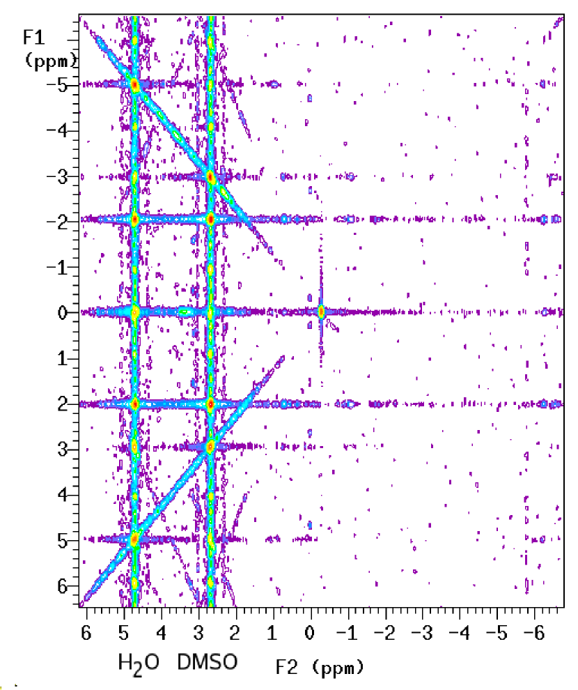
Figure 14.2: Example HOMOGENIZED spectrum of 50% $H_{2}O$ (4.8 ppm) and 50% $DMSO$ (2.8 ppm) at 4 Tesla. $F_{2}$ resolution is 1024 points, $F_{1}$ resolution 256 points. $\beta=90^{\circ}$ yields symmetry along $F_{1}$. The diagonal lines and peaks that lie on them are incompletely spoiled magnetization “artifacts”. Vertical lines are the magnitude tails as well as“T1” noise which results from slight phase errors of pulses and incomplete crushing. Horizontal lines are magnitude tails along $F_{2}$ and “zero quantum” noise.

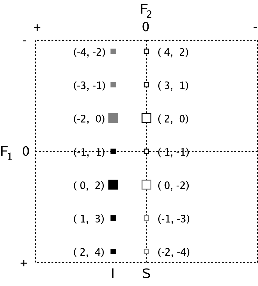
Figure 14.3: Schematic 2d HOMOGENIZED spectrum - Cross peaks are labeled as $(m_{p},\,m_{n})$. The dominant peaks (with $m_{p}$or $m_{n}=0$) are shown as large squares. Peaks with major contribution of $p$ type for spin $I$ are filled in black. $n$ type peaks are shown as solid gray. Peaks corresponding to $m\neq 0$ are small squares. For spin $S$ the peaks are not filled.

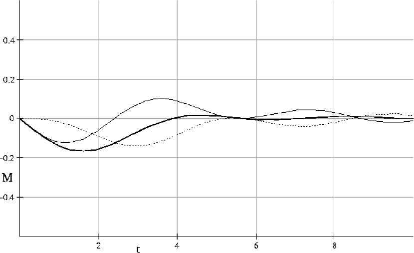
Figure 14.4: $I$ peak amplitude for $(m_{p},\,m_{n})=(0,\,2)$, $\beta=\frac{\pi}{2}$, $M_{0}^{S}=1.0$, $M_{0}^{I}=1.0$. The time scale is arbitrary. The heavy curve is the sum of the $p$ and $n$ type contributions (net peak amplitude). The normal curve is the $p$ type contribution. The dotted curve is the $n$ type contribution. At short times this peak is dominated by the $p$ type signal.

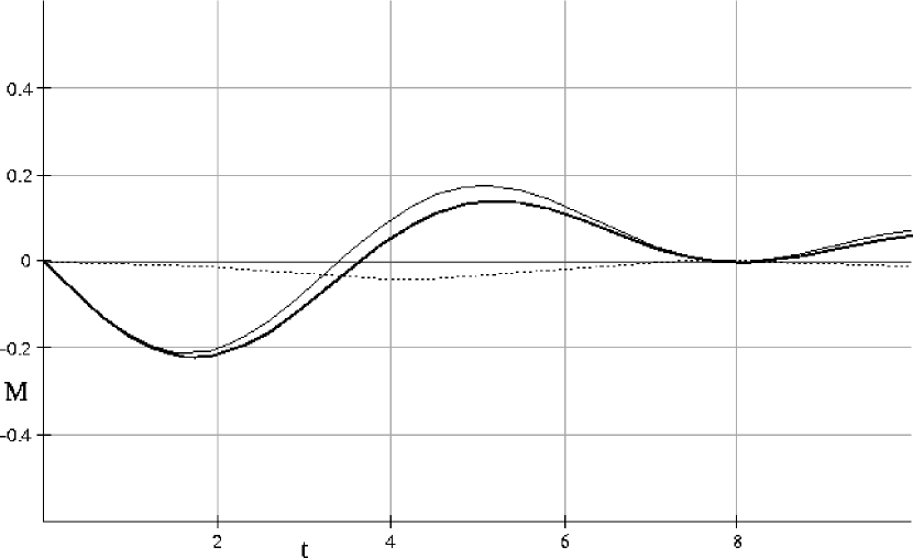
Figure 14.5: $I$ peak amplitude for $(m_{p},\,m_{n})=(0,\,2)$, $\beta=\frac{\pi}{4}$, $M_{0}^{S}=1.0$, $M_{0}^{I}=1.0$. Same labeling as in figure 14.4. Changing $\beta$ has increased the $p$ type contribution in this peak and decreased the $n$ type, raising the overall maximum amplitude.

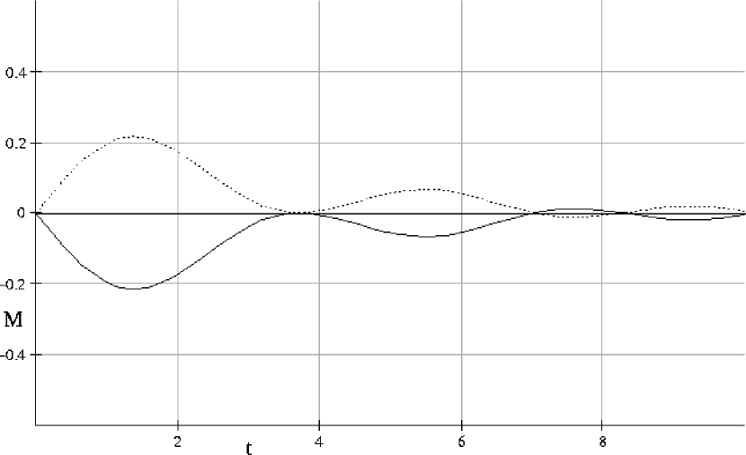
Figure 14.6: $I$ peak amplitude for $(m_{p},\,m_{n})=(-1,\,1)$, $\beta=\frac{\pi}{2}$, $M_{0}^{S}=1.0$, $M_{0}^{I}=1.0$. Same labeling as in figure 14.4. This is a so called “axial” peak. The $p$ and $n$ type contributions cancel for $\beta=\frac{\pi}{2}$.

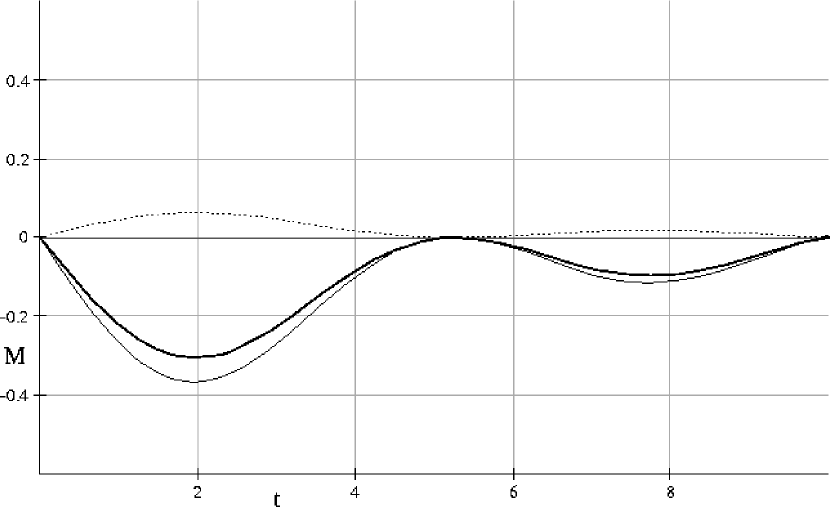
Figure 14.7: $I$ peak amplitude for $(m_{p},\,m_{n})=(-1,\,1)$, $\beta=\frac{\pi}{4}$, $M_{0}^{S}=1.0$, $M_{0}^{I}=1.0$. Same labeling as in figure 14.4. This axial peak can have non-zero amplitude even when the concentration of $S$ spins is zero, due to $I,\,I$ spin interaction.

14.6 Why HOMOGENIZED homogenizes…

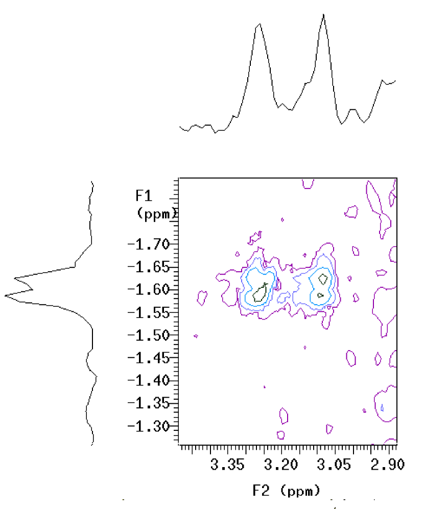
Figure 14.8: HOMOGENIZED spectrum of 99.9% $H_{2}O$ (2.8 ppm) and ~20 mM Choline Chloride (3.2 ppm) at 4 Tesla, showing the region around the (0, 2) Choline peak. $F_{2}$ resolution is 1024 points, $F_{1}$ resolution 512 points. The $X$ shim has been deliberately offset to give a very broad line in the $F_{2}$ projection. It has actually split the peak into two peaks (for unknown reasons, possibly spoiling during acquisition). The $F_{1}$projection peak is much narrower.

The HOMOGENIZED signal results from refocusing due to the DDF. As long as the DDF has not been perturbed significantly by any susceptibility or inhomogeneity fields (during the $\tau_{mix}$ period) there will not be significant broadening of the chemical shifts in the $F1$ dimension. This is not true of the $F2$ dimension, and we still have $T_{2}^{*}$ effects determining the SNR of the acquired FID.

The condition can be stated as follows

$$\Delta B\,\tau_{mix}\ll G\,\delta\,\Delta s,$$

where $\Delta B\,\tau_{mix}$ is the total magnitude of field inhomogeneity over the sample acting over the mixing time, and $G\,\delta\,\Delta s$ is the HOMOGENIZED gradient strength duration product multiplied by the dimension of the sample. This condition means that the modulation pattern is undisturbed by inhomogeneity.

Another way of looking at this effect is to say that only the inhomogeneity on the scale of $q$ (see equation 15.3) matters, and that HOMOGENIZED “shrinks” the sample down to size $q$.

We show an example in figure 14.8.

Chapter 15 HOMOGENIZED WITH $T_{2}$ RELAXATION AND DIFFUSION

15.1 Introduction

An analytical expression, equation (15.20), for the HOMOGENIZED cross peak amplitude in the presence of diffusion and $T_{2}$ relaxation has been developed.

HOMOGENIZED [2] and its variants [89, 120] and the recently proposed IDEAL [90] sequences have great potential for in-vivo magnetic resonance spectroscopy [86] (MRS). Diffusion weighting in HOMOGENIZED is present both to give intentional diffusion weighting and as a side effect of the various gradients present. Stejskal-Tanner (ST) diffusion weighting [53] during the $\tau_{mix}$ and $\tau_{echo}$ periods of the sequence can also be used to suppress radiation dampening. “Enhanced” diffusion weighting [121, 122, 123] is obtained by reducing the DDF during $\tau_{echo}$. There is an additional $\tau_{echo}$ dependent diffusion weighting possible, due to the iZQC (intermolecular zero quantum coherence) gradient $G_{zq}$ and $\beta$ pulse combination. The weighting results from diffusing modulated longitudinal magnetization. Kennedy et al. [1] have shown recently that this diffusion weighting has the novel property of being insensitive to object motion. $T_{2}$ relaxation also attenuates the signal.

It is desirable to have an analytical signal equation describing HOMOGENIZED cross peaks. This is a necessary first step to using HOMOGENIZED for quantitative in-vitro and in-vivo spectroscopy.

15.2 Step by Step HOMOGENIZED with $T_{2}$ Relaxation and Diffusion

We will concentrate our discussion on the 2d HOMOGENIZED sequence shown in figure 15.1. This sequence is very similar to the HOMOGENIZED sequence discussed in chapter 14 and shown in figure 14.1. The difference is that there are several additional gradient pairs to allow control of Stejskal Tanner diffusion weighting during the $\tau_{mix}$ and $\tau_{echo}$ periods and to allow separate control of the diffusion weighting due to $G_{zq}$. We have also added crusher gradients around the $\pi$ RF pulse.

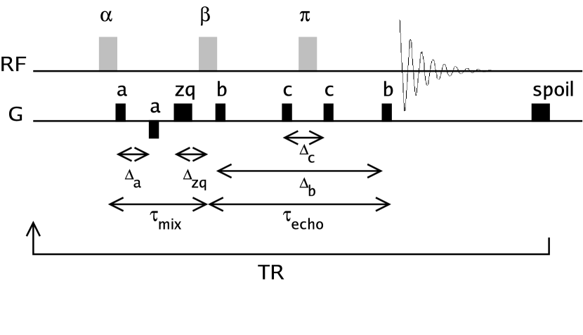
Figure 15.1: HOMOGENIZED pulse sequence with Stejskal-Tanner diffusion weighting during $\tau_{mix}$ and $\tau_{echo}$ and crusher gradients on the $\pi$ RF pulse.

15.2.1 Excitation by the $\alpha$ pulse

First, the HOMOGENIZED sequence excites the system with the $\alpha$ pulse. This is unchanged from section 14.3.1. For simplicity will assume that the system starts fully relaxed, and that we are using $\alpha=90^{\circ}$with phase $\phi_{\alpha}$. One could substitute the steady state values for $M^{I}$ and $M^{S}$ , and consider $\alpha\neq 90^{\circ}$ which will lead to additional effects discussed in chapter 16. The transverse and longitudinal magnetization after the $\alpha$ pulse are

$$M_{\perp}^{\alpha}=i\,[M_{0}^{I}+M_{0}^{S}]\,e^{i\,\phi_{\alpha}},$$ (15.1)

and

$$M_{\parallel}^{\alpha}=0.$$ (15.2)

This is for a homonuclear system where the hard pulse has bandwidth to cover both $I$ and $S$ magnetization.

15.2.2 $G_{a}$ gradients and delay $\Delta_{a}$

Here is the first departure from chapter 14. The first $G_{a}$ is half of a gradient pair designed to give Stejskal-Tanner diffusion weighting to transverse magnetization during a significant portion of the $\tau_{mix}$ time period $\Delta_{a}$. It also serves to keep the transverse magnetization in a spoiled state to reduce radiation damping effects.

The first $G_{a}$ gradient of duration $\delta_{a}$ and direction $\hat{s}_{a}$results in

$$q=\frac{\gamma}{2\pi}G_{a}\delta_{a}$$ (15.3)

for both $I$ and $S$ magnetization. The second $G_{a}$ gradient has the same duration $\delta_{a}$ and opposite magnitude, refocusing the magnetization giving $q=0$. The combined effects of the $G_{a}$ gradients and $\Delta_{a}$ delay is Stejskal-Tanner diffusion weighting as discussed in section 10.1. The $b-value$ for this diffusion weighting is

$$b_{a}=\gamma^{2}G_{a}^{2}\delta_{a}^{2}(\Delta_{a}-\frac{\delta_{a}}{3}).$$ (15.4)

15.2.3 $G_{zq}$ gradient

The $G_{zq}$ gradient (applied along direction $\hat{s}_{zq}$) has multiple effects. It selects the desired zero-quantum coherence pathway during $\tau_{mix}$ by twisting transverse magnetization, and ensuring that only untwisting by the DDF (Distant Dipolar Field) leads to observable signal at the end of the sequence. The $G_{zq}$ gradient also introduces diffusion weighting. Finally it determines the spatial scale (correlation distance) of the DDF as discussed in section 11.4.

The diffusion weighting $b-value$ from $G_{zq}$ up until the $\beta$ pulse (duration $\Delta_{zq}$) is of the Stejskal-Tanner type, but we omit the final gradient contribution (see table 10.1)

$$b_{zq}=\gamma^{2}G_{zq}^{2}\delta_{zq}^{2}(\Delta_{zq}-\frac{2\,\delta_{zq}}{3}).$$ (15.5)

The spatial frequency $q_{zq}$ of transverse magnetization is now

$$q_{zq}=\frac{\gamma}{2\pi}G_{zq}\delta_{zq}.$$ (15.6)

15.2.4 $\tau_{mix}$ time period

The $\tau_{mix}$ time period is inclusive of the $G_{a}$ gradient pair, $G_{zq}$ gradient and their associated delays. We assume that the duration of the $\alpha$ and $\beta$ RF pulses is short compared to the other delays, and include half of each pulse duration in $\tau_{mix}$. During these pulses and delays there is also $T_{2}$ relaxation (and $T_{1}$ relaxation which we will neglect). We can now write the transverse magnetization state immediately before the $\beta$ RF pulse

$$M_{\perp}^{\tau_{mix}}=i\,e^{i\,\phi_{\alpha}}e^{-i\,2\,\pi\,q_{zq}\,s_{zq}}[M_{0}^{I}e^{i\,\omega_{0}\sigma\,\tau_{mix}}e^{-(b_{a}+b_{zq})\,D^{I}}e^{-\frac{\tau_{mix}}{T_{2}^{I}}}+M_{0}^{S}e^{-(b_{a}+b_{zq})\,D^{S}}e^{-\frac{\tau_{mix}}{T_{2}^{S}}}].$$ (15.7)

$T_{2}$ is labeled similarly for each spin type. $\sigma$ is the chemical shift difference.

We have

$$M_{\parallel}^{\tau_{mix}}=0$$ (15.8)

for the longitudinal magnetization state, which is a valid approximation when $\tau_{mix}\ll T_{1}.$

$D$ is the (isotropic) diffusion coefficient, labeled with a superscript for each spin type.

15.2.5 $\beta$ Pulse

The $\beta$ pulse forms modulated longitudinal magnetization, creating a net DDF which will refocus twisted magnetization during $\tau_{echo}$. Immediately after the $\beta$ pulse of phase $\phi_{\beta}=-90^{\circ}$ or $-\hat{y}$ (which is considered to have $\leavevmode\nobreak\ 0$ duration) we have

$$M_{\perp}^{\beta}=i\,M_{0}^{I}cos(\phi_{\alpha}+\tau_{mix}\sigma\,\omega_{0}-2\pi\,q_{zq}\,s_{zq})\,e^{-(b_{a}+b_{zq})\,D^{I}}e^{-\frac{\tau_{mix}}{T_{2}^{I}}}\\ -M_{0}^{I}sin(\phi_{\alpha}+\tau_{mix}\sigma\,\omega_{0}-2\pi\,q_{zq}\,s_{zq})\,cos(\beta)\,e^{-(b_{a}+b_{zq})\,D^{I}}e^{-\frac{\tau_{mix}}{T_{2}^{I}}}\\ +i\,M_{0}^{S}cos(\phi_{\alpha}-2\pi\,q_{zq}\,s_{zq})\,e^{-(b_{a}+b_{zq})\,D^{S}}e^{-\frac{\tau_{mix}}{T_{2}^{S}}}\\ -M_{0}^{S}sin(\phi_{\alpha}-2\pi\,q_{zq}\,s_{zq})\,cos(\beta)\,e^{-(b_{a}+b_{zq})\,D^{S}}e^{-\frac{\tau_{mix}}{T_{2}^{S}}}$$ (15.9)

and

$$M_{\parallel}^{\beta}=-M_{0}^{I}sin(\phi_{\alpha}+\tau_{mix}\sigma\,\omega_{0}-2\pi\,q_{zq}s_{zq})\,sin(\beta)\,e^{-(b_{a}+b_{zq})\,D^{I}}e^{-\frac{\tau_{mix}}{T_{2}^{I}}}\\ -M_{0}^{S}sin(\phi_{\alpha}-2\pi\,q_{zq}s_{zq})\,sin(\beta)\,e^{-(b_{a}+b_{zq})\,D^{S}}e^{-\frac{\tau_{mix}}{T_{2}^{S}}}$$ (15.10)

15.2.6 $G_{b}$ gradients, $\Delta_{b}$ delay, $G_{c}$ gradients and $\Delta_{c}$delay

A lot is going on during the $\tau_{echo}$ period, the DDF is beginning to refocus our desired signal. We have $T_{2}$ relaxation of transverse magnetization, $T_{1}$ relaxation of longitudinal magnetization (which we will again neglect), and attenuation due to diffusion for longitudinal and transverse magnetization. For simplicity we will consider only diffusional attenuation, and discuss DDF refocusing and $T_{2}$ relaxation, which are separable, during our discussion of signal build during $\tau_{echo}$ in section 15.2.7.

We make the assumption that the diffusion attenuation due to the presence of the spatially varying DDF field $\vec{B}_{d}$ (which has a spatially varying gradient) is negligible, a point discussed in reference [74, section I].

The diffusion weighting becomes more complicated, as we are now concerned with the longitudinal and transverse components, and we have applied gradients in differing directions. This leads to increasingly complicated expressions for $q$ and $b$.

The longitudinal magnetization is not affected by the $G_{b}$ or $G_{c}$ gradients, and its $q$ stays as $q_{zq}$. We have attenuation due to diffusion, like in the stimulated echo sequence (section 10.2.6), with $b-value$

$$b_{\parallel}=\gamma^{2}G_{zq}^{2}\delta_{zq}^{2}\Delta_{b}.$$ (15.11)

The transverse magnetization is affected by the $G_{b}$and $G_{c}$gradient pairs, and for simplicity we will assume that $\hat{s}_{zq}\bot\hat{s}_{b}\bot\hat{s}_{c}$. In this case the attenuation can be described by independent $b-values$ from each gradient pair

$$b_{\bot}=b_{\bot zq}+b_{\bot b}+b_{\bot c}$$ (15.12)

with

$$b_{\bot zq}=\gamma^{2}G_{zq}^{2}\delta_{zq}^{2}\Delta_{b},$$ (15.13)

$$b_{\bot b}=\gamma^{2}G_{b}^{2}\delta_{b}^{2}(\Delta_{b}-\frac{\delta_{b}}{3}),$$ (15.14)

and

$$b_{\bot c}=\gamma^{2}G_{c}^{2}\delta_{c}^{2}(\Delta_{c}-\frac{\delta_{c}}{3}).$$ (15.15)

Note that we have included the last $\delta_{b}$ time period in $b_{\bot b,\,b}$.

15.2.7 $\tau_{echo}$ and final magnetization components

During the $\tau_{echo}$ time period we have $T_{1}$ relaxation of the longitudinal magnetization (which we will neglect for now), $T_{2}$ relaxation of the transverse magnetization, and the DDF re-phasing of our desired signal. The $\pi$ pulse also has the effect of inverting longitudinal magnetization, and the $x$ component of the transverse magnetization. From chapter 14 we know that the $\pi$ RF pulse does not reverse the signal re-phasing due to the DDF. In addition we have the diffusion weighting discussed in section 15.2.6.

We end up with the following transverse magnetization

$$M_{\perp}^{\tau_{echo}}=i\,M_{0}^{I}cos(\phi_{\alpha}+\tau_{mix}\sigma\,\omega_{0}-2\pi\,q_{zq}\,s_{zq})\,e^{-(b_{a}+b_{zq}+b_{\bot})\,D^{I}}e^{-\frac{\tau_{mix}+\tau_{echo}}{T_{2}^{I}}}\\ +M_{0}^{I}sin(\phi_{\alpha}+\tau_{mix}\sigma\,\omega_{0}-2\pi\,q_{zq}\,s_{zq})\,cos(\beta)\,e^{-(b_{a}+b_{zq}+b_{\bot})\,D^{I}}e^{-\frac{\tau_{mix}+\tau_{echo}}{T_{2}^{I}}}\\ +i\,M_{0}^{S}cos(\phi_{\alpha}-2\pi\,q_{zq}\,s_{zq})\,e^{-(b_{a}+b_{zq}+b_{\bot})\,D^{S}}e^{-\frac{\tau_{mix}+\tau_{echo}}{T_{2}^{S}}}\\ +M_{0}^{S}sin(\phi_{\alpha}-2\pi\,q_{zq}\,s_{zq})\,cos(\beta)\,e^{-(b_{a}+b_{zq}+b_{\bot})\,D^{S}}e^{-\frac{\tau_{mix}+\tau_{echo}}{T_{2}^{S}}}$$ (15.16)

The longitudinal component is

$$M_{\parallel}^{\tau_{echo}}=M_{0}^{I}sin(\phi_{\alpha}+\tau_{mix}\sigma\,\omega_{0}-2\pi\,q_{zq}s_{zq})\,sin(\beta)\,e^{-(b_{a}+b_{zq})\,D^{I}}e^{-\frac{\tau_{mix}}{T_{2}^{I}}}\,e^{-b_{\parallel}D^{I}}\\ +M_{0}^{S}sin(\phi_{\alpha}-2\pi\,q_{zq}s_{zq})\,sin(\beta)\,e^{-(b_{a}+b_{zq})\,D^{S}}e^{-\frac{\tau_{mix}}{T_{2}^{S}}}\,e^{-b_{\parallel}D^{S}}$$ (15.17)

We have explicitly placed $e^{-b_{\parallel}D}$ separately in each term as we will need to consider its value (which attenuates the DDF) throughout the $\tau_{echo}$ period (and subsequent acquisition period $t2$) rather than just its final value.

15.3 Signal

First, in order to obtain an analytical solution for a system of biological interest, we assume that $M_{0}^{I}\ll M_{0}^{S}$. Making this assumption implies that only the DDF due to $M^{S}$ leads to significant refocused signal and we can neglect the DDF due to $M^{I}$. This collapses the sums in equation 14.46 (and similarly for the others) and leads to only the terms with $J_{0}(\Lambda(\hat{s})\,sin(\beta)\frac{t}{\tau_{dII}})\approx 1$ surviving, since $\Lambda(\hat{s})\,sin(\beta)\frac{t}{\tau_{dII}}\approx 0$ when $\tau_{dII}\rightarrow\infty$. Terms of the type $J_{n}(\Lambda(\hat{s})\,sin(\beta)\frac{t}{\tau_{dII}})\approx 0$, for $n\neq 0$.

We can define some more terms that will help us see the effects of diffusion and $T_{2}$ relaxation.

$$\tau_{dIS,\,eff}\equiv\tau_{dIS}e^{(b_{a}+b_{zq})\,D_{S}}e^{\frac{\tau_{mix}}{T_{2}^{S}}}$$ (15.18)

$\tau_{dIS,\,eff}$ (15.18) has been defined to take account of $T_{2}$ and diffusion losses (ST b-values, $b_{a}$ and $b_{zq}$) incurred during $\tau_{mix}$ before $\beta$ beta forms modulated $M_{\parallel}$. $\tau_{dIS}$ is the dipolar demagnetization time for spin $S$ defined in equation 14.45.

$$F_{IS}(\tau_{echo})\equiv\frac{1-e^{-\tau_{echo}\,(2\pi\,q_{zq})^{2}D_{S}}}{\tau_{dIS,\,eff}(2\pi\,q_{zq})^{2}D_{S}}=\frac{1}{\tau_{dIS,\,eff}}\int_{0}^{\tau_{echo}}e^{-t\,(2\pi\,q_{zq})^{2}D_{S}}dt$$ (15.19)

accounts for the decay of longitudinal magnetization (and the DDF) and can be thought of as an exponentially slowing ”unwinding” parameter, instead of the linear time proportional unwinding parameter as discussed in section 14.5 when diffusion is negligible. It is the integral of the exponentially decaying DDF during $\tau_{echo}$.

The expression for the signal amplitude in the presence of diffusion and $T_{2}$ decay is

$$M_{\perp p}^{I}=-i\,M_{0}^{I}[\frac{cos(\beta)+1}{2}]\,e^{i\,\sigma\,\omega_{0}\tau_{mix}}e^{-(b_{a}+b_{zq}+b_{\perp})\,D_{I}}\\ e^{-\frac{(\tau_{mix}+\tau_{echo})}{T_{2}^{I}}}J_{1}[\frac{2}{3}\Lambda(\hat{s}_{zq})\,sin(\beta)\,F_{IS}(\tau_{echo})]$$ (15.20)

where $M_{\perp p}^{I}$ is the p-type cross peak amplitude. $b_{a}$ , $b_{zq}$, and $b_{\perp}$ are the ST b-values defined in equations 15.4, 15.5, and 15.12.

The effect of $F_{IS}(\tau_{echo})$ is to stretch the time axis when diffusion weighting is significant. Equation (15.20) is valid as long as $S$ and $I$ are separated by $1/\tau_{S}$ in frequency, so that only longitudinal $S$ magnetization contributes to signal build. Steady state values $(TR<5\,T_{1}^{S}or\,T_{1}^{I})$ may be used for $\tau_{dIS}$, $M_{0}^{I}$, and $M_{0}^{S}$ as long as diffusion has eliminated residual spatial modulation of longitudinal magnetization[87]. As long as the $a$ and $b$ gradient areas are chosen correctly, radiation dampening is not significant. Three theoretical situations are shown in figure 15.2.

We can also write the expressions for the other peaks of interest

$$M_{\perp n}^{I}=i\,M_{0}^{I}[\frac{cos(\beta)-1}{2}]\,e^{i\,\sigma\,\omega_{0}\tau_{mix}}e^{-(b_{a}+b_{zq}+b_{\perp})\,D_{I}}\\ e^{-\frac{(\tau_{mix}+\tau_{echo})}{T_{2}^{I}}}J_{1}[\frac{2}{3}\Lambda(\hat{s}_{zq})\,sin(\beta)\,F_{IS}(\tau_{echo})]$$ (15.21)

$$M_{\perp p}^{S}=-i\,M_{0}^{S}[\frac{cos(\beta)+1}{2}]e^{-(b_{a}+b_{zq}+b_{\perp})\,D_{S}}e^{-\frac{(\tau_{mix}+\tau_{echo})}{T_{2}^{S}}}J_{1}[\Lambda(\hat{s}_{zq})\,sin(\beta)\,F_{SS}(\tau_{echo})]$$ (15.22)

$$M_{\perp n}^{S}=i\,M_{0}^{S}[\frac{cos(\beta)-1}{2}]e^{-(b_{a}+b_{zq}+b_{\perp})\,D_{S}}e^{-\frac{(\tau_{mix}+\tau_{echo})}{T_{2}^{S}}}J_{1}[\Lambda(\hat{s}_{zq})\,sin(\beta)\,F_{SS}(\tau_{echo})]$$ (15.23)

Note that the $S$ magnetization $p$ and $n$-type peaks (which appear on the $f1=0$ axis) overlap and will cancel when $\beta=90^{\circ}$.

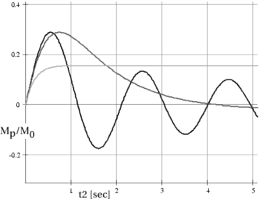
Figure 15.2: Plot of theoretical cross peak amplitude $M_{\perp p}^{I}$ vs. $t2$, for the case of negligible $T_{2}$ decay. $\beta=90^{\circ}$ and $\tau_{S}=200ms$. Three situations are shown:

Black - negligible diffusion

Dark Gray - diffusion of $M_{\parallel}$ has delayed the maximum and stretched the zero crossings to longer times.

Light Gray - $M_{\parallel}$ modulation has completely diffused away before the maximum can be obtained.

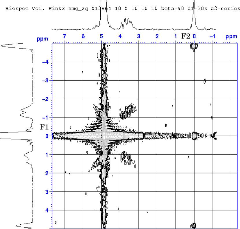
Figure 15.3: Representative low resolution 2d HOMOGENIZED spectrum. TSP is referenced to -4.7ppm on F1 axis and 0.0ppm on F2 Axis. Projections are restricted to [0, 4] ppm F2 and [-5, -1] ppm F1.

15.4 Experimental Results

A series of low resolution (512x64) HOMOGENIZED spectra were obtained with various strengths of $G_{zq}$ (see figure 15.3). The solvent (S) is water at room temperature, the solute of interest (I) was TSP at 100mM concentration. Glucose was also present in solution. Field strength is 4.7T yielding nominal $\tau_{S}=200ms$. A best fit, adjusting $M_{0}^{I}$and $\tau_{S}$ to account for pulse imperfections and $B_{1}$ inhomogeneity, was obtained for the top curve, and kept the same for the other curves. Relaxation rates were measured in separate inversion recovery and spin-echo experiments with $T_{1}^{S}=2.57s$, $T_{2}^{S}=140ms$ and $T_{2}^{I}=1.62s$. Effects such as $B_{1}$ inhomogeneity and RF pulse error contribute to lengthen $\tau_{Seff}$ (reduce available S magnetization). Comparison of the predicted cross peak amplitude with experiment is shown in figure 15.4.

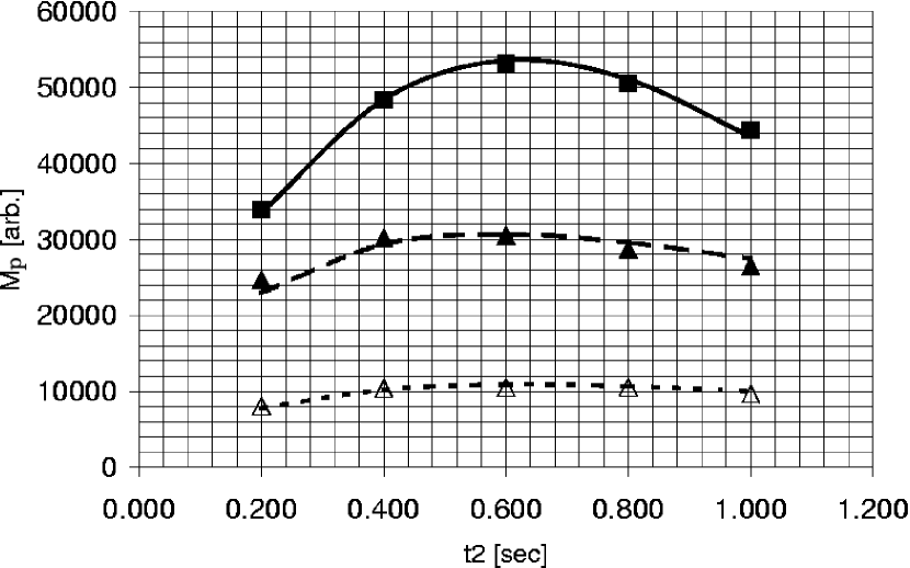
Figure 15.4: Data points and theoretical curve of p type TSP peak for three cases. Y axis arbitrary units.Data points and theoretical curve of p type TSP peak for three cases. Y axis arbitrary units.

$\alpha=\beta=90^{\circ}$, $\delta_{a}=\delta_{b}=\delta_{c}=1ms$, $\delta_{spoil}=5ms$

$G_{a}=G_{b}=G_{c}=G_{spoil}=20\frac{mT}{m}$, $\delta_{zq}=3ms$

Upper - $TR=20s,\,G_{zq}=10\frac{mT}{m}$

Middle - $TR=20s,\,G_{zq}=40\frac{mT}{m}$

Lower - $TR=2s,\,G_{zq}=40\frac{mT}{m}$

Chapter 16 SPATIALLY VARYING STEADY STATE LONGITUDINAL MAGNETIZATION

16.1 Introduction

NMR and MRI sequences utilizing the Distant Dipolar Field (DDF) have the relatively unique property of preparing, utilizing, and leaving spatially-modulated longitudinal magnetization, $M_{z}(s)$, where $\hat{s}$ is in the direction of an applied gradient. In fact this is fundamental to producing the novel “multiple spin-echo”[65, 68] or “non-linear stimulated echo” [127] of the classical picture and making the “intermolecular multiple quantum coherence (iMQC)” [71] observable in the quantum picture.

Existing analytical signal equations for DDF/iMQC sequences depend on $M_{z}(s)$ being sinusoidal during the signal build period[116, 75]. Experiments that probe sample structure also require a well-defined “correlation distance” which is defined as the repetition distance of $M_{z}(s)$ [76, 79, 128]. If the repetition time $TR$ of the DDF sequence is such that full relaxation is not allowed to proceed $TR<5T_{1}$, or diffusion does not average out the modulation, spatially-modulated longitudinal magnetization will be left at the end of one iteration of the sequence. The next repetition of the sequence will begin to establish “harmonics” in what is desired to be a purely sinusoidal modulation pattern. Eventually a steady state is established, potentially departing significantly from a pure sinusoid.

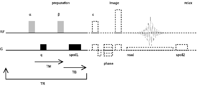
Figure 16.1: Pulse Sequence for measuring $M_{z}^{SS}(s)$. All RF pulses shown as hard for simplicity are actually Sinc3. $\alpha$ and $\beta$ are the same phase.

16.2 Experimental Methods

In order to study the behavior of the steady state $M_{z}^{SS}(s)$ profile we have implemented a looped DDF preparation subsequence followed by a standard multiple-phase encode imaging sub-sequence. (Figure 16.1.) The $\alpha$ pulse excites the system, the gradient $G_{q}$ twists the transverse magnetization into a helix. $\beta$ rotates one component of the helix back into the longitudinal direction. For simplicity we have omitted the $180^{\circ}$ pulses used to create a spin-echo during TM and/or TB sometimes present in DDF sequences. Also, we are only interested in $M_{z}(s)$ in this experiment, not the actual DDF-generated transverse signal. Looping the “preparation” sub-sequence thus creates the periodic $M_{z}(s)$ profile, spoils remaining transverse magnetization, and establishes $M_{z}^{SS}(s)$. The $\varepsilon$ pulse converts $M_{z}^{SS}(s)$ into transverse magnetization, allowing it to be imaged via the subsequent spin-echo “image” sub-sequence. $M_{z}^{SS}(s)$ must be re-established by the “preparation” sub-sequence for each phase encode. After a suitably long full relaxation delay “relax,” the sequence is repeated to acquire the next k-space line. This is clearly a slow acquisition method because many $TR$ periods are required to reach steady state in the preparation before each k-space line is acquired. The sequence is intended as a tool to directly image the $M_{z}^{SS}(s)$ profile, verifying the $M_{z}^{SS}(s)$ that would occur in a steady state DDF sequence, not as a new imaging modality.

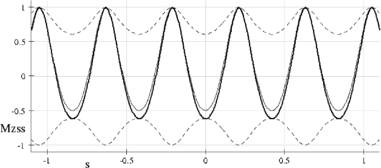
Figure 16.2: Theoretical values of $M_{z}(s)$. $M_{z}^{SS}(s)$is shown dashed $---$ as an envelope, $M_{z}^{SS,\,\beta}(s)$ is shown as a heavy line, $M_{z}^{SS,\,TB}(s)$ as a normal line. $\alpha=\beta=90^{\circ},\ TR=2s,\ TM=0ms,\ TB=100ms,\ \ T_{1}=1.4s$

16.3 Theory

The effect of the ”preparation” pulse sequence was first determined for a single iteration. The progress along the sequence is denoted by the the superscript.

Starting with fully relaxed equilibrium magnetization before the $\alpha$ pulse:

$$M_{z}^{Eq}(s)=M_{0}$$ (16.1)

after the $\alpha$ pulse, the mix delay $TM$ and the $\beta$ pulse we have:

$$M_{z}^{\beta}(s) =[A^{\beta}cos(q\,s)+B^{\beta}]\,M_{z}^{Eq}+C^{\beta}M_{0}$$ (16.2)

$$A^{\beta}=-sin(\alpha)\,e^{-\frac{TM}{T_{2}}}sin(\beta)$$

$$B^{\beta}=cos(\alpha)\,e^{-\frac{TM}{T_{1}}}cos(\beta)$$

$$C^{\beta}=(1-e^{-\frac{TM}{T_{1}}})\,cos(\beta)$$

The parameter $q=\frac{2\pi}{\lambda}$, where $\lambda$ is the helix pitch resulting from the applied gradient. Diffusion has been assumed to be negligible at the scale of $\lambda$. Note that $T_{2}$ is used in $A$ rather than $T_{2}^{*}$ when $G_{q}$ is larger than background inhomogeneity and susceptibility gradients.

After the build delay $TB$ we have:

$$M_{z}^{TB}(s)=[A^{TB}cos(q\,s)+B^{TB}]\,M_{z}^{Eq}(s)+C^{TB}M_{0}$$ (16.3)

$$A^{TB}=-sin(\alpha)\,e^{-\frac{TM}{T_{2}}}sin(\beta)\,e^{-\frac{TB}{T_{1}}}$$

$$B^{TB}=cos(\alpha)\,e^{-\frac{TM}{T_{1}}}cos(\beta)\,e^{-\frac{TB}{T_{1}}}$$

$$C^{TB}=[(1-e^{-\frac{TM}{T_{1}}})\,cos(\beta)-1]\,e^{-\frac{TB}{T_{1}}}+1$$

At the start of the next repetition, after a $TR$ period inclusive of $TM$ and $TB$ we have

$$M_{z}^{TR}(s)=[A^{TR}cos(q\,s)+B^{TR}]M_{z}^{Eq}(s)+C^{TR}\,M_{0}$$ (16.4)

$$A^{TR}=-sin(\alpha)\,e^{-\frac{TM}{T_{2}}}sin(\beta)\,e^{-\frac{TR-TM}{T_{1}}}$$

$$B^{TR}=cos(\alpha)\,cos(\beta)\,e^{-\frac{TR}{T_{1}}}$$

$$C^{TR}=[(1-e^{-\frac{TM}{T_{1}}})\,cos(\beta)-1]\,e^{-\frac{TR-TM}{T_{1}}}+1$$

If we apply the sequence $N$ times and re-arrange the terms we get the series:

$$M_{z}^{NxTR}(s)=M_{0}+M_{0\,}[A^{TR}cos(q\,s)+B^{TR}+C^{TR}-1]\sum\limits_{n=1}^{N}[A^{TR}cos(q\,s)+B^{TR}]^{n-1}$$ (16.5)

for the starting magnetization state after $N$ repetitions of the sequence.

Summing an infinite number of terms results in the expression for the steady state $M_{z}^{SS}(s)$ after a large number of TR periods:

$$M_{z}^{SS}(s)=M_{0}-M_{0\,}[\frac{A^{TR}cos(q\,s)+B^{TR}+C^{TR}-1}{A^{TR}cos(q\,s)+B^{TR}-1}]$$ (16.6)

One can then calculate the magnetization state after the $\beta$ pulse in the steady state:

$$M_{z}^{SS,\,\beta}(s)=[A^{\beta}cos(q\,s)+B^{\beta}]\,M_{z}^{SS}(s)+C^{\beta}M_{0}$$ (16.7)

and after $TB$:

$$M_{z}^{SS,\,TB}(s)=[A^{TB}cos(q\,s)+B^{TB}]\,M_{z}^{SS}(s)+C^{TB}M_{0}$$ (16.8)

We show graphs of equations [16.6], [16.7], and [16.8] in Figure 16.2 for $TR=2s$.

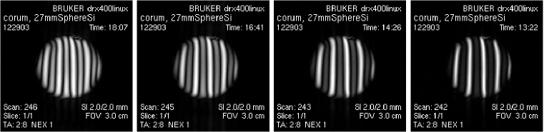
Figure 16.3: $M_{z}^{SS}(s)$ images, $TR=5s,\ 2s,\ 1s,\ 500ms$ from left to right. $TM=TB=\leavevmode\nobreak\ 7ms,\ relax=10s$.

16.4 Results

We now show in Figure 16.3 representative $M_{z}^{SS}(s)$ magnitude images obtained with the sequence described in section 16.2 for four different values of $TR=5s,\ 2s,\ 1s,\ 500ms$. Figure 16.4 shows several cross sections through row #128 of Figure 16.3. The object is an 18mm glass sphere filled with silicone oil. Data points are superimposed with the corresponding magnitude of the theoretical curve. The $T_{1}$ of the silicone oil (at 400MHz) was measured by spectroscopic inversion recovery to be 1.4s. A Bruker DRX400 Micro 2.5 system was used with a custom 27mm diameter 31P/1H birdcage coil. 10 $TR$ periods were used to establish steady state. A 10s “relax” delay was used between phase encodes to establish full relaxation. $G_{q}$ was 3ms and 2.5mT/mm, with $G_{spoil1}$ of 5ms and 100mT/mm. No attempt was made to account for $B_{1}$ inhomogeneity. A single scaling parameter was used for all theoretical curves. We achieved good agreement with the theoretical predictions. In the sequence as used, $TM=TB=\leavevmode\nobreak\ 7ms$. A variety of other $G_{q}$ directions and strengths show similar agreement with theory. Better agreement in the fit between experiment and theory can be obtained with $\alpha=\beta=75^{\circ}$than with the nominal $90^{\circ}$. A $B_{1}$ map needs to be determined to see if this corresponds more closely to the actual experimental conditions.

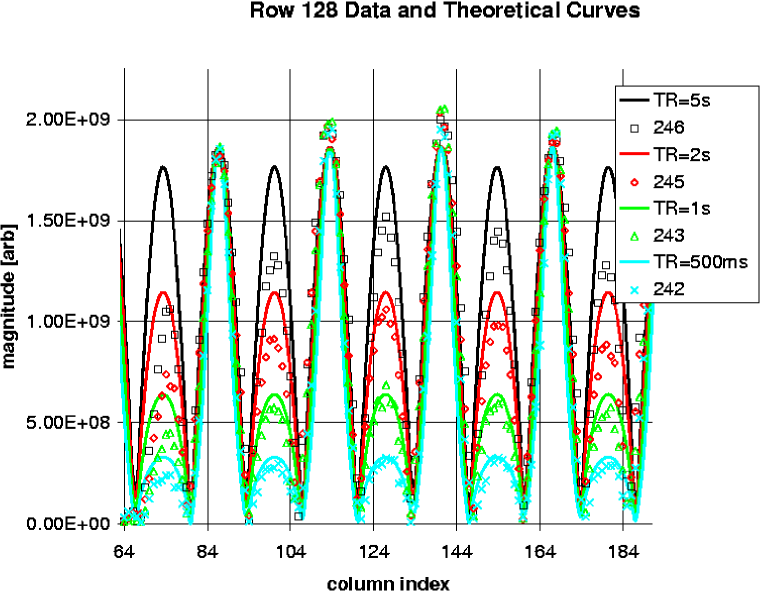
Figure 16.4: Comparison of theory and experiment for steady state $M_{Z}$. Row 128 data (points) and Fit (lines), $\alpha=\beta=90^{\circ},\ TR=2s,\ TM=TB=7ms,\ \ T_{1}=1.4s\ relax=10s$.

16.5 Conclusions

The expressions developed and verified above should be useful to those wishing to understand or utilize harmonics in the $M_{z}^{SS}(s)$ profile in DDF based sequences in the situation where the diffusion distance during $TR$ compared with $\lambda$ in negligible. This is especially true for those carrying out structural measurements which depend on a well defined correlation distance. The theory should also hold for spatially-varying magnetization density $M_{0}=M_{0}(\vec{r})$, and longitudinal relaxation $T_{1}=T_{1}(\vec{r})$.

Chapter 17 THE FUTURE OF DDF NMR AND HOMOGENIZED

Research into DDF effects has only been ongoing for just over a decade. There is still much more to be learned about the DDF and DDF based applications in MRI and MRS. We can identify several fruitful lines of research that still need more investigation.

There is still a lot to be learned about the imaging properties of DDF based sequences, such as the point spread function, contrast mechanisms, and whether the signal is truly “local” to a voxel. There have been a number of interesting imaging applications, beyond the initial work of try it and see what it looks like. A very intriguing application is “Multiple-Quantum Vector Imaging” which is a fancy term for utilization of the gradient direction to detect the orientation of sub-voxel structures [84].

Much work has been done on using the DDF to image porous structures, and in-vivo there has been much interest in quantifying trabecular bone density[129, 77, 128, 81, 98, 82]. This work continues.

The author’s (as well as at least one other research group’s) work has recently focused on adding localization to HOMOGENIZED in order to get spectra from a voxel in-vivo. There have been some initial successes [130, 131]. The signal equations developed in this dissertation, and extensions, should be useful for quantification of metabolites utilizing these new localized HOMOGENIZED sequences.

There have been recent improvements [89, 88] to HOMOGENIZED, utilizing selective pulses on the solvent $S$ to suppress water and boost crosspeak signal.

Quantification of HOMOGENIZED peaks (in vitro and in vivo) is still an active and needed research topic. Continuing the author’s work and the work of Ardelean [74] should help quantify the effects of $T_{1}$ relaxation during the $\tau_{mix}$ and $\tau_{echo}$ time periods of HOMOGENIZED.

Related to the issue of quantification is determining HOMOGENIZED’s sensitivity to pulse errors, which is magnified by DDF refocusing. Using HOMOGENIZED with adiabatic pulses should help reduce this issue, and has recently been demonstrated [130].

HOMOGENIZED based Spectroscopic Imaging is an intriguing possibility. It would have many advantages, such as its self referencing properties which eliminate the need for frequency shift correction (and phasing).

Part III APPENDICES

Appendix A SOME DERIVATIONS

A.1 Equilibrium Magnetization

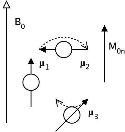
Figure A.1: Individual Nuclear Magnetic Moments in a Magnetic Field

Any sample in an NMR experiment is composed of a large number of identical nuclei loosely coupled to each other and the external environment (FigureA.1.) The dominant coupling is to an external applied magnetic field $\vec{B_{0}}$. Each nucleus possesses magnetic potential energy

$$E_{n}=-\vec{\mu}_{n}\cdot\vec{B}_{0}.$$ (A.1)

The field will tend to cause the moments of the nuclei to align parallel to the field, minimizing the total magnetic energy

$$E=-\sum_{N}\vec{\mu}_{n}\cdot\vec{B}_{0}.$$ (A.2)

In competition with the field, thermal excitation will tend to randomize the alignment.

The net macroscopic magnetic moment per unit volume is defined as

$$\vec{M}\equiv\frac{1}{V}\sum_{N}\vec{\mu}_{n}.$$ (A.3)

Since there is coupling to the environment, the sample/environment system will eventually come to thermal equilibrium. The equilibrium magnetization can be found by the Boltzmann law of statistical mechanics[36, Ch I, A. p. 2] $P(E_{m})\propto e^{-E_{m}/k\,T}$ where $P(E_{m})$ is the probability of finding a nuclear moment in energy state $E_{m}$, $T$ is the absolute temperature, and $k=1.3806505\times 10^{-23}[\frac{J}{K}]$ [132] is the Boltzmann constant. The number of energy levels is determined by the total spin quantum number $I$ and “z” component $m$ with $I\geq m\geq-I$ with $\Delta m=1$. We have

$$\vec{<M>_{eq}}=\frac{1}{V}\sum_{N}[\sum_{m=-I}^{I}\vec{\mu_{n}}P(E_{n})\,/\sum_{m=-I}^{I}P(E_{n})].$$ (A.4)

Assuming that the field $B_{0}$ is oriented in the $\hat{z}$ direction, only the $\hat{z}$ component of $\vec{\mu}$ effects the energy, and all orthogonal directions of $\vec{\mu}$ are equally probable, averaging to zero. The $z$ component quantum number $m$ then determines the potential energy, and $\vec{<M>_{eq}}=M_{0}\hat{z}$ is oriented along the $z$ axis. We also make the substitution $\mu=\left|\vec{\mu}\right|$=$\gamma\hbar I$ where $\gamma$ is the magnetogyric ratio. Since $N$ is a very large number we are in effect taking an ergodic average. We can assume that $M_{0}$ does not fluctuate, and drop the expectation brackets to get

$$M_{0}=\frac{\mu}{V}\sum_{N}[\sum_{m=-I}^{I}m\,e^{\frac{m\,\gamma\,\hbar\,B_{0}}{k\,T}}/\sum_{m=-I}^{I}e^{\frac{m\,\gamma\,\hbar\,B_{0}}{k\,T}}].$$ (A.5)

Applying the so-called high temperature approximation

$$k\,T\gg\gamma\,\hbar\,B_{0},$$ (A.6)

valid for nearly all but ultra-cold temperature and ultrahigh fields, yields

$$e^{\frac{m\,\gamma\,\hbar\,B_{0}}{k\,T}}\approx 1+\frac{m\,\gamma\,\hbar\,B_{0}}{k\,T}.$$ (A.7)

Substituting, we get

$$M_{0}\approx\frac{\gamma\,\hbar}{V}\sum_{N}[\sum_{m=-I}^{I}m+\frac{m^{2}\gamma\,\hbar\,B_{0}}{k\,T}/\sum_{m=-I}^{I}1+\frac{m\,\gamma\,\hbar\,B_{0}}{k\,T}].$$ (A.8)

Carrying out the summation operations gives

$$M_{0}\approx\frac{\gamma^{2}\hbar^{2}N\,B_{0}I\,(I+1)}{3\,V\,k\,T}.$$ (A.9)

Note since $\frac{\hbar\,B_{0}}{k\,T}\ll 1$, $\vec{<M>_{eq}}\ll\frac{N\,\gamma\,\hbar\,I}{V}$, is much less than the theoretical maximum achievable magnetization (saturation magnetization) at low temperature or ultrahigh field. For ${}^{1}H$ water $\frac{N}{V}=2[protons]\times 55.56\times 10^{-3}[mol\,cm^{-3}]\times N_{A}[mol^{-1}]=6.6918\times 10^{22}[protons\,cm^{-3}]$, $\gamma_{p}=2.675\times 10^{8}$ at $T=310\,K$ (body temperature) and $B_{0}=3\,T$ the ratio $\frac{M_{0}}{M_{sat}}=9.89\times 10^{-6}$$\approx 10^{-5}$ a very small fraction.

We can also use the above to define the nuclear magnetic susceptibility $\chi$. From the relation

$$M_{0}=\frac{\chi}{\mu_{0}}B_{0},$$

we get

$$\chi=\frac{\mu_{0}\gamma^{2}\hbar^{2}N\,I\,(I+1)}{3\,V\,k\,T},$$

where $\mu_{0}=4\pi\times 10^{-7}\frac{N}{A^{2}}$is the permeability of free space. A quick check will show that $\chi$ is indeed dimensionless.

A.2 Cross Product with $M_{\parallel}$ and $M_{\perp}$

Of most interest for the Bloch equations is the cross product of $\vec{M}\times\vec{B}$ in terms longitudinal and transverse components. In Cartesian coordinates the cross product is defined as

$$\vec{M}\times\vec{B}=\left|\begin{array}[]{ccc}M_{x}&M_{y}&M_{z}\\ B_{x}&B_{y}&B_{z}\\ \hat{x}&\hat{y}&\hat{z}\end{array}\right|=(M_{y}B_{z}-M_{z}B_{y})\,\hat{x}-(M_{x}B_{z}-M_{z}B_{x})\,\hat{y}+(M_{x}B_{y}-M_{y}B_{x})\,\hat{z}.$$ (A.10)

In the complex representation we have

$$\begin{array}[]{cc}M_{\parallel}=M_{z}&\;B_{\parallel}=B_{z}\end{array}$$ (A.11)

and

$$\begin{array}[]{cc}M_{\perp}=M_{x}+i\,M_{y}&\;B_{\perp}=B_{x}\end{array}+i\,B_{y}.$$ (A.12)

We note that the longitudinal and transverse components of the cross product are

$$[\vec{M}\times\vec{B}]_{\parallel}=M_{x}B_{y}-M_{y}B_{x}$$ (A.13)

and

$$[\vec{M}\times\vec{B}]_{\perp}=(M_{y}B_{z}-M_{z}B_{y})-i\,(M_{x}B_{z}-M_{z}B_{x}).$$ (A.14)

By substituting

$$\begin{array}[]{cc}M_{x}=\frac{1}{2}(M_{\perp}+M_{\perp}^{*})&M_{y}=\frac{i}{2}(M_{\perp}-M_{\perp}^{*})\end{array},$$ (A.15)

and similarly for $B_{x}$and $B_{y}$ we find

$$[\vec{M}\times\vec{B}]_{\parallel}=\frac{i}{2}(M_{\perp}B_{\perp}^{*}-M_{\perp}^{*}B_{\perp})$$ (A.16)

and

$$[\vec{M}\times\vec{B}]_{\perp}=i\,(M_{\parallel}B_{\perp}-M_{\perp}B_{\parallel}).$$ (A.17)

A.3 Fourier Transform of $\frac{\Lambda(\vec{r})}{r^{3}}$

This is a derivation of fundamental importance to distant dipolar field theory and calculation. The result in the form used was first published in Deville et al. 1979 [65] who references Leggett [133, Appendix II] for the derivation. The derivation in Leggett is somewhat terse, so we carry it out here in detail with some variation and much enhancement for completeness.

Starting with the general form of the transform

$$\mathcal{F}_{3}\{\frac{\Lambda(\vec{r})}{r^{3}}\}\equiv\int_{\infty}d^{3}r\,e^{-i\,2\pi\,\vec{\rho}\cdot\vec{r}}\frac{\Lambda(\vec{r})}{r^{3}},$$ (A.18)

we put it into spherical polar coordinates

$$\mathcal{F}_{3}\{\frac{\Lambda(\vec{r})}{r^{3}}\}=\int_{0}^{2\pi}d\phi\,\int_{0}^{\pi}d\theta\,sin(\theta)\,\int_{0}^{\infty}dr\,r^{2}e^{-i\,2\pi\,\vec{\rho}\cdot\vec{r}}\frac{\Lambda(\vec{r})}{r^{3}}.$$ (A.19)

We then constrain $\vec{\rho}=\rho\,\hat{z}$ and simplify to get

$$\mathcal{F}_{3}\{\frac{\Lambda(\vec{r})}{r^{3}}\}=\int_{0}^{2\pi}d\phi\,\int_{0}^{\pi}d\theta\,sin(\theta)\,\int_{0}^{\infty}\frac{dr}{r}\,e^{-i\,2\pi\,\rho\,r\,cos(\theta)}\Lambda(\vec{r}).$$ (A.20)

We note that $\Lambda(\vec{r})=P_{2}[cos(\theta)]$ where $P_{n}$ is the $n$th Legendre polynomial. We now recognize the integral representation of the Spherical Bessel function [134, 10.1.14, p. 438] of order $n$ with $z=-2\pi\,r\,\rho$ and $n=2$, which is

$$j_{n}(z)=\frac{(-i)^{n}}{2}\int_{0}^{\pi}d\theta\,sin(\theta)\,e^{i\,z\,cos(\theta)}P_{n}[cos(\theta)].$$ (A.21)

Substitution leaves us with

$$\mathcal{F}_{3}\{\frac{\Lambda(\vec{r})}{r^{3}}\}=-2\int_{0}^{2\pi}d\phi\,\int_{0}^{\infty}\frac{dr}{r}\,j_{2}(-2\pi\,r\,\rho),$$ (A.22)

where $j_{n}$ can be generated from [134, 10.1.25, p. 439]

$$j_{n}(z)=z^{n}(-\frac{1}{z}\frac{\partial}{\partial z})^{n}[\frac{sin(z)}{z}].$$ (A.23)

The first few spherical Bessel functions are

$$j_{0}(z)=\frac{sin(z)}{z},$$ (A.24)

$$j_{1}(z)=-\frac{cos(z)}{z}+\frac{sin(z)}{z^{2}}$$ (A.25)

and

$$j_{2}(z)=-3\frac{cos(z)}{z^{2}}+\frac{(3-z^{2})\,sin(z)}{z^{3}}.$$ (A.26)

We can evaluate the integral by integrating both sides of the recurrence relations [134, 10.1.21-22, p. 439] obtaining the identity

$$\int_{0}^{\infty}dz\,\frac{j_{n}(z)}{z}=\frac{n-2}{n+1}\int_{0}^{\infty}dz\,\frac{j_{n-2}(z)}{z}-\frac{1}{n+1}[j_{n-2}(z)-j_{n}(z)]_{0}^{\infty}.$$ (A.27)

Specifically we have

$$\int_{0}^{\infty}dz\,\frac{j_{2}(z)}{z}=\frac{0}{3}\int_{0}^{\infty}dz\,\frac{j_{0}(z)}{z}-\frac{1}{3}[j_{0}(z)-j_{2}(z)]_{0}^{\infty}=\frac{1}{3},$$ (A.28)

leading to

$$\mathcal{F}_{3}\{\frac{\Lambda(\vec{r})}{r^{3}}\}=-\frac{4\pi}{3},$$ (A.29)

and remembering the condition

$$\vec{\rho}=\rho\,\hat{z}.$$ (A.30)

For the case of general $\vec{\rho}$ it is easier to consider rotation of the function being transformed, leaving $\vec{\rho}=\rho\,\hat{z}$. We consider rotation of $\Lambda(\vec{r})$ around an arbitrary pair of angles $\theta_{0}$ and $\phi_{0}$ leading to

$$\Lambda_{rot}(\vec{r})=P_{2}[cos(\alpha)],$$ (A.31)

with

$$cos(\alpha)=cos(\theta)\,cos(\theta_{0})+sin(\theta)\,sin(\theta_{0})\,cos(\phi-\phi_{0}).$$ (A.32)

We need only consider $\theta_{0}$ and can set $\phi_{0}=0$ without loss of generality due to the azimuthal symmetry of $\Lambda(\vec{r})$.

We use the spherical harmonic addition theorem [117, 8.794 1., p. 1013], [135, eq. (5.83), p. 257 ]

$$P_{l}[cos(\alpha)]=\frac{4\pi}{2l+1}\sum_{m=-l}^{l}Y_{l\,m}^{*}(\theta_{0},\,\phi_{0})\,Y_{l,\,m}(\theta,\,\phi)$$ (A.33)

where the spherical harmonics are defined [135, eq. (5.75), p. 255] as

$$Y_{l\,m}(\theta,\,\phi)\equiv(-1)^{m}\left[\frac{2l+1}{4\pi}\frac{(l-m)!}{(l+m)!}\right]^{1/2}P_{l}^{m}[cos(\theta)]\,e^{i\,m\,\phi}$$ (A.34)

with the condition

$$m\geq 0$$ (A.35)

and further definition

$$Y_{l,\,-m}(\theta,\,\phi)\equiv(-1)^{m}Y_{l\,m}^{*}(\theta,\,\phi).$$ (A.36)

After substitution of $l=2$ and $\phi_{0}=0$ and application of the above definition we have

$$P_{2}[cos(\alpha)]=\frac{4\pi}{5}\{Y_{2,\,2}(\theta_{0},\,0)\,[Y_{2,\,2}(\theta,\,\phi)-Y_{2,\,2}^{*}(\theta,\,\phi)]\\ +Y_{2,\,1}(\theta_{0},\,0)\,[Y_{2,\,1}(\theta,\,\phi)-Y_{2,\,1}^{*}(\theta,\,\phi)]+Y_{2,\,0}(\theta_{0},\,0)\,Y_{2,\,0}(\theta,\,\phi)\}.$$ (A.37)

We note that the $\phi$ dependence of the spherical harmonic term is

$$Y_{l,\,m}(\theta,\,\phi)-Y_{l,\,m}^{*}(\theta,\,\phi)\sim cos(m\,\phi)$$ (A.38)

and that when evaluated in the $\phi$ integral we have

$$\int_{0}^{2\pi}cos(m\,\phi)\,d\phi=[_{0}^{2\pi}\frac{sin(m\,\phi)}{m}=0$$ (A.39)

for integer $m\neq 0$. The only term that survives the $\phi$ integration is the $\phi$ independent part

$$\frac{4\pi}{5}Y_{2,\,0}(\theta_{0},\,0)\,Y_{2,\,0}(\theta,\,\phi)=P_{2}[cos(\theta_{0})]\,P_{2}[cos(\theta)],$$ (A.40)

leading to the result

$$\mathcal{F}_{3}\{\frac{\Lambda_{rot}(\vec{r})}{r^{3}}\}=-\frac{4\pi}{3}P_{2}[cos(\theta_{0})].$$ (A.41)

Considering the rotation of $\vec{\rho}$ instead of $\Lambda$ we have our desired result

$$\mathcal{F}_{3}\{\frac{\Lambda(\vec{r})}{r^{3}}\}=-\frac{4\pi}{3}\Lambda(\vec{\rho}).$$ (A.42)

A.4 Secular Component of the Field of a Point Dipole

We start with the magnetic field of an arbitrarily oriented point dipole $\vec{\mu}$,

$$\vec{B}_{dip}=\frac{\mu_{0}}{4\pi}\frac{3\,(\vec{\mu}\cdot\hat{r})\,\hat{r}-\vec{\mu}}{r^{3}}.$$ (A.43)

The secular component is the component that is invariant to rotation of the coordinate axes about $\vec{B}_{0}=B_{0}\hat{z}$. This definition at first appears to suggest that the secular component is just the $\hat{z}$ component of $\vec{B}_{dip}$. This is not so. While it does include the $\hat{z}$ component, it can also include non $\hat{z}$ components as well. The operative definition is

$$\vec{B}_{secular}=\frac{1}{2\pi}\int_{0}^{2\pi}\vec{B}_{dip}d\phi.$$ (A.44)

Consider $\vec{\mu}$ with arbitrary orientation

$$\vec{\mu}=\mu\,[cos(\theta_{\mu})\,\hat{z}+sin(\theta_{\mu})\,cos(\phi_{\mu})\,\hat{x}+sin(\theta_{\mu})\,sin(\phi_{\mu})\,\hat{y}]$$ (A.45)

and the definition of $\hat{r}$

$$\hat{r}\equiv cos(\theta)\,\hat{z}+sin(\theta)\,cos(\phi)\,\hat{x}+sin(\theta)\,sin(\phi)\,\hat{y}.$$ (A.46)

We substitute into our expression for $\vec{B}_{dip}$ and split into Cartesian components

$$B_{x}=\frac{\mu_{0}}{4\pi}\frac{\mu}{r^{3}}[3\,sin(\theta)\,cos(\theta)\,cos(\phi)\,cos(\theta_{\mu})-sin(\theta_{\mu})\,cos(\phi_{\mu})\\ +3\,sin^{2}(\theta)\,cos^{2}(\phi)\,sin(\theta_{\mu})\,cos(\phi_{\mu})+3\,sin^{2}(\theta)\,sin(\phi)\,cos(\phi)\,sin(\theta_{\mu})\,sin(\phi_{\mu})]$$ (A.47)

$$B_{y}=\frac{\mu_{0}}{4\pi}\frac{\mu}{r^{3}}[3\,sin(\theta)\,cos(\theta)\,sin(\phi)\,cos(\theta_{\mu})-sin(\theta_{\mu})\,sin(\phi_{\mu})\\ +3\,sin^{2}(\theta)\,sin(\phi)\,cos(\phi)\,sin(\theta_{\mu})\,cos(\phi_{\mu})+3\,sin^{2}(\theta)\,sin^{2}(\phi)\,sin(\theta_{\mu})\,sin(\phi_{\mu})]$$ (A.48)

$$B_{z}=\frac{\mu_{0}}{4\pi}\frac{\mu}{r^{3}}\{[3\,cos^{2}(\theta)-1]\,cos(\theta_{\mu})\\ +3\,sin(\theta)\,cos(\theta)\,cos(\phi)\,sin(\theta_{\mu})\,cos(\phi_{\mu})+3sin(\theta)\,cos(\theta)\,sin(\phi)\,sin(\theta_{\mu})\,sin(\phi_{\mu})\}$$ (A.49)

We now perform the integral A.44, by Cartesian components, yielding

$$B_{x,\,secular}=\frac{1}{2\pi}\int_{0}^{2\pi}B_{x}d\phi=\frac{\mu_{0}}{4\pi}\frac{\mu}{r^{3}}[-sin(\theta_{\mu})\,cos(\phi_{\mu})+\frac{3}{2}\,sin^{2}(\theta)\,sin(\theta_{\mu})\,cos(\phi_{\mu})],$$ (A.50)

$$B_{y,\,secular}=\frac{1}{2\pi}\int_{0}^{2\pi}B_{y}d\phi=\frac{\mu_{0}}{4\pi}\frac{\mu}{r^{3}}[-sin(\theta_{\mu})\,sin(\phi_{\mu})+\frac{3}{2}\,sin^{2}(\theta)\,sin(\theta_{\mu})\,sin(\phi_{\mu})],$$ (A.51)

and

$$B_{z,\,secular}=\frac{1}{2\pi}\int_{0}^{2\pi}B_{z}d\phi=\frac{\mu_{0}}{4\pi}\frac{\mu}{r^{3}}[3\,cos^{2}(\theta)-1]\,cos(\theta_{\mu}).$$ (A.52)

Performing the substitution $sin^{2}(\theta)\equiv 1-cos^{2}(\theta)$ gives us

$$B_{x,\,secular}=-\frac{\mu_{0}}{4\pi}\frac{\mu}{r^{3}}[\frac{3\,cos^{2}(\theta)-1}{2}]\,sin(\theta_{\mu})\,cos(\phi_{\mu}),$$ (A.53)

$$B_{y,\,secular}=-\frac{\mu_{0}}{4\pi}\frac{\mu}{r^{3}}[\frac{3\,cos^{2}(\theta)-1}{2}]\,sin(\theta_{\mu})\,sin(\phi_{\mu}).$$ (A.54)

We note

$$B_{z,\,secular}=-(1-3)\frac{\mu_{0}}{4\pi}\frac{\mu}{r^{3}}[\frac{3\,cos^{2}(\theta)-1}{2}]\,cos(\theta_{\mu}).$$ (A.55)

Finally, we assemble the components into vector form as

$$\vec{B}_{secular}=\frac{\mu_{0}}{4\pi}\frac{1}{r^{3}}[\frac{3\,cos^{2}(\theta)-1}{2}]\,(3\,\mu_{z}\hat{z}-\vec{\mu}).$$ (A.56)

Appendix B The Levitt Sign Conventions

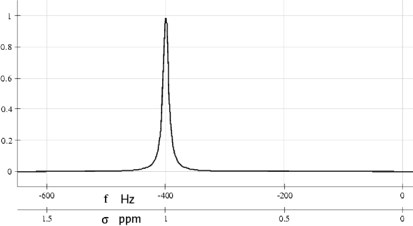
Figure B.1: Single peak at 1 ppm by the Levitt sign convention (on a $400\,MHz$ spectrometer). Note that the Levitt sign convention correctly accounts for increasing chemical shift toward the right, for Nuclei with positive $\gamma$ and hence negative Larmor frequency.

We briefly review the sign conventions presented in references [15, 9, section 2.5] which are followed throughout this dissertation. The convention properly accounts for the sense of rotation of net macroscopic magnetization. First we have

$$\omega_{0}\equiv-\gamma\,B_{0}$$

and

$$f_{0}\equiv\frac{\omega_{0}}{2\,\pi}$$

which leads to $negative$ Larmor frequency $f_{0}$ when $\gamma>0$. Negative Larmor frequency corresponds to left handed precession about the $B_{0}$ field. We define the chemical shift (in units of parts-per-million or $ppm$) as

$$\delta-\delta_{ref}\equiv 10^{6}\frac{\omega_{0}-\omega_{ref}}{\omega_{ref}},$$

where $\omega_{ref}$ is the angular Larmor frequency of a reference compound, such as $TMS$ or $DMS$ in high resolution NMR. These compounds are often defined as $\delta_{ref}=0\,ppm$. For in-vivo spectroscopy water is often the reference and is defined as $\delta_{ref}=4.7\,ppm$. Note that the Levitt sign convention also properly accounts for the “inverted” axis in NMR spectroscopy where increasing $positive$ chemical shift is plotted toward the left, since it corresponds to increasing $negative$ difference in Larmor frequency.

Appendix C Physical Constants

From [132].

symbol	name	value (uncertainty) [units]
$\gamma_{p}$	Proton Magnetogyric Ratio	$-2.675\,222\,05(23)\times*10^{8}[s^{-1}T^{-1}]$
$\frac{\gamma_{p}}{2\pi}$		-$42.577\,481\,3(37)\,[MHz\,T^{-1}]$
$h$	Planck Constant	$6.626\,069\,3(11)\times 10^{-34}[J\,s]$
$\hbar$	hbar, $\frac{h}{2\pi}$	$1.054\,571\,68(18)\times 10^{-34}[J\,s]$
$k$	Boltzmann Constant	$1.380\,650\,5(24)\times 10^{-23}[J\,K^{-1}]$
$\mu_{0}$	permeability of free space	$4\pi\times 10^{-7}[N\,A^{-2}]$
$\mu_{p}$	Proton Magnetic Moment	$1.420\,606\,71(12)\times 10^{-26}[J\,T^{-1}]$
$N_{A}$	Avogadro Constant	$6.022\,141\,5(10)\times 10^{23}[mol^{-1}]$
$\pi$	Pi, circle ratio	$3.141\,592\,653\,589\,793\,238$

Table C.1: Physical Constants

Appendix D NMR Data

atom	% abundance	Spin	$\gamma\ 10^{7}[\frac{rad}{T\,s}]$	Q	f[MHz]@11.744T	rel. sens.	abs. sens.
${}^{1}H$	$99.980$	$\frac{1}{2}$	$+26.7519$	$0$	$-500.000$	$1.00$	$1.00$
${}^{2}H$	$1.5\times 10^{-2}$	$1$	$+4.1066$	$2.8\times 10^{-3}$	$-76.753$	$6.65\times 10^{-6}$	$1.45\times 10^{-6}$
${}^{13}C$	$1.108$	$\frac{1}{2}$	+$6.7283$	$0$	$-125.721$	$1.59\times 10^{-2}$	$1.76\times 10^{-4}$
${}^{15}N$	$.365$	$\frac{1}{2}$	$-2.7120$	$0$	$+50.664$	$1.04\times 10^{-3}$	$3.85\times 10^{-6}$
${}^{19}F$	$100.000$	$\frac{1}{2}$	+$25.181$	$0$	$-470.385$	$.83$	$.83$
${}^{31}P$	$100.000$	$\frac{1}{2}$	+$10.841$	$0$	$-202.404$	$6.63\times 10^{-2}$	$6.63\times 10^{-2}$
${}^{129}Xe$	$26.44$	$\frac{1}{2}$	$-7.452$	$0$	$+139.045$	$2.12\times 10^{-2}$	$5.6\times 10^{-3}$

from [136, 9]

Table D.1: Some common Nuclei in NMR

Index

• 180 degree pulse §3.2.2
• 90 degree pulse §3.2.1
• adiabatic pulse §3.1
• b-value §10.1.4
• B0 inhomogeneity §4.3
• B1 inhomogeneity §3.1
• bandwidth (of and RF pulse) §3.3
• Bessel function §14.4, §14.5
• Bloch, Felix §1.2
• Bowtell, R. §11.1
• Carr-Purcell-Meiboom-Gill Chapter 5
• correlation distance §11.4, §15.2.3, §16.1
• CPMG Chapter 5
• cross-product §A.2
• crushing Chapter 6
• DDF §1.1, Chapter 11, §11.1, §11.4, §12.1, §12.2, §12.3, §14.3, §14.3.5, §14.4, §15.1, §15.2.5, §15.3, Chapter 17
• DDF as an effective gradient §12.2
• Deville §11.4, §11.6
• diffusion Chapter 5, Chapter 7
• diffusion weighted §10.1.9, §7.2.1
• diffusion weighting §15.2.2, §7.2.1
• dipolar demagnetization time §12.2
• dipolar demagnetizing field §11.1, §11.3
• distant dipolar field §1.1, Chapter 11, §11.1
• echo-time Chapter 5
• egodic average §7.1.1
• Ernst angle §14.3.1, §4.1.1
• excitation pulse §3.2.1
• FID §3.4
• field inhomogeneity §4.3
• Free Induction Decay §3.4
• Free Induction Decay, FID Chapter 5
• gradients Chapter 6
• gyromagnetic ratio §2.3
• Hahn, E. L. Chapter 5
• HOMOGENIZED §1.1, §11.1, §14.1
• imaging §16.2
• iMQC §11.1, §16.1
• in-vivo magnetic resonance spectroscopy §11.1
• in-vivo spectroscopy §15.1
• intermolecular multiple quantum coherence §11.1
• intermolecular zero quantum coherencecoherence §15.1
• inversion pulse §3.2.2
• iZQC §15.1
• Korber, H. §11.1
• Larmor frequency §2.3, §6.2
• Legendre polynomial §A.3
• local form §11.4
• longitudinal magnetization Chapter 16
• longitudinal relaxation §4.1
• macroscale §11.1
• magic angle §11.2
• magnetic dipole §11.2
• magnetic resonance imaging §1.1
• magnetic resonance spectroscopy §1.1
• magnetic susceptibility §2.2
• magnetogyric ratio §2.3
• mesoscale §11.1
• microscale §11.1
• motional narrowing Chapter 7
• MRI §1.1, §16.1, Chapter 17
• MRS §1.1, §11.1, §15.1, Chapter 17
• multiple quantum vector imaging Chapter 17
• NMR §11.1, §16.1
• nmr diffraction §11.5
• nmr spectrum §3.4.2
• Nobel Prize §1.2
• non-linear bloch equations Chapter 12
• point form §11.6
• Precession §2.3
• pulse sequence §6.1.1
• pulsed-gradient spin-echo §10.1
• Purcell, Edward §1.2
• quadrature detection §3.4.1
• Rabi, I. I. §1.2
• radiation damping Chapter 13, §15.2.2
• random walk Chapter 7
• reciever coil §3.4
• recovery (of longitudinal magnetization) §4.1.1
• relaxation Chapter 4
• repetition time §4.1.1
• RF field §3.1
• RF pulse §3.2
• sample inhomogeneity §4.3
• Secular Approximation §6.2
• secular component §11.2
• self-diffusion §7.2
• slowly varying §11.6
• spatially-dependent modulation §12.1
• spectroscopic maging Chapter 17
• spectrum §3.4.2
• sphere of Lorentz §11.4
• Spherical Bessel function §A.3
• spin-echo §14.3.5, Chapter 5
• spin-lattice relaxation §4.1
• spin-spin relaxation §4.2
• spoiling Chapter 6
• spontaneous emission §4.1
• Stejskal-Tanner §15.2.2
• susceptibility gradients §4.3
• T1 §4.1
• T2 §4.2
• T2 dagger §4.3
• T2 star §4.3
• TE Chapter 5
• TR §4.1.1
• transmit coil §3.1
• transverse magnetization §6.1
• transverse relaxation §4.2
• Warren, W. §11.1

References

- [1] S. Kennedy, B. Razavi, Z. Chen, and J. Zhong, “Diffusion Measurements Free of Motion Artifacts Using Intermolecular Dipole-Dipole Interactions,” in ISMRM Proceedings, vol. 11, International Society for Magnetic Resonance in Medicine, July 2003. talk 0581.
- [2] S. Vathyam, S. Lee, and W. Warren, “Homogeneous NMR Spectra in Inhomogeneous Fields,” Science, vol. 272, pp. 92–96, 5 Apr. 1996.
- [3] R. J. Gillies, J. P. Galons, K. A. McGovern, P. G. Scherer, Y. H. Lien, C. Job, R. Ratcliff, F. Chapa, S. Cerdan, and B. E. Dale, “Design and Application of NMR-Compatible Bioreactor Circuits for Extended Perfusion of High-Density Mammalian-Cell Cultures,” NMR In Biomedicine, vol. 6, pp. 95–104, Jan. 1993.
- [4] I. I. Rabi, J. R. Zacharias, S. Millman, and P. Kusch, “A New Method of Measuring Nuclear Magnetic Moment,” Phys. Rev., vol. 53, p. 318, 15 Feb. 1938.
- [5] I. I. Rabi, S. Millman, P. Kusch, and J. R. Zacharias, “The Molecular Beam Resonance Method for Measuring Nuclear Magnetic Moments The Magnetic Moments of 3Li6, 3Li7 and 9F19,” Phys. Rev., vol. 55, pp. 526–535, 15 Mar. 1938.
- [6] E. Purcell, H. Torrey, and R. Pound, “Resonance Absorption by Nuclear Magnetic Moments in a Solid,” Physical Review, vol. 69, pp. 37–38, 1 Jan. 1946.
- [7] F. Bloch, W. Hansen, and M. Packard, “The Nuclear Induction Experiment,” vol. 70, pp. 474–485, 1 Oct. 1946.
- [8] H. Pfeifer, “A short history of nuclear magnetic resonance spectroscopy and of its early years in Germany,” Magnetic Resonance in Chemistry, vol. 37, no. 13, pp. S154–S159, 1999.
- [9] M. Levitt, “Spin Dynamics: basics of nuclear magnetic resonance,” 2001. Great basic text on nmr.
- [10] L. Hanneliusa, D. O. Riskaa, and L. Y. Glozmanb, “The strangeness magnetic moment of the proton in the chiral quark model,” Nuclear Physics A, vol. 665, pp. 353–364, 28 Feb. 2004.
- [11] D. T. Spayde, D. H. Beck, R. Hasty, T. Averett, D. Barkhuff, G. Dodson, K. Dow, M. Farkhondeh, W. Franklin, E. Tsentalovich, B. Yang, T. Zwart, E. J. Beise, H. Breuer, R. Tieulent, R. Carr, S. Covrig, B. W. Filippone, T. M. Ito, R. D. McKeown, W. Korsch, S. Kowalski, B. Mueller, M. L. Pitt, M. J. Ramsey-Musolf, J. Ritter, and S. P. Wells, “The strange quark contribution to the proton’s magnetic moment,” Physics Letters B, vol. 583, pp. 79–86, 11 Mar. 2004.
- [12] C. Durrant, M. Hertzberg, and P. Kuchel, “Magnetic susceptibility: Further insights into macroscopic and microscopic fields and the sphere of Lorentz,” Concepts in Magnetic Resonance Imaging Part A, vol. 18A, pp. 72–95, May 2003.
- [13] D. A. Yablonskiy and E. M. Haacke, “Theory of NMR signal behavior in magnetically inhomogeneous tissues: the static dephasing regime,” Magnetic Resonance In Medicine, vol. 32, pp. 749–763, Dec. 1994.
- [14] F. Bloch, “Nuclear Induction,” Physical Review, vol. 70, pp. 460–474, 1 Oct. 1946.
- [15] M. Levitt, “The Signs of Frequencies and Phases in NMR,” Journal of Magnetic Resonance, vol. 126, pp. 164–182, June 1997.
- [16] I. I. Rabi, N. F. Ramsey, and J. Schwinger, “Use of Rotating Coordinates in Magnetic Resonance Problems,” Rev. Mod. Phys., vol. 26, pp. 167–171, Apr. 1954.
- [17] F. Doty, J. Entzminger, George, and J. Staab, “Practical Aspects of Birdcage Coils,” Journal of Magnetic Resonance, vol. 138, pp. 144–154, May 1999.
- [18] F. Doty, J. Entzminger, George, and C. Hauck, “Error-Tolerant RF Litz Coils for NMR/MRI,” Journal of Magnetic Resonance, vol. 149, pp. 17–31, Sept. 1999.
- [19] A. Haase, F. Odoj, M. Kienlin, J. Warnking, F. Fidler, A. Weisser, M. Nittka, E. Rommel, T. Lanz, B. Kalusche, and M. Griswold, “NMR probeheads for in vivo applications,” Concepts in Magnetic Resonance, vol. 12, no. 6, pp. 361–388, 2000.
- [20] M. Garwood and L. DelaBarre, “Advances in Magnetic Resonance The Return of the Frequency Sweep: Designing Adiabatic Pulses for Contemporary NMR,” Journal of Magnetic Resonance, vol. 153, pp. 155–177, Dec. 2001.
- [21] F. Bloch and A. Siegert, “Magnetic Resonance for Nonrotating Fields,” Phys. Rev., vol. 57, pp. 522–527, 15 Mar. 1940. cw nmr.
- [22] E. L. Hahn, “Nuclear Induction Due to Free Larmor Precession,” Phys. Rev., vol. 77, pp. 297–298, 15 Jan. 1950. letter.
- [23] A. G. Redfield and R. K. Gupta, “Pulsed Fourier-Transform NMR Spectrometer for Use with H2O Solutions,” The Journal of Chemical Physics, vol. 54, pp. 1418–1419, 1 Feb. 1971. letter.
- [24] D. I. Hoult, “The NMR receiver: A description and analysis of design,” Progress in Nuclear Magnetic Resonance Spectroscopy, vol. 12, no. 1, pp. 41–77, 1978.
- [25] R. R. Ernest and W. A. Anderson, “Application of Fourier Transform Spectroscopy to Magnetic Resonance,” Review of Scientific Instruments, vol. 37, no. 1, pp. 93–, 1966.
- [26] F. W. Wehrli, “Fourier Transform Spectroscopy - New Technic for Increase of Measuring Sensitivity in Nuclear Magnetic Resonance,” Chemiker-Zeitung, vol. 20, no. 2, pp. 58–, 1971.
- [27] A. G. Redfield and S. D. Kunz, “Quadrature Fourier NMR Detection - Simple Multplex for Dual Detection and Discussion,” JOURNAL OF MAGNETIC RESONANCE, vol. 19, no. 2, pp. 250–254, 1975.
- [28] J. C. Lindon and A. G. Ferrige, “Digitisation and data processing in Fourier transform NMR,” Progress in Nuclear Magnetic Resonance Spectroscopy, vol. 14, no. 1, pp. 27–66, 1980.
- [29] R. R. Ernst, W. P. Aue, E. Barthold, A. Hohener, and A. Schaublis, “Equivalence of Fourier Spectroscopy and Slow Passage in Nuclear Magnetic-Resonance,” Pure and Applied Chemistry, vol. 37, no. 1-2, pp. 47–60, 1974.
- [30] N. Bloembergen, E. Purcell, and R. Pound, “Relaxation Effects in Nuclear Magnetic Resonance Absorption,” Phys. Rev., vol. 73, no. 7, pp. 679–712, 1948.
- [31] D. Hoult and B. Bhakar, “NMR signal reception: Virtual photons and coherent spontaneous emission,” Concepts in Magnetic Resonance, vol. 9, no. 5, pp. 277–297, 1997.
- [32] W. C. Dickinson, “The Time Average Magnetic Field at the Nucleus in Nuclear Magnetic Resonance Experiments,” Phys. Rev., vol. 81, pp. 717–731, 1 Mar. 1951.
- [33] R. K. Wangsness and F. Bloch, “The Dynamical Theory of Nuclear Induction,” Phys. Rev., vol. 89, pp. 728–739, 15 Feb. 1953.
- [34] F. Bloch, “Dynamical Theory of Nuclear Induction. II,” Phys. Rev., vol. 102, pp. 104–135, 1 Apr. 1956.
- [35] F. Bloch, “Generalized Theory of Relaxation,” Phys. Rev., vol. 105, pp. 1206–1222, 15 Feb. 1957.
- [36] A. Abragam, The Principles of Nuclear Magnetism, vol. 32 of International Series of Monographs on Physics. Oxford University Press, 1961. based on corrected 1978 edition.
- [37] M. Goldman, “Formal theory of spin-lattice relaxation,” Journal of Magnetic Resonance, vol. 149, pp. 160–187, Apr. 2001. review.
- [38] D. G. Nishimura, “Principles of Magnetic Resonance Imaging.” Book for Art’s 638 Class, 1996.
- [39] N. Bloembergen, “Spin Relaxation Processes in a Two-Proton System,” Phys. Rev., vol. 104, pp. 1542–1547, 15 Dec. 1956.
- [40] E. M. Haacke, R. W. Brown, M. R. Thompson, and R. Venkatesan, Magnetic Resonance Imaging: Physical Principles and Sequence Design. John Wiley & Sons, 1 ed., 15 July 1999.
- [41] E. Hahn, “Spin Echoes,” Phys. Rev., vol. 80, pp. 580–594, 15 Nov. 1950.
- [42] E. L. Hahn and D. E. Maxwell, “Chemical Shift and Field Independent Frequency Modulation of the Spin Echo Envelope,” Phys. Rev., vol. 84, pp. 1246–1247, 15 Dec. 1951. letter.
- [43] H. S. Gutowsky, D. W. McCall, and C. P. Slichter, “Coupling among Nuclear Magnetic Dipoles in Molecules,” Phys. Rev., vol. 84, pp. 589–590, 1 Nov. 1951. letter.
- [44] E. L. Hahn and D. E. Maxwell, “Spin Echo Measurements of Nuclear Spin Coupling in Molecules,” Phys. Rev., vol. 88, pp. 1070–1084, 1 Dec. 1952.
- [45] J. T. Arnold, “Magnetic Resonances of Protons in Ethyl Alcohol,” Phys. Rev., vol. 102, pp. 136–150, 1 Apr. 1956.
- [46] H. Carr and E. Purcell, “Effects of Diffusion on Free Precession in Nuclear Magnetic Resonance Experiments,” Phys. Rev., vol. 94, pp. 630–638, 1 May 1954.
- [47] S. Meiboom and D. Gill, “Modified Spin-Echo Methodfor Measuring Nuclear Relaxation Times,” Review of Scientific Instruments, vol. 29, no. 8, pp. 688–691, 1958.
- [48] J. Leggett, S. Crozier, S. Blackband, B. Beck, and R. Bowtell, “Multilayer transverse gradient coil design,” Concepts in Magnetic Resonance Part B: Magnetic Resonance Engineering, vol. 16B, pp. 38–46, 23 Jan. 2003.
- [49] D. Pines and C. P. Slichter, “Relaxation Times in Magnetic Resonance,” Phys. Rev., vol. 100, pp. 1014–1020, 15 Nov. 1955.
- [50] C. P. Slichter, Principles of Magnetic Resonance. Springer Series in Solid-State Sciences, Springer Verlag, third enlarged and updated edition ed., Jan. 1990. also isbn 3540501576.
- [51] W. Price, “Pulsed-field gradient nuclear magnetic resonance as a tool for studying translational diffusion: Part I. Basic theory,” Concepts in Magnetic Resonance, vol. 9, no. 5, pp. 299–336, 1997.
- [52] P. J. Basser, J. Mattiello, and D. Lebihan, “Estimation of the Effective Self-Diffusion Tensor from the NMR Spin Echo,” Journal of Magnetic Resonance, Series B, vol. 103, no. 3, pp. 247–254, 1994.
- [53] E. O. Stejskal and J. E. Tanner, “Spin Diffusion Measurements - Spin Echo in the Presence of a Time Dependent Field Gradient,” Journal of Chemical Physics, vol. 42, no. 1, p. 288, 1965.
- [54] W. Price, “Pulsed-field gradient nuclear magnetic resonance as a tool for studying translational diffusion: Part II. Experimental aspects,” Concepts in Magnetic Resonance, vol. 10, pp. 197–237, 7 Dec. 1998.
- [55] H. C. Torrey, “Bloch Equations with Diffusion Terms,” Phys. Rev., vol. 104, pp. 563–565, 1 Nov. 1956.
- [56] G. Morrow and C. Rosner, “Superconducting magnets for magnetic resonance imaging applications,” Magnetics, IEEE Transactions on, vol. 23, pp. 1294–1298, Mar. 1987.
- [57] J. Williams, “Superconducting magnets and their applications,” Proceedings of the IEEE, vol. 77, pp. 1132–1142, Aug. 1989.
- [58] S. Foner, “High-field magnets and high-field superconductors,” Applied Superconductivity, IEEE Transactions on, vol. 5, pp. 121–140, June 1995.
- [59] F. Romeo and D. I. Hoult, “Magnet field profiling: analysis and correcting coil design.,” Magn Reson Med., vol. 1, pp. 44–65, Mar. 1984.
- [60] G. Chmurny and D. Hoult, “The Ancient and Honourable Art of Shimming,” Concepts in Magnetic Resonanc, vol. 2, pp. 131–149, 1990.
- [61] J. E. Tanner, “Use of the Stimulated Echo in NMR Diffusion Studies,” The Journal of Chemical Physics, vol. 52, pp. 2523–2526, 1 Mar. 1970. also see Erratum.
- [62] J. E. Tanner, “Erratum: Use of the Stimulated Echo in NMR Diffusion Studies,” The Journal of Chemical Physics, vol. 57, p. 3586, 15 Oct. 1972. Original: J. Chem. Phys. 52, 2523 (1970).
- [63] B. D. Cullity, Introduction to Magnetic Materials. Addison-Wesley Series in Metallurgy and Materials, Addison-Wesley, 1972.
- [64] W. Warren and S. Ahn, “The boundary between liquidlike and solidlike behavior in magnetic resonance,” The Journal of Chemical Physics, vol. 108, pp. 1313–1325, 22 Jan. 1998.
- [65] G. Deville, M. Bernier, and J. Delrieux, “NMR multiple echoes observed in solid 3He,” Phys. Rev. B, vol. 19, pp. 5666–5688, 1 June 1979.
- [66] D. Einzel, G. Eska, Y. Hirayoshi, T. Kopp, and P. Wölfle, “Multiple Spin Echoes in a Normal Fermi Liquid,” Phys. Rev. Lett., vol. 53, pp. 2312–2315, 10 Dec. 1984.
- [67] D. Einzel, G. Eska, Y. Hirayoshi, T. Kopp, and P. Wölfle, “Multiple Spin Echoes in a Normal Fermi Liquid,” Phys. Rev. Lett., vol. 54, p. 608?609, 11 Feb. 1985. erratum.
- [68] R. Bowtell, R. M. Bowley, and P. Glover, “Multiple Spin Echoes in Liquids in a High Magnetic Field,” J. Magn. Reson., vol. 88, pp. 641–651, July 1990.
- [69] H. Körber, E. Dormann, and G. Eska, “Multiple spin echoes for protons in water,” Journal of Magnetic Resonance, vol. 93, pp. 589–595, July 1991.
- [70] W. Warren, Q. He, M. McCoy, and F. Spano, “Reply to the Comment on: Is multiple quantum nuclear magnetic resonance of water real?,” The Journal of Chemical Physics, vol. 96, pp. 1659–1661, 15 Jan. 1992.
- [71] Q. He, W. Richter, S. Vathyam, and W. Warren, “Intermolecular multiple-quantum coherences and cross correlations in solution nuclear magnetic resonance,” The Journal of Chemical Physics, vol. 98, pp. 6779–6800, 1 May 1993.
- [72] D. Abergel, M. Delsuc, and J.-Y. Lallemand, “Comment on: Is multiple quantum nuclear magnetic resonance spectroscopy of liquid water real?,” The Journal of Chemical Physics, vol. 96, pp. 1657–1658, 15 Jan. 1992.
- [73] J. Jeener, “Equivalence between the "classical" and the "Warren" approaches for the effects of long range dipolar couplings in liquid nuclear magnetic resonance,” The Journal of Chemical Physics, vol. 112, pp. 5091–5094, 15 Mar. 2000.
- [74] I. Ardelean, E. Kossel, and R. Kimmich, “Attenuation of homo- and heteronuclear multiple spin echoes by diffusion,” The Journal of Chemical Physics, vol. 114, pp. 8520–8529, 15 May 2001.
- [75] C. A. Corum and A. F. Gmitro, “Effects of T2 relaxation and diffusion on longitudinal magnetization state and signal build for HOMOGENIZED cross peaks,” in ISMRM 12th Scientific Meeting, International Society of Magnetic Resonance in Medicine, 15 May 2004. poster 2323, cos(beta) should be (cos(beta)+1)/2 in abstract.
- [76] R. Bowtell and P. Robyr, “Structural Investigations with the Dipolar Demagnetizing Field in Solution NMR,” Phys. Rev. Lett., vol. 76, pp. 4971–4974, 24 June 1996.
- [77] S. Capuani, M. Alesiani, F. Alessandri, and B. Maraviglia, “Characterization of porous media structure by non linear NMR methods,” Magnetic Resonance Imaging, vol. 19, pp. 319–323, Apr. 2001.
- [78] L.-S. Bouchard, R. Rizi, and W. Warren, “Magnetization structure contrast based on intermolecular multiple-quantum coherences,” Magnetic Resonance in Medicine, vol. 48, pp. 973–979, 3 Dec. 2002.
- [79] W. Warren, S. Ahn, M. Mescher, M. Garwood, K. Ugurbil, W. Richter, R. Rizi, J. Hopkins, and J. Leigh, “MR imaging contrast enhancement based on intermolecular zero quantum coherences.,” Science, vol. 281, no. 5374, pp. 247–51, 1998.
- [80] R. Rizi, S. Ahn, D. Alsop, S. Garrett-Roe, M. Mescher, W. Richter, M. Schnall, J. Leigh, and W. Warren, “Intermolecular zero-quantum coherence imaging of the human brain,” Magnetic Resonance in Medicine, vol. 43, no. 5, pp. 627–632, 2000.
- [81] S. Capuani, F. Alessandri, A. Bifone, and B. Maraviglia, “Multiple spin echoes for the evaluation of trabecular bone quality,” Magnetic Resonance Materials in Biology, Physics, and Medicine, vol. 14, pp. 3–9, 1 Mar. 2002.
- [82] C.-L. Chin, X. Tang, L.-S. Bouchard, P. Saha, W. Warren, and F. Wehrli, “Isolating quantum coherences in structural imaging using intermolecular double-quantum coherence MRI,” Journal of Magnetic Resonance, vol. 165, pp. 309–314, 3 Nov. 2003.
- [83] J. Marques and R. Bowtell, “Optimizing the sequence parameters for double-quantum CRAZED imaging,” Magnetic Resonance in Medicine, vol. 51, pp. 148–157, Jan. 2004.
- [84] L.-S. Bouchard and W. S. Warren, “Multiple-quantum vector imaging,” in 46th ENC Conference, Apr. 2005.
- [85] Y.-Y. Lin, S. Ahn, N. Murali, C. Bowers, and W. Warren, “High-Resolution, >1 GHz NMR in Unstable Magnetic Fields,” Physical Review Letters, vol. 85, pp. 3732–3735, 23 Oct. 2000.
- [86] C. Faber, E. Pracht, and A. Haase, “Resolution enhancement in in vivo NMR spectroscopy: detection of intermolecular zero-quantum coherences,” Journal of Magnetic Resonance, vol. 161, pp. 265–274, Apr. 2003.
- [87] C. A. Corum and A. F. Gmitro, “Experimental and Theoretical study of TR and T1 Effects on Steady State Mz in Distant Dipolar Field-based Sequences,” in 45th ENC Conference (Warren S. Warren, ed.), Experimental Nuclear Magnetic Resonance Conference, 21 Apr. 2004. Time Slot/Poster Number: 016.
- [88] D. Balla and C. Faber, “Solvent suppression in liquid state NMR with selective intermolecular zero-quantum coherences,” Chemical Physics Letters, vol. 393, pp. 464–469, 1 Aug. 2004.
- [89] Z. Chen, T. Hou, Z.-W. Chen, D. W. Hwang, and L.-P. Hwang, “Selective intermolecular zero-quantum coherence in high-resolution NMR under inhomogeneous fields,” Chemical Physics Letters, vol. 386, pp. 200–205, 1 Mar. 2004.
- [90] J. Zhong, Z. Chen, Z. Chen, and S. Kennedy, “High Resolution NMR Spectra in Inhomogeneous Fields via Intermolecular Double Quantum Coherences,” in ISMRM Proceedings, vol. 11, International Society for Magnetic Resonance in Medicine, July 2003. talk 0520.
- [91] P. Robyr and R. Bowtell, “Nuclear magnetic resonance microscopy in liquids using the dipolar field,” The Journal of Chemical Physics, vol. 106, pp. 467–476, 8 Jan. 1997.
- [92] M. P. Ledbetter, I. M. Savukov, L.-S. Bouchard, and M. V. Romalis, “Numerical and experimental studies of long-range magnetic dipolar interactions,” Journal of Chemical Physics, vol. 121, pp. 1454–1465, 15 July 2004.
- [93] H. H. Barrett and K. Myers, Foundations of Image Science. Wiley Series in Pure and Applied Optics, Wiley-Interscience, 1st ed., Oct. 2003.
- [94] S. C. Chu, Y. Xu, J. A. Balschi, and C. S. J. Springer, “Bulk magnetic susceptibility shifts in NMR studies of compartmentalized samples: use of paramagnetic reagents.,” Magn Reson Med., vol. 13, pp. 239–262, Feb. 1990. paper copy only.
- [95] P. Loureiro de Sousa, D. Gounot, and D. Grucker, “Observation of diffraction-like effects in Multiple Spin Echoe (MSE) experiments in structured samples,” Comptes Rendus Chimie, vol. 7, pp. 311–319, 12 Apr. 2004.
- [96] X. P. Tang, C. L. Chin, L. S. Bouchard, F. W. Wehrli, and W. S. Warren, “Observing Bragg-like diffraction via multiple coupled nuclear spins,” Physics Letters A, 2004.
- [97] L. Bouchard, X. Tang, C. Chin, F. Wehrli, and W. Warren, “Magnetic Resonance Imaging of the Distant Dipolar Field in Structured Samples Using Intermolecular Multiple-Quantum Coherences of Various Orders,” in ISMRM Proceedings, vol. 11, International Society for Magnetic Resonance in Medicine, July 2003. poster 1110.
- [98] L. Bouchard, C. Chin, X. Tang, W. Warren, and F. Wehrli, “Structural Characterization of Trabecular Bone Using Bulk NMR Measurements of Intermolecular Multiple-Quantum Coherences,” in ISMRM Proceedings, vol. 11, International Society for Magnetic Resonance in Medicine, July 2003. poster 1113.
- [99] G. Charles-Edwards, G. Payne, M. Leach, and A. Bifone, “Contrast mechanisms in Intermolecular Double Quantum Coherence Imaging: A Warning,” in ISMRM Proceedings, vol. 10, International Society for Magnetic Resonance in Medicine, May 2002. talk 0614.
- [100] B. Zheng, D. W. Hwang, Z. Chen, and L.-P. Hwang, “Rotating-frame intermolecular double-quantum spin-lattice relaxation T1rho, DQC-weighted magnetic resonance imaging,” Magnetic Resonance in Medicine, vol. 53, pp. 930–936, Apr. 2005.
- [101] N. Bloembergen and R. Pound, “Radiation Damping in Magnetic Resonance Experiments,” Phys. Rev., vol. 95, pp. 8–12, 1 July 1954.
- [102] S. Bloom, “Effects of radiation damping on spin dynamics.,” J. Appl. Phys., vol. 28, pp. 800–805, 1957.
- [103] A. Szöke and S. Meiboom, “Radiation Damping in Nuclear Magnetic Resonance,” Phys. Rev., vol. 113, pp. 585–586, 15 Jan. 1959.
- [104] A. Vlassenbroek, J. Jeener, and P. Broekaert, “Radiation damping in high resolution liquid NMR: A simulation study,” The Journal of Chemical Physics, vol. 103, pp. 5886–5897, 8 Oct. 1995.
- [105] W. S. Warren, S. L. Hammes, and J. L. Bates, “Dynamics of radiation damping in nuclear magnetic resonance,” J. Chem. Phys, vol. 91, pp. 5895–5904, 15 Nov. 1989.
- [106] M. McCoy and W. Warren, “Three-quantum nuclear magnetic resonance spectroscopy of liquid water: Intermolecular multiple-quantum coherence generated by spin?cavity coupling,” The Journal of Chemical Physics, vol. 93, pp. 858–860, 1 July 1990.
- [107] G. Ball, G. Bowden, T. Heseltine, M. Prandolini, and W. Bermel, “Radiation damping artifacts in 2D COSY NMR experiments,” Chemical Physics Letters, vol. 261, pp. 421–424, 25 Oct. 1996.
- [108] M. Augustine, “Transient properties of radiation damping,” Progress in Nuclear Magnetic Resonance Spectroscopy, vol. 40, pp. 111–150, 25 Feb. 2002.
- [109] Y.-Y. Lin, N. Lisitza, S. Ahn, and W. Warren, “Resurrection of Crushed Magnetization and Chaotic Dynamics in Solution NMR Spectroscopy,” Science, vol. 290, pp. 118–121, 2000.
- [110] D. Abergel, “Chaotic solutions of the feedback driven Bloch equations,” Physics Letters A, vol. 302, pp. 17–22, 9 Sept. 2002.
- [111] S. Huang and Y. Lin, “A Novel Mechanism for MRI Contrast Enhancement based on Control of Spin Chaos,” in ISMRM Proceedings, vol. 11, International Society for Magnetic Resonance in Medicine, July 2003. poster 1111.
- [112] J. Szántay, Csaba and A. Demeter, “Radiation damping diagnostics,” Concepts in Magnetic Resonance, vol. 11, no. 3, pp. 121–145, 1999.
- [113] P. Broekaert and J. Jeener, “Suppression of Radiation Damping in NMR in Liquids by Active Electronic Feedback,” Journal of Magnetic Resonance, Series A, vol. 113, pp. 60–64, Mar. 1995.
- [114] W. Richter, S. H. Lee, W. S. Warren, and Q. H. He, “Imaging with Intermolecular Multiple-Quantum Coherences in Solution Nuclear-Magnetic-Resonance,” Science, vol. 267, pp. 654–657, 3 Feb. 1995.
- [115] C. A. Corum and A. F. Gmitro, “Visualizing Distant Dipolar Field and Intermolecular Multuple Quantum Coherence Sequences,” in ISMRM 12th Scientific Meeting, International Society of Magnetic Resonance in Medicine, 15 May 2004. ePoster 2711.
- [116] S. Ahn, N. Lisitza, and W. Warren, “Intermolecular Zero-Quantum Coherences of Multi-component Spin Systems in Solution NMR,” J. Magn. Reson., vol. 133, pp. 266–272, Aug. 1998.
- [117] I. S. Gradshteyn, I. M. Ryzhik, Y. V. Geronimus, M. Y. Tseytlin, and A. Jeffrey, Table of Integrals, Series, and Products. Academic Press, Inc., incorporating 4th edition ed., 1980. Translation of Tablitsy integralov, summ, riadov i proizvedenii.
- [118] I. Ardelean and R. Kimmich, “Diffusion Measurements Using the Nonlinear Stimulated Echo,” Journal of Magnetic Resonance, vol. 143, pp. 101–105, Mar. 2000.
- [119] I. Ardelean and R. Kimmich, “Diffusion measurements with the pulsed gradient nonlinear spin echo method,” The Journal of Chemical Physics, vol. 112, pp. 5275–5280, 22 Mar. 2000.
- [120] C. Faber and D. Balla, “Water suppression in 2D iZQC spectroscopy for in vivo application,” in 45th ENC Conference (Warren S. Warren, ed.), Experimental Nuclear Magnetic Resonance Conference, 22 Apr. 2004. Time Slot/Poster Number: 227.
- [121] J. Zhong, Z. Chen, E. Kwok, and S. Kennedy, “Enhanced sensitivity to molecular diffusion with intermolecular double-quantum coherences: implications and potential applications,” Magnetic Resonance Imaging, vol. 19, pp. 33–39, Jan. 2001.
- [122] Z. Chen and J. Zhong, “Unconventional diffusion behaviors of intermolecular multiple-quantum coherences in nuclear magnetic resonance,” The Journal of Chemical Physics, vol. 114, pp. 5642–5653, 1 Apr. 2001.
- [123] Z. Chen, G. Lin, and J. Zhong, “Diffusion of intermolecular zero- and double-quantum coherences in two-component spin systems,” Chemical Physics Letters, vol. 333, pp. 96–102, 5 Jan. 2001.
- [124] J. Mattiello, P. J. Basser, and D. Lebihan, “Analytical Expressions for the b Matrix in NMR Diffusion Imaging and Spectroscopy,” Journal of Magnetic Resonance, Series A, vol. 108, pp. 131–141, June 1994.
- [125] C. A. Corum and A. F. Gmitro, “Spatially Varying Steady State Longitudinal Magnetization in Distant Dipolar Field-based Sequences,” 1 Apr. 2004. submitted to Journal of Magnetic Resonance, http://arxiv.org/abs/physics/0406045.
- [126] C. A. Corum and A. F. Gmitro, “Spatially Varying Steady State Longitudinal Magnetization in Distant Dipolar Field-based Sequences,” Journal of Magnetic Resonance, vol. 171, pp. 131–134, 1 Apr. 2004.
- [127] I. Ardelean, S. Stapf, D. Demco, and R. Kimmich, “The Nonlinear Stimulated Echo,” J. Magn. Reson., vol. 124, pp. 506–508, Feb. 1997.
- [128] F. Alessandri, S. Capuani, and B. Maraviglia, “Multiple Spin Echoes in heterogeneous systems: Physical origins of the observed dips,” J. Magn. Reson., vol. 156, pp. 72–78, May 2002.
- [129] S. Capuani, F. Curzi, F. Alessandri, B. Maraviglia, and B. Bifone, “Characterization of trabecular bone by dipolar demagnetizing field MRI,” Magnetic Resonance in Medicine, vol. 46, no. 4, pp. 683–689, 2001.
- [130] C. A. Corum and M. Garwood, “First Results with "LASER" localized HOMOGENIZED sequence,” Apr. 2005.
- [131] David Balla and Cornelius Faber, “Localized Intermolecular Zero-Quantum Coherence Spectroscopy in vivo,” in 46th ENC Conference, Apr. 2005.
- [132] CODATA Task Group on Fundamental Constants, “The NIST Reference on Constants, Units, and Uncertainty.” Web, 2002. Latest (2002) values of the constants.
- [133] A. Leggett, “A theoretical description of the new phases of liquid 3He,” Rev. Mod. Phys., vol. 47, pp. 331–414, Apr. 1975. Review.
- [134] M. Abramowitz and I. A. Stegun, Handbook of Mathematical Functions, with Formulas, Graphs, and Mathematical Tables. Dover Publications, 1 June 1974.
- [135] F. W. Byron and R. W. Fuller, Mathematics of Classical and Quantum Physics, vol. 1-2 of Addison-Wesley Series in Advanced Physics. Dover, reprint edition ed., 20 Aug. 1992. originally published as two volumes in 1969 and 1970 by Addison-Wesley.
- [136] T. Parella, “eNMR.” Web, 2000. many nmr topics.