A model for the distribution of aftershock waiting times.

Abstract

In this work the distribution of inter-occurrence times between earthquakes in aftershock sequences is analyzed and a model based on a non-homogeneous Poisson (NHP) process is proposed to quantify the observed scaling. In this model the generalized Omori’s law for the decay of aftershocks is used as a time-dependent rate in the NHP process. The analytically derived distribution of inter-occurrence times is applied to several major aftershock sequences in California to confirm the validity of the proposed hypothesis.

The occurrence of earthquakes is an outcome of complex nonlinear threshold dynamics in the brittle part of the Earth’s crust. This dynamics is a combined effect of different temporal and spatial processes taking place in a highly heterogeneous media over a wide range of temporal and spatial scales Rundle et al. (2003). Despite this complexity, one can consider earthquakes as a point process in space and time, by neglecting the spatial scale of earthquake rupture zones and the temporal scale of the duration of each earthquake Vere-Jones (1970); Ogata (1999); Daley and Vere-Jones (2002). Then one can study the statistical properties of this process and test models that may explain the observed seismic activity.

In this letter, we analyze one of the important aspects of the seismic activity, i.e. the statistics of inter-occurrences or waiting times of successive earthquakes in an aftershock sequence. To summarize our results, we have found that these statistics are consistent with a NHP process driven by a power-law decay rate by mapping the occurrence of aftershocks in a multi-dimensional space into a marked point process on the one-dimensional time-line. The nature of this distribution is closely related to the temporal correlations between earthquakes and can be used in hazard assessments of the occurrence of aftershocks. We have also derived an exact formula describing the distribution of waiting times between events in a NHP process over a finite time period $T$ and confirmed it by numerical simulations.

Earthquakes form a hierarchical structure in space and time and can also be thought of as a branching process where each event can trigger a sequence of secondary events and so forth. According to this structure, in some cases it is possible to discriminate between foreshocks, main shocks, and aftershocks, although, this classification is not well defined and can be ambiguous. However, it is observed that moderate and strong earthquakes initiate sequences of secondary events which decay in time. These sequences are called aftershocks and their spatial and temporal distributions provide valuable information about the earthquake generating process Kisslinger (1996).

Earthquakes follow several empirical scaling laws. Most prominent of them is Gutenberg-Richter relation Gutenberg and Richter (1954) which states that the cumulative number of events greater than magnitude $m$, $N(\geq m)$, follows an exponential distribution $N(\geq m)\propto 10^{-b\,m}$, where $b$ is a universal exponent near unity. This distribution becomes a power-law when the magnitude is replaced with the seismic moment, as the magnitude scales as a logarithm of the seismic moment. Another empirical power-law scaling relation describes the temporal decay of aftershock sequences in terms of the frequency of occurrence of events per unit time, this is called the modified Omori’s law Utsu et al. (1995). The spatial distribution of faults on which earthquakes occur also satisfy (multi-)fractal statistics Robertson et al. (1995); Davidsen and Goltz (2004). These laws are manifestations of the self-similar nature of earthquake processes.

Based on studies of properties of California seismicity, an attempt to introduce a unified scaling law for the temporal distribution of earthquakes was proposed Bak et al. (2002). The distribution of inter-occurrence times between successive earthquakes was obtained by using as scaling parameter both a grid size over which the region was subdivided, and a lower magnitude cutoff. Two distinct scaling regimes were found. For short times, aftershocks dominate the scaling properties of the distribution, decaying according to the modified Omori’s law. For long times, an exponential scaling regime was found that can be associated with the occurrence of main shocks. To take into account the spatial heterogeneity of seismic activity, it has been argued that the second regime is not an exponential but another power-law Corral (2003). An analysis of the change in behavior between these two regimes based on a nonstationary Poisson sequence of events was carried out in Lindman et al. (2005). The further analysis of aftershock sequences in California and Iceland revealed the existence of another scaling regime for small values of inter-occurrence times Davidsen and Goltz (2004).

An alternative approach to describe a unified scaling of earthquake recurrence times was suggested in Corral (2004a, b, 2005), where the distributions computed for different spatial areas and magnitude ranges were rescaled with the rate of seismic activity for each area considered. It was argued that the seismic rate fully controls the observed scaling, and that the shape of the distribution can be approximated by the generalized gamma function, indicating the existence of correlations in the recurrence times beyond the duration of aftershock sequences. This approach agrees with observations that main shocks show a nonrandom behavior with some effects of long-range memory Mega et al. (2003).

Before we carry out an analysis of seismic data, we will outline a derivation of a distribution function for waiting times between events in a point process characterized by a rate $r(t)$ and distributed according to NHP statistics over a finite time interval $T$. The full analysis is going to be reported elsewhere Yakovlev et al. (2005). The instantaneous probability distribution function of waiting times $Y$ at time $t$, until the next event in accordance with the NHP process hypothesis has the following form Daley and Vere-Jones (2002)

$$F(t,\Delta t)=\mathrm{Prob}\{Y<\Delta t\}=1-\mathrm{e}^{-\int_{t}^{t+\Delta t}\,r(u)\,du}\,,$$ (1)

where $r(t)$ is a rate of occurrence of events at the time $t$. The probability density function of waiting times over the whole time period $T$ has the following form

$$P_{T}(\Delta t) = \frac{1}{N}\,\left[\int\limits_{0}^{T-\Delta t}\,r(s)\,r(s+\Delta t)\,\mathrm{e}^{-\int_{s}^{s+\Delta t}\,r(u)\,du}\,ds+\right.$$ (2)

$$\left.+\,r(\Delta t)\,\mathrm{e}^{-\int_{0}^{\Delta t}\,r(u)\,du}\right]\,,$$

where $N=\int_{0}^{T}\,r(u)\,du$ is the total number of events during a time period $T$. In the simple case of a constant rate ($r=\mathrm{const}$) one recovers the result for the homogeneous Poisson process, namely, $P_{T}(\Delta t)=\mathrm{e}^{-r\,\Delta t}\,\left(r-\frac{r\,\Delta t}{T}+\frac{1}{T}\right)$ Yakovlev et al. (2005).

In order to check the correctness of the derivation of Eq. (2) we have performed numerical simulations of the NHP process with a decaying time dependent rate $r(t)$. Specifically, we have used a power-law rate defined as

$$r(t)=\frac{1}{\tau\,\left(1+t/c\right)^{p}}\,,$$ (3)

where $\tau$ is a characteristic time that defines the rate at time $t=0$, $c$ is a second characteristic time that eliminates the singularity at $t=0$, and $p$ is a power-law exponent. This rate is commonly used to describe the relaxation of aftershock sequences after a main shock and is called the modified Omori’s law Utsu et al. (1995).

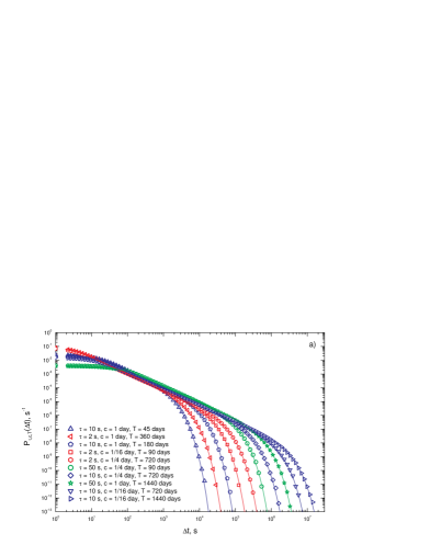
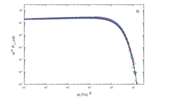
Figure 1: a) Inter-occurrence time distributions for the NHP process with the decaying rate (3). Symbols are numerical simulations of the NHP process. Solid lines are numerical integrations of Eq. (2). b) The scaling analysis of the distributions for $\Delta t\geq 150$ s using Eq. (4). The solid line is a fit of the generalized gamma function to the rescaled data.

In Fig. 1a we show plots of numerical simulations of the NHP process with varying scaling parameters $\tau$, $c$, and $T$ with fixed $p=1.2$. These are indicated as solid symbols. We also plot the corresponding numerical integrations of Eq. (2) for the same values of $\tau$, $c$, and $T$. The comparison shows that Eq. (2) correctly describes the inter-occurrence time distributions between events.

We have also performed a scaling analysis of our simulated distributions for the values $\Delta t\geq 150$ s. This is shown in Fig. 1b. The distributions collapse onto each other with respect to the following scaling law

$$P_{\tau,c,T}(\Delta t)=\frac{1}{\tau}\,\left(\frac{\Delta t}{\tau}\right)^{-\alpha}\,f\left[\frac{\Delta t}{\tau}\,\left(\frac{T}{c}\right)^{-\beta}\right]\,,$$ (4)

where $\alpha=1.212$ and $\beta=1.194$. The scaling function $f(x)$ can be approximated by the generalized gamma function $f(x)=A\,x^{\gamma}\,\exp(-x/B)$ with $\gamma=0.056$, $A=0.329$, and $B=1.122$. The distribution functions have two characteristic time-scales, i.e. $\tau$ and $\tau(T/c)^{\beta}$, which define two roll overs for small and large $\Delta t$’s.

To find scaling relations between the above exponents, one has to perform an asymptotic analysis of the integral (2) for large $\Delta t\gg 1$ and $T\gg 1$. This analysis can be done by using Laplace’s method Olver (1974) and gives $P(\Delta t)\sim{\Delta t}^{-(2-1/p)}$ for $T\to\infty$ and $P(\Delta t)\sim\exp[-\Delta t/\tau(1+T/c)^{p}]$ for finite $T$, from which we conclude that $\alpha-\gamma=2-1/p$ and $\beta=p$. The exponent $2-1/p$ was also reported in Utsu et al. (1995).

To check the proposed hypothesis that aftershocks can be modeled as a NHP process, the derived distribution (2) has been compared to several aftershock sequences in California. We have used the seismic catalog provided by the Southern California Earthquake Center (SCSN catalog, http://www.data.scec.org). The identification of aftershock sequences is usually an ambiguous problem which requires assumptions on the spatial and temporal clustering of aftershocks Kisslinger (1996). In this work we assume that all events that have occurred after a main shock within a given time interval $T$ and a square area $L\times L$ are aftershocks of a particular main shock. By neglecting the magnitude, spatial size and duration of each individual event and considering all aftershocks above a certain threshold $m_{c}$, we map a multi-dimensional process into a process on the one-dimensional time-line. This marked process is characterized by the times of occurrence of individual events $t_{i}$ and their magnitudes $m_{i}$. We define inter-occurrence or waiting times between successive aftershocks as $\Delta t_{i}=t_{i}-t_{i-1}$, $i=1,2,\ldots$ and study their statistical distribution over a finite time interval $T$.

In this work, we use the decay rate of aftershocks, introduced in Shcherbakov et al. (2004, 2005), which is a generalization of the modified Omori’s law (3), where the characteristic time $c(m)=\tau\,(p-1)\,10^{b\,(m^{\star}-m)}$ is a function of the lower cutoff magnitude of an aftershock sequence $m$, $m^{\star}$ is the maximum value of an aftershock in a sequence with finite number of events, and $p>1$. We also assume that aftershock sequences satisfy the Gutenberg-Richter cumulative distribution $N(\geq m)=10^{b\,(m^{\star}-m)}$. This defines a truncated distribution where the expected number of events with magnitudes greater than $m^{\star}$ is equal to one and the exponent $b$ is generally near unity Shcherbakov and Turcotte (2004).

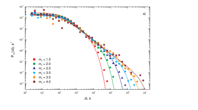
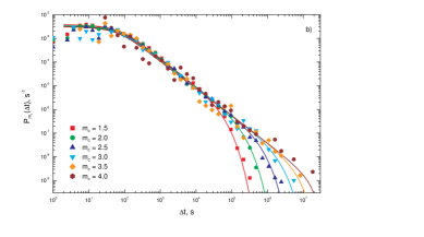
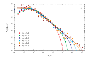
Figure 2: Inter-occurrence time distributions for the three California aftershock sequences for different magnitude cutoffs $m_{c}=1.5,2.0,2.5,\dots,4.0$. Square areas considered are $1.25^{\circ}\times 1.25^{\circ}$ for (a) the Landers sequence and $1.0^{\circ}\times 1.0^{\circ}$ for (b) the Northridge and (c) Hector Mine sequences each centered on the epicenters of the main shocks. In all cases a time interval of $T=1$ year following the main shock has been used. The solid lines have been computed using Eq. (2).

In Fig. 2 we have computed the distribution functions of inter-occurrence times between successive aftershocks from the observed data of three California aftershock sequences. These are indicated as solid symbols in Fig. 2. For each of these sequences we have used square boxes of size $L\times L=1.25^{\circ}\times 1.25^{\circ}$ for the Landers earthquake ($m_{ms}=7.3$; Jun 28, 1992) and $1.0^{\circ}\times 1.0^{\circ}$ for the Northridge ($m_{ms}=6.7$; Jan 17, 1994) and Hector Mine ($m_{ms}=7.1$; Oct 16, 1999) earthquakes centered on the epicenter of the main shocks and a time interval of $T=1$ year. All the earthquakes that occurred in the spatio-temporal boxes were treated as aftershocks. The analysis of the data shows that the distributions are not too sensitive to changes in the linear size $L$ of the box, the results are almost the same for $L$ ranging from $0.25^{\circ}$ to $1.75^{\circ}$ within statistical errors. This means that the distributions are dominated by the activity of the events generated by the main shocks and the background seismicity doesn’t contribute significantly to the scaling.

In this analysis of an aftershock sequence as a point process we treat all earthquakes as having the same magnitude and as a result we lose a significant fraction of information related to the physics of the process. To recover some information from the magnitude domain of each sequence we have used a lower magnitude cutoff $m_{c}$ as a scaling parameter and study sequences with different $m_{c}$’s. These are depicted by different colors in the plots (Fig. 2). The distributions with lower magnitude cutoffs have a shorter power-law scaling regime and start to roll over more quickly. This can be explained by the presence of more events in the sequences with lower magnitude cutoffs and as a result the shortening of the mean time intervals between events. Another scaling parameter which affects the roll over is the time interval $T$. An increase in $T$ leads to the occurrence of longer intervals $\Delta t$ between events.

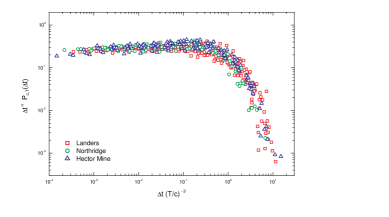
Figure 3: The scaling analysis of the inter-occurrence time distributions of the three aftershocks sequences according to (4). The red, green, and blue symbols correspond to the Landers ($p=1.22$, $\tau=107.25$ s), Northridge ($p=1.17$, $\tau=53.14$ s), and Hector Mine ($p=1.22$, $\tau=83.71$ s) sequences. In each sequence the varying parameters $c$ and $T=180$, $360$, and $720$ days have been used. The best collapse have been found for $\alpha=1.25$ and $\beta=1.22$.

To compare the observed scaling with the simulations of a NHP process we also plot in Fig. 2, as solid curves, the distributions computed assuming that aftershock sequences follow NHP statistics with the rate given by Eq. (3) and the parameters $\tau$, $c$, and $p$ estimated from the observed three California aftershock sequences Shcherbakov et al. (2004). The plots show that the modeled distributions are in excellent agreement with the observations.

We have also performed a scaling analysis of the inter-occurrence time distributions of these aftershock sequences. This is shown in Fig 3. The characteristic time $c$ and the time interval $T$ have been chosen as scaling parameters. These sequences are characterized by slightly different initial rates $\tau$ and exponents $p$. The results show a reasonably good scaling with respect to $c$ and $T$ which supports our hypothesis that aftershock sequences can be described as a NHP process.

In summary, the studies of inter-occurrence of aftershocks presented in this work suggest that aftershock sequences can be modeled to a good approximation as a point process governed by NHP statistics, where the rate of activity decays as a power-law (Eq. 3). This decaying rate introduces a self-similar regime into the observed scaling followed by an exponential roll over. An analysis of a nonstationary earthquake sequence was also performed in Corral (2005). It was suggested the existence of a secondary clustering structure within the main sequence and deviation from NHP behavior. The knowledge of the type of distribution that governs the occurrence of aftershocks is important in any hazard assessment programs. The derived distribution (Eq. 2) has much broader applicability and can be used for studies of many time dependent processes which follow NHP statistics.

Fruitful discussions with A. Corral and A. Soshnikov are acknowledged. The comments of the anonymous reviewer helped to enhance the analysis. This work has been supported by NSF grant ATM 0327558 (DLT, RS) and US DOE grant DE-FG02-04ER15568 (RS, GY, JBR).

References

- Rundle et al. (2003) J. B. Rundle, D. L. Turcotte, R. Shcherbakov, W. Klein, and C. Sammis, Rev. Geophys. 41, Art. No. 1019 (2003).
- Vere-Jones (1970) D. Vere-Jones, J. Roy. Statist. Soc. B 32, 1 (1970).
- Ogata (1999) Y. Ogata, Pure Appl. Geophys. 155, 471 (1999).
- Daley and Vere-Jones (2002) D. J. Daley and D. Vere-Jones, An Introduction to the Theory of Point Processes, vol. 1 (Springer, New York, 2002).
- Kisslinger (1996) C. Kisslinger, in Advances in Geophysics (Academic Press, San Diego, 1996), vol. 38 of Advances in Geophysics, pp. 1–36.
- Gutenberg and Richter (1954) B. Gutenberg and C. F. Richter, Seismicity of the Earth and Associated Phenomenon (Princeton Univiversity Press, Princeton, 1954), 2nd ed.
- Utsu et al. (1995) T. Utsu, Y. Ogata, and R. S. Matsu’ura, J. Phys. Earth 43, 1 (1995).
- Robertson et al. (1995) M. C. Robertson, C. G. Sammis, M. Sahimi, and A. J. Martin, J. Geophys. Res. 100, 609 (1995).
- Davidsen and Goltz (2004) J. Davidsen and C. Goltz, Geophys. Res. Lett. 31, Art. No. L21612 (2004).
- Bak et al. (2002) P. Bak, K. Christensen, L. Danon, and T. Scanlon, Phys. Rev. Lett. 88, Art. No. 178501 (2002).
- Corral (2003) A. Corral, Phys. Rev. E 68, Art. No. 035102 (2003).
- Lindman et al. (2005) M. Lindman, K. Jonsdottir, R. Roberts, B. Lund, and R. Bodvarsson, Phys. Rev. Lett. 94, Art. No. 108501 (2005).
- Corral (2004a) A. Corral, Phys. Rev. Lett. 92, Art. No. 108501 (2004a).
- Corral (2004b) A. Corral, Physica A 340, 590 (2004b).
- Corral (2005) A. Corral, Nonlinear Process Geophys. 12, 89 (2005).
- Mega et al. (2003) M. S. Mega, P. Allegrini, P. Grigolini, V. Latora, L. Palatella, A. Rapisarda, and S. Vinciguerra, Phys. Rev. Lett. 90, Art. No. 188501 (2003).
- Yakovlev et al. (2005) G. Yakovlev, J. B. Rundle, R. Shcherbakov, and D. L. Turcotte (2005), cond–mat/0507657.
- Olver (1974) F. W. J. Olver, Asymptotics and Special Functions (Academic Press, New York, 1974).
- Shcherbakov et al. (2004) R. Shcherbakov, D. L. Turcotte, and J. B. Rundle, Geophys. Res. Lett. 31, Art. No. L11613 (2004).
- Shcherbakov et al. (2005) R. Shcherbakov, D. L. Turcotte, and J. B. Rundle, Pure Appl. Geophys. 162, 1051 (2005).
- Shcherbakov and Turcotte (2004) R. Shcherbakov and D. L. Turcotte, Bull. Seismol. Soc. Am. 94, 1968 (2004).