Thermodynamics and equilibrium structure of Ne₃₈ cluster: Quantum Mechanics versus Classical

Abstract

The equilibrium properties of classical LJ₃₈ versus quantum Ne₃₈ Lennard-Jones clusters are investigated. The quantum simulations use both the Path-Integral Monte-Carlo (PIMC) and the recently developed Variational-Gaussian-Wavepacket Monte-Carlo (VGW-MC) methods. The PIMC and the classical MC simulations are implemented in the parallel tempering framework. The classical heat capacity $C_{v}(T)$ curve agrees well with that of Neirotti et al [J. Chem. Phys. 112, 10340 (2000)], although a much larger confining sphere is used in the present work. The classical $C_{v}(T)$ shows a peak at about 6 K, interpreted as a solid-liquid transition, and a shoulder at $\sim$4 K, attributed to a solid-solid transition involving structures from the global octahedral ($O_{h}$) minimum and the main icosahedral ($C_{5v}$) minimum. The VGW method is used to locate and characterize the low energy states of Ne₃₈, which are then further refined by PIMC calculations. Unlike the classical case, the ground state of Ne₃₈ is a liquid-like structure. Among the several liquid-like states with energies below the two symmetric states ($O_{h}$ and $C_{5v}$), the lowest two exhibit strong delocalization over basins associated with at least two classical local minima. Because the symmetric structures do not play an essential role in the thermodynamics of Ne₃₈, the quantum heat capacity is a featureless curve indicative of the absence of any structural transformations. Good agreement between the two methods, VGW and PIMC, is obtained. The present results are also consistent with the predictions by Calvo et al [J. Chem. Phys. 114, 7312 (2001)] based on the Quantum Superposition Method within the harmonic approximation. However, because of its approximate nature, the latter method leads to an incorrect assignment of the Ne₃₈ ground state as well as to a significant underestimation of the heat capacity.

I Introduction.

In this paper, we investigate equilibrium properties of the Ne₃₈ Lennard-Jones (LJ) cluster. Particularly, we are interested in how the equilibrium structure, energy, and heat capacity as functions of temperature are affected by the quantum nature of the system. Our interest is partly motivated by recent advances in the development of accurate numerical Quantum Statistical Mechanics techniques as well as by their successful applications to smaller Lennard-Jones clusters. As such, Refs. HCest report fully converged heat capacity curves obtained by the Path-Integral Monte-Carlo (PIMC) method for various Ar_13-nNe_n Lennard-Jones clusters. The $\mathrm{LJ}_{13}$ cluster is one of the smallest that exhibits a pronounced liquid-solid-like structural transition, according to the existence of a peak in the heat capacity curve $C_{v}(T)$. On the other hand, $\mathrm{Ne}_{13}$ is perhaps the largest Ne cluster treated so far quantum mechanically on the entire range of interesting temperatures HCest ; Examples_Ne13 .

In the case of Ar or heavier rare gas clusters, the quantum effects can safely be treated as small perturbations C_T . However, it has long been known that the Ne clusters exhibit strong quantum effects, not only in the low temperature regime, but also in liquid phase Old_Ne . Still, perhaps because $7$ and $13$ are magic numbers, the quantum effects do not essentially change the structural or thermodynamic properties of the respective Ne clusters. For example, although the heat capacity $C_{v}(T)$ around the “solid-liquid” transition temperature ($T\sim$ 10 K) is reduced in magnitude and shifted about $10\%$ toward lower temperatures as compared with the purely classical LJ₁₃, the heat capacity curve for Ne₁₃ has a behavior similar to that of LJ₁₃. It would certainly be interesting to verify whether the quantum effects lead or not to qualitative differences for larger Ne clusters, especially those that do not have a magic number of particles. Of particular interest is the $\mathrm{Ne}_{38}$ cluster, for which there is the additional question of whether or not the quantum ground state is still localized in the celebrated octahedral basin, a basin that contains the classical global minimum MinLJ38 and which represents a deviation from the icosahedral Mackay packing characteristic of all the other neighboring clusters Northby .

An attempt to answer these questions for a variety of rare gas LJ clusters (including Ne₃₈) has been made by Calvo, Doye, and Wales C_T , using various approximations, particularly, the quantum superposition method. In this approximation, one treats all the classical minima of the potential energy surface independently and within an harmonic approximation. Quite interestingly, the technique predicts the absence of the solid-liquid transition peak in the heat capacity curve for the quantum Ne₃₈ cluster. Also, it suggests that the global minimum is no longer localized in the octahedral basin. However, although many of the conclusions of Ref. C_T remain qualitatively unchanged, we have found that the energy estimates given by the harmonic approximation in this case are unacceptably inaccurate. For instance, the harmonic approximation incorrectly assigns the ground state to a state from the icosahedral basin (state $4$ from Table 1) that turns out to have an energy about $24.6~{}k_{\mathrm{B}}\mathrm{K}$ greater than the octahedral-based structure, invalidating the conclusions of Ref. C_T . Nevertheless, we still find that the configurations of minimum quantum-mechanical energy are indeed disordered, liquid-like structures localized in the icosahedral basin. Yet, it is clear that techniques that are more sophisticated than the Quantum Superposition Method must be utilized for a reliable study of the thermodynamic and structural properties of the Ne clusters. As Calvo, Doye, and Wales acknowledge, it would be desirable if their results could be verified by more accurate simulations, although they note: “It is very likely that simulating $\mathrm{LJ}_{31}$ or $\mathrm{LJ}_{38}$ by quantum Monte Carlo methods at thermal equilibrium is not practical with the current computer technology.” We attempt to give a partial answer to their challenge by utilizing two different quantum algorithms, both of which have been shown to accurately treat the smaller $\mathrm{Ne}_{13}$ cluster HCest ; Neon13 .

The first algorithm is a random series based PIMC technique RandomSeries ; Pre04a ; Pre04b which, in principle, is an exact method. It must be realized though that an accurate computation of the heat capacity is a more demanding task for PIMC than the evaluation of the average energy, for instance. Even for the latest heat capacity estimators HCest , the standard deviation still grows as fast as $T^{-2}$, when the temperature is lowered (the prediction is a theoretical upper bound; in practice, we have always observed an improved behavior, closer to $T^{-1}$). At the same time, the heat capacity itself decreases at a rate following perhaps a polynomial law for a large range of low temperatures C_T (of course, after removing the part associated with the translational degrees of freedom, the decrease is exponentially fast in the extreme low temperature limit, due to the finite number of particles in the cluster). Thus, the relative error increases rather severely at low temperatures. Other limitations of the PIMC method come from the increase in the numerical effort associated with the larger number of path variables needed for low temperatures as well as from the sampling difficulties related to the larger number of path variables. However, the latter kind of limitations are surmountable, either by employing path integral techniques having faster asymptotic convergence Pre04a ; PIMC_fast or by employing better sampling strategies Pre04b ; PIMC_sampling . Most likely, the biggest gain will come from the design of better heat capacity estimators. To cope with ergodicity problems, the path integral technique has been utilized in conjunction with the parallel tempering procedure paral_temp , in which a number of Metropolis walks at different temperatures are utilized, with the configurations generated by walks with similar temperatures swapped periodically.

In Refs. gauss_CPL ; Neon13 a novel method (VGW-MC) using variational Gaussian wavepackets in conjunction with a Monte Carlo sampling of the initial conditions was developed and tested for various benchmark systems including the Ne₁₃ Lennard-Jones cluster. The original Heller’s idea of using the VGW’s for approximate solution of the time-dependent Schrödinger equation Heller_JCP75 ; Heller_JCP76 was later followed by many groups. Some important, but certainly not complete references are frozen_gauss ; Metiu_many_gauss ; metiu_dens ; Coalson ; G-MCTDH ; Coalson_fly ; QMD_review ; Martinez ; Buch . While most of the developments were concerned with the real-time dynamics, the work of Metiu and co-workers metiu_dens , where the VGW’s were adapted to the solution of the “imaginary-time” Schrödinger equations, most closely relates to the present VGW-MC method.

The VGW-MC is a manifestly approximate quantum statistical mechanics approach, which is supposed to be exact only in the high temperature limit or for a purely harmonic system. Quite surprisingly, the results obtained by this method for general strongly unharmonic systems turned out to be very accurate, even at low temperatures. For example, in the case of the Ne₁₃ cluster, nearly quantitative agreement with the existing PIMC calculations was achieved for the heat capacity and equilibrium structural properties. Although the method does employ Monte Carlo sampling, its convergence properties at low temperatures are completely different from those in the parallel tempering Monte Carlo schemes: the initial conditions for the Gaussian wavepackets are sampled by a primitive Metropolis walk running at an inverse temperature $\beta=\beta_{\rm MC}$ sufficiently small to ensure ergodicity. Each Gaussian is then propagated to the higher values of $\beta$ making its contribution to the partition function. Thus, a single Metropolis walk is used to obtain results for the entire temperature range of interest, also circumventing the quasi-ergodicity problems at low temperatures. As argued and demonstrated in Ref. Neon13 , it is the quantum nature of the Ne system which ensures the convergence of the method, a convergence that, at first glance, may seem completely counterintuitive. Some numerical aspects of the VGW-MC method still remain to be explored in the future. Those include the use of more efficient sampling strategies. For instance, the method can be implemented in the parallel tempering fashion if needed. However, since the numerical scheme, as described in Ref. Neon13 , worked for the present case of the Ne₃₈ cluster, no attempts to optimize its performance were made here. Thus, in the present study, the computations are done using both parallel tempering PIMC and VGW-MC. The latter approach seems to have better convergence properties at low temperatures, while the former is manifestly exact (when the statistical errors can be made sufficiently small).

The double-funnel topology of the potential energy surface of the $\mathrm{LJ}_{38}$ cluster Ne38_double-funnel has proved a tough simulation challenge for most of the Monte Carlo algorithms. This challenge has only recently been answered by Neirotti and coworkers Neirotti_Ne38 , who have employed the parallel tempering algorithm to successfully simulate a $\mathrm{LJ}_{38}$ cluster confined by a hard-wall potential with a radius of $R_{c}=2.25~{}\sigma_{\rm LJ}$. Extensive studies made by Neirotti and coworkers have shown that the parallel tempering algorithm in the canonical ensemble cannot equilibrate the $\mathrm{LJ}_{38}$ cluster in about $100$ million passes through the configuration space, if the original Lee, Barker, and Abraham conf_R confining radius of $R_{c}=3.612\;\sigma_{\rm LJ}$ is utilized. However, they have argued that the thermodynamics of the cluster remains basically unchanged if a smaller confining radius of $R_{c}=2.25\;\sigma_{\rm LJ}$ is utilized.

For the quantum $\mathrm{Ne}_{38}$ cluster the confining radius of $R_{c}=2.25\sigma_{\rm LJ}$ is perhaps too small. For instance, the radius of the configuration proposed in Ref. C_T as a ground state for the $\mathrm{Ne}$ cluster (state 4 in Table 1) is $R_{c}=2.255\sigma_{\rm LJ}$, after quenching to the closest classical minimum. Clearly, such a state would have been made inaccessible by the small confining radius utilized by Neirotti et al. In the present work, we utilize a confining potential in the form of a steep polynomial, which is more suitable for quantum simulations. It has been argued that, for such an analytical form of the confining potential, a larger confining radius of at least $R_{c}=2.65~{}\sigma_{\rm LJ}$ is necessary in order to ensure that the low-temperature thermodynamic properties of the classical cluster are not significantly altered Freeman_preprint . For quantum systems, one needs to worry about the possibility that the effects of quantum delocalization may lead to an even stronger influence of the confining radius on the structural properties of the $\mathrm{Ne}_{38}$ cluster. Thus, in the present study we have decided to employ the original confining radius of $R_{c}=3.612\;\sigma_{\rm LJ}$. In making this choice, we have been also motivated by the preliminary findings that the large quantum effects, through raising the zero-point energies and barrier tunneling, radically reduce the difficulty of the sampling problem. Yet, we had to make sure that the thermodynamic and structural changes observed are solely due to quantum effects and not to the larger confining radius employed. For this reason, we have started our investigation with a Monte Carlo simulation for the classical $\mathrm{LJ}_{38}$ cluster, which is presented in the following section.

II Parallel tempering simulation of the $\mathrm{LJ}_{38}$ cluster

As discussed in the Introduction, the first successful attempts Neirotti_Ne38 to compute the thermodynamic properties of the $\mathrm{LJ}_{38}$ cluster by parallel tempering simulations have revealed the difficulty in attaining ergodicity. The $\mathrm{LJ}_{38}$ cluster has a double-funnel topology of the potential energy surface Ne38_double-funnel , with the octahedral and icosahedral basins separated by a large-energy barrier. The way parallel tempering paral_temp tries to overcome the high-energy barrier is by coupling a set of statistically independent Monte Carlo Markov chains via exchanges of configurations between replicas of slightly different temperatures. The swapping events by themselves do not lead to new configurations. Rather, the configurations from the low-temperature replicas climb the ladder of temperatures and reach the high-temperature replicas, where they are destroyed and replaced with energetically more favorable configurations.

The rate of equilibration of the parallel-tempering simulation depends on the ability of the high-temperature Metropolis walkers to jump between the icosahedral and the octahedral basins with a sufficiently high frequency. Let us mention that, although they have enough energy to do so, the replicas of highest temperature must defeat the action of the entropy, which favors the configurations from the icosahedral basin or, beyond the melting point, the configurations that are associated with the liquid phase. At high temperature, the number of local minima that become thermodynamically accessible increases as $\sim\exp(\alpha N)$ (not counting the permutationally symmetric configurations), with the dimensionality $N$ of the cluster local_minima . Therefore, the ability of the high-temperature replicas to find configurations in the octahedral basin (the basin associated with the global minimum) is quite low and decreases further if the vapor pressure of the cluster is decreased, for instance, by increasing the confining radius. As such, the finding of Neirotti et al Neirotti_Ne38 that the system is hard to equilibrate even in $100$ million passes must not necessarily come as a surprise.

The Lennard-Jones parameters utilized in this paper are those employed in previous studies of Ne clusters HCest : $\epsilon_{\rm LJ}=35.6$ K and $\sigma_{\rm LJ}=2.749$ A. The mass of Ne atom was assumed to be $m=20$ a.u. In both classical and PIMC simulations, we have employed the same analytical expression for the confining potential, in the form of the steep polynomial

$$V_{c}(\mathbf{r_{i}})=\epsilon_{\rm LJ}\left({\|\mathbf{r_{i}}-\mathbf{R_{cm}}\|}/{R_{c}}\right)^{20}.$$ (1)

Here, $\mathbf{R_{cm}}$ is the center of mass, whereas $R_{c}=3.612~{}\sigma_{\rm LJ}$ is the confining radius. Recent studies performed by Sabo, Freeman, and Doll Freeman_preprint have demonstrated that low-temperature thermodynamic properties of the cluster may be sensitive not only to the exact value of the confining radius, but also to the shape of the potential. Because the polynomial potential is not sufficiently flat for small values of $\|\mathbf{r_{i}}-\mathbf{R_{cm}}\|$ when compared to a hard-wall potential, a radius of at least $R_{c}=2.65~{}\sigma_{\rm LJ}$ must be utilized in order to prevent the disappearance of the pre-melting solid-solid phase change Freeman_preprint . However, beyond this radius, the vapor pressure depends only slightly on the exact value of the confining radius, for a large range of such values. The low-temperature thermodynamic properties and, to a good extent, the properties of the liquid phase remain invariant to the exact value of the confining radius. Nevertheless, the confining radius of $R_{c}=2.65~{}\sigma_{\rm LJ}$, which is a minimal requirement for a classical cluster, is no longer satisfactory for the quantum $\mathrm{Ne}_{38}$ cluster, whence our decision to employ the significantly larger Lee, Barker, and Abraham value of $R_{c}=3.612~{}\sigma_{\rm LJ}$ appears justified, although not computationally optimal in the sense of Ref. Freeman_preprint .

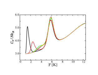
Figure 1: Evolution of the heat capacity profiles for the $\mathrm{LJ}_{38}$ cluster during the parallel tempering Monte Carlo simulation. Each of the six curves has been computed by collecting averages for successive groups of $50$ million passes. Early on in the simulation, the heat capacity shows a fake maximum at low temperatures, maximum that is gradually washed out and transformed in a “shoulder.” The last two curves are virtually indistinguishable on the plot and the data utilized to compute them have also been employed for the final result.

We have employed exactly the same parallel tempering strategy as the one from Neirotti et al Neirotti_Ne38 , except for a larger number of parallel replicas, $64$ instead of $40$, which have been arranged in a geometric progression spanning the interval of temperatures $[1.0~{}\mathrm{K},12.46~{}\mathrm{K}]$. As such, we do not describe the technique here and, instead, refer the reader to the cited reference. To begin with, we have performed a first simulation in $100$ million sweeps (passes) through the configuration space, which were preceded by $20$ million warming steps. The sweeps have been divided in blocks of $5$ million each. Rather than using all $20$ blocks to compute the heat capacity, we have calculated two heat capacity curves, each using $10$ blocks of data. This approach allows us to evaluate the convergence of the simulation. The two curves are those from Fig. 1 that exhibit a clearly defined low-temperature maximum, additional to the one associated with the solid-liquid transition.

The appearance of the fake low-temperature peak in the heat capacity curves early in the simulation tells us a lot about how parallel tempering works. Such peaks are due to solid-solid transitions between the configurations from the octahedral and the icosahedral basins, transitions that lead to large energy fluctuations. The transitions between the replicas are achieved through the replica exchange mechanism. Because at the beginning of the simulation only a few octahedral configurations have been found, a low temperature replica is forced to jump between octahedral and icosahedral configurations through the exchange mechanism. As the simulation goes on, more and more octahedral configurations are found. Because they are energetically more stable, they are placed in the replicas of lower energy. These low-temperature replicas are involved more and more only in exchanges of configurations from the octahedral basin and their energy fluctuations decrease: the fake heat capacity peak moves to higher temperatures.

Figure 2: Heat capacity per atom in units of $k_{B}$ for the $\mathrm{LJ}_{38}$ cluster using a confining radius of $R_{c}=3.612\sigma_{\rm LJ}$. In the lower panel, the derivative against temperature is given. As explained by Neirotti and coworkers Neirotti_Ne38 , the small low temperature maximum in the derivative curve is associated with a second order solid-solid phase transition between the configurations from the octahedral and icosahedral basins.

The mechanism described in the preceding paragraph also implies that the rate of equilibration of the parallel tempering simulation can be estimated from the rate at which the fake maxima move to the right. More precisely, because the supply of newly found octahedral configurations is steady, the peaks will move to the right roughly at a constant rate until the heat capacity profile reaches the equilibrium shape. Based on this line of reasoning, we have performed two more simulations of $100$ million passes, each preceded by $20$ million warming sweeps, and each starting from the last configuration of the previous simulation. The four heat capacity curves generated using the new data are also shown in Fig. 1, with the last two being virtually indistinguishable. The data obtained in the last $100$ million passes have been utilized to compute the heat capacity curve from Fig. 2. Thus, the simulation has needed about $260$ million passes for the equilibration phase and only $100$ million for the accumulation phase.

The heat capacity curve obtained is almost identical to the one computed by Neirotti and coworkers. Thus, our simulation constitutes a direct proof of their assertion that the constraining radius of $R_{c}=2.25\sigma_{\rm LJ}$ is large enough not to essentially change the low-temperature thermodynamics of the cluster. On the other hand, our simulation reveals a very important property of the parallel tempering algorithm. If the high-temperature replicas are capable of finding the relevant configurations at a reasonable rate, then the simulation will converge quite quickly and it should not be stopped prematurely. Future research in the development of replica exchange techniques should be concerned with designing ways to identify which of the replicas generate the bottleneck configurations and how one can improve the rate at which the configurations are generated.

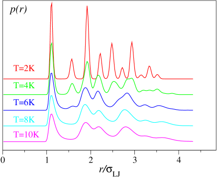
Figure 3: Radial pair correlation functions for the classical LJ₃₈ cluster. Notice the change in the number and the position of peaks, as the temperature is lowered from $T=10~{}\mathrm{K}$ (liquid phase), to $T=6~{}\mathrm{K}$ (mainly structures from the icosahedral basin), and finally to $T=2~{}\mathrm{K}$ (mainly structures from the octahedral basin).

In Fig. 3, we present the radial pair correlation functions for different temperatures. The shape of the functions changes as the temperature is lowered from $T=10~{}\mathrm{K}$, which contains configurations characteristic of the liquid phase, to $T=6~{}\mathrm{K}$, which mainly contains structures from the icosahedral basin, and finally to $T=2~{}\mathrm{K}$, which mainly contains structures from the octahedral configurations. The association of the shape of the radial pair correlation functions with the respective configurations is based upon the analysis of several order parameters performed by Neirotti and coworkers. (Also see below the comparison of classical and quantum $p(r)$ of the same symmetries.)

III The Path Integral Monte Carlo technique

It has been long recognized that the computation of heat capacities by path integral Monte Carlo techniques is quite difficult, due to the strong decrease in the heat capacity with the decrease in the temperature. Our ability to report well-converged PIMC results for relatively low temperatures (down to $1.78~{}\mathrm{K}$ for the $\mathrm{Ne}_{38}$ cluster) relies on recent developments in the design of direct path integral techniques (techniques that solely call the potential function for the evaluation of physical properties). Such developments include: short-time approximations having faster asymptotic convergence Pre04a , more efficient sampling techniques Pre04b , and thermodynamic energy and heat capacity estimators having lower variances RandomSeries ; HCest . Because the PIMC technique has been extensively described in the cited references, here, we only enumerate its salient features.

We employ a finite-dimensional approximation to the Feynman-Kac formula in the form of a Lie-Trotter product

$$\rho_{n}(x,x^{\prime};\beta)=\int_{\mathbb{R}}dx_{1}\ldots\int_{\mathbb{R}}dx_{n}\;\rho_{0}\left(x,x_{1};\frac{\beta}{n+1}\right)$$

$$\ldots\rho_{0}\left(x_{n},x^{\prime};\frac{\beta}{n+1}\right)$$ (2)

of a short-time approximation of the type

$$\rho_{0}(x,x^{\prime};\beta)=\rho_{fp}(x,x^{\prime};\beta)\int_{\mathbb{R}}d\mu(a_{1})\cdots\int_{\mathbb{R}}d\mu(a_{3})$$

$$\times\exp\left\{-\beta\sum_{i=1}^{4}w_{i}V\left[x_{r}(u_{i})+\sigma\sum_{k=1}^{3}a_{k}\tilde{\Lambda}_{k}(u_{i})\right]\right\}.$$ (3)

The quadrature points $u_{i}$ and weights $w_{i}$ as well as the functions $\tilde{\Lambda}_{k}(u)$ are designed such that the convergence

$$\rho_{n}(x,x^{\prime};\beta)\to\rho(x,x^{\prime};\beta)$$

is as fast as $O(1/n^{4})$. These parameters are universal, in the sense that they are independent of the choice of potential $V(x)$, and are given in Ref. Pre04a , reference that should be consulted for further information. Here, we only mention that the short-time approximation introduces additional path variables. The total number of path variables for the diagonal elements of the $n$-th order Lie-Trotter product is $4n+4$, which is the number we report. The number of evaluations of the potential function necessary to compute the action for a particular path parameterized by the $4n+4$ path variables is also $4n+4$. Therefore, the computational effort relative to the number of path variables is the same as for the trapezoidal Trotter approximation, yet the technique has a superior asymptotic convergence, $O(1/n^{4})$, as opposed to $O(1/n^{2})$.

The Monte Carlo procedure is based on the fast sampling algorithm. As observed in Ref. Pre04b , updating more than a few path variables at a time in a Metropolis step results in a decrease in the maximal displacements that is proportional to the square root of the number of path variables updated. The effect is entropic in nature and is roughly independent of the amount of correlation between the variables that are sampled. On the other hand, if the variables are updated separately, one needs to perform $4n+4$ potential evaluations for each of the $4n+4$ variables. It has been argued that the number of potential evaluations for an efficient update of the path variables scales as $(4n+4)^{2}$, regardless of the strategy utilized. The fast sampling algorithm is based on the observation that, if $n=2^{k}-1$, then the $4n+4$ variables can be divided in $4+\log_{2}(n+1)$ layers, with the path variables from each layer being statistically independent. With a single evaluation of the action, one can update all variables from a layer, independently. Therefore, the cost to update all path variables in a statistically efficient manner is $(n+1)[4+\log_{2}(n+1)]$, a significantly better scaling.

Numerical experiments have shown that the number of path variables necessary to achieve systematic errors comparable to the statistical errors is $4n+4=256$. The number of layers is $10$. A total of $10\times 256=2560$ potential evaluations are needed to efficiently update each of the path variables associated with a given degree of freedom. Similar to the Monte Carlo simulation for the classical system, the path variables corresponding to different particles are updated separately. We have randomly selected a particle and a layer and updated the corresponding path variables. It follows that a pass or sweep through the configuration space requires $38\times 10=380$ elementary Metropolis steps. The simulation employed for the computation of the heat capacity curve has consisted of $100$ accumulation blocks of $2$ thousand passes each. The accumulation phase has been preceded by $50$ equilibration blocks. The Monte Carlo replicas corresponding to different temperatures have been involved in exchanges of configurations each $2$ passes, according to the parallel tempering algorithm. We have employed a number of $64$ independent replicas of temperatures arranged in a geometric progression spanning the interval $[1.78~{}\mathrm{K},12.46~{}\mathrm{K}]$. The observed acceptance rates for replica exchanges were larger than $40\%$.

The thermodynamic energy and heat capacity estimators are those obtained by formal differentiation of the Lie-Trotter formula RandomSeries . The temperature differentiation can be performed by a central finite-difference scheme requiring three points HCest . Thus, the overall computational effort for the quantum simulation is a factor of $3\times 2560=7680$ larger than for the classical simulation, per Monte Carlo sweep. Fortunately, because of the extensive quantum effects, one does not need so many passes as for the classical simulation. In fact, as our later results show, the configurations associated with the octahedral basin, which contains the classical global minimum, have an unfavorable quantum energy. The effective topology of the potential energy surface is drastically simplified, with the octahedral basin being almost completely taken out of the picture. Therefore, the ergodicity problems observed for the classical simulation do not appear in the case of the quantum simulation.

In addition to the main Monte Carlo simulation, we have performed several Monte Carlo simulations at the fixed temperature of $T=1.78~{}\mathrm{K}$, in order to estimate the average energy of the configurations of minimal energy from Table 1. These simulations have utilized $4$ parallel streams of $50$ blocks each, for a total of $200$ accumulation blocks. The accumulation phase has been preceded by $25$ equilibration blocks. The simulations have been started from the centers of the Gaussian wavepackets of minimal energy that were obtained during the VGW simulation. We did not utilize parallel tempering for these simulations because globally ergodic walkers would eventually leave the starting configurations and move to entropically more favorable configurations. Only through broken ergodicity can we meaningfully associate the estimated energies with the input configurations. To verify the association, we have quenched several of the final positions of the simulated configurations. In all cases, we have recovered with a high probability (over $50\%$) the initial configurations. However, for both of the configurations $1$ and $2$, we have obtained another classical minimum, the basin of which was frequently visited. Thus, at least for the temperature of $1.78~{}\mathrm{K}$, the configurations of lowest energy are delocalized over basins associated with at least two classical minima.

IV VGW-MC: Variational-Gaussian-Wavepacket Monte-Carlo.

A general and detailed description of the VGW-MC method can be found in Ref. Neon13 . In this section, we summarize those aspects of the technique that regard the calculation of the partition function for a $N$-particle system,

$$Z:=\mbox{Tr}\ \exp(-\beta\widehat{H})$$

with $\beta=1/k_{\rm B}T$. The equilibrium energy is computed by differentiating the partition function

$$E=k_{\rm B}T^{2}\frac{\partial\mbox{ln}Z}{\partial T},$$ (4)

whereas the heat capacity is obtained by differentiating the energy

$$C_{v}=\frac{\partial E}{\partial T}.$$

In Cartesian coordinates, the Hamiltonian is given by

$$\widehat{H}=-\frac{\hbar^{2}}{2}\nabla^{\rm T}M^{-1}\nabla+U(r),$$ (5)

with diagonal mass matrix $M=\mbox{diag}(m_{i})$. By $r:=(r_{1},...,r_{N})^{\rm T}$, we define a $3N$-vector containing the particle coordinates. $\nabla:=(\nabla_{1},...,\nabla_{N})^{\rm T}$ represents the gradient.

The partition function is written as the integral

$$Z=\int d^{3N}q_{0}\ K(q_{0};\beta)$$ (6)

over the $3N$-dimensional configuration space, where the integrand is

$$K(q_{0};\beta):=\langle q_{0};\beta/2|q_{0};\beta/2\rangle.$$ (7)

This expression is exact if the states $|q_{0};\tau\rangle$ satisfy the Bloch equation. In the present framework, they are approximated by the variational Gaussian wavepackets defined by

$$\langle r|q_{0};\tau\rangle := {(2\pi)^{-3N/2}\|G\|^{-1/2}}$$

$$\times \exp\left[-\frac{1}{2}(r-q)^{\rm T}G^{-1}(r-q)+\gamma\right],$$

with the time-dependent parameters $G=G(\tau)$, $q=q(\tau)$, and $\gamma=\gamma(\tau)$ corresponding, respectively, to the Gaussian width matrix (a $3N\times 3N$ real symmetric and positive-definite matrix), the Gaussian center (a real $3N$-vector), and a real scale factor. (Note the difference in the definition of the width matrix $G$ in Eq. IV relative to its inverse originally utilized in Ref. Neon13 ). Given the Gaussian approximation, the integrand in Eq. 6 becomes

$$K(q_{0};\beta)=(4\pi)^{-3N/2}\|G(\beta/2)\|^{-1/2}\ \exp[2\gamma(\beta/2)].$$ (9)

The Gaussian parameters are computed by solving the system of ordinary differential equations

$$\left\{\begin{array}[]{l}\dot{G}=-G\left\langle\nabla\nabla^{\rm T}U\right\rangle G+\hbar^{2}M^{-1}\\ \dot{q}=-G\left\langle\nabla U\right\rangle\\ \dot{\gamma}=-\frac{1}{4}\mbox{Tr}\left(\left\langle\nabla\nabla^{\rm T}U\right\rangle G\right)-\left\langle U\right\rangle\end{array}\right.$$ (10)

starting from the initial conditions

$$q(\tau_{0}) = q_{0},$$ (11)

$$G(\tau_{0}) = \tau_{0}\hbar^{2}M^{-1},$$

$$\gamma(\tau_{0}) = -\tau_{0}U(q_{0}),$$

which are defined for a sufficiently small but otherwise arbitrary value of $\tau_{0}$. In Eq. 10, $\left\langle U\right\rangle$ represents the averaged (over the Gaussian) potential, $\left\langle\nabla U\right\rangle$, the averaged force and $\left\langle\nabla\nabla^{\rm T}U\right\rangle$, the averaged Hessian:

$$\left\langle U\right\rangle := {\langle q_{0};\tau|U|q_{0};\tau\rangle K(q_{0};2\tau)^{-1}},$$

$$\left\langle\nabla U\right\rangle := {\langle q_{0};\tau|\nabla U|q_{0};\tau\rangle K(q_{0};2\tau)^{-1}},$$ (12)

$$\left\langle\nabla\nabla^{\rm T}U\right\rangle := {\langle q_{0};\tau|\nabla\nabla^{\rm T}U|q_{0};\tau\rangle K(q_{0};2\tau)^{-1}}.$$

Note the difference in the equations of motion (10) relative to those originally derived in Ref. Neon13 . Namely, the inverse of the matrix $G$ is not needed here and is not computed.

For a potential with isotropic two-body interactions,

$$U(r)=\sum_{i>j}V(r_{ij}),$$ (13)

where $r_{ij}:=r_{i}-r_{j}$, the Gaussian integrals in Eq. IV are most conveniently evaluated by representing the pair potential as a sum of Gaussians,

$$V(r_{ij})\approx\sum_{p=1}^{P}c_{p}\exp(-\alpha_{p}r_{ij}^{2}),$$ (14)

for certain parameters $c_{p}$ and $\alpha_{p}$ ($\mathop{\rm Re}\alpha_{p}>0$). Simple potentials, such as the Lennard Jones potential, can be accurately fit by only a few terms with real $\alpha_{p}$ Corbin ; Neon13 . Here we utilize the same parameters as in ref. Neon13 .

Define the $3\times 3$ matrices:

$$A_{ij}:=\left(G_{ii}+G_{jj}-G_{ij}-G_{ji}\right)^{-1},$$

$$Z_{ij}(\alpha):=\alpha-\alpha^{2}(\alpha+A_{ij})^{-1},$$

where $G_{ij}$ denotes the corresponding $3\times 3$ block of the matrix $G$. The analytic expression for the 3D Gaussian averaged over the variational Gaussian wavepacket then reads

$$\left\langle\exp\left(-\alpha r_{ij}^{2}\right)\right\rangle=\sqrt{\frac{\|A_{ij}\|}{\|A_{ij}+\alpha\|}}\exp\left[-q_{ij}^{\rm T}Z_{ij}(\alpha)q_{ij}\right],$$ (15)

where $q_{ij}:=q_{i}-q_{j}$. The elements of the averaged gradient are

$$\left\langle\nabla_{k}\exp(-\alpha r_{ij}^{2})\right\rangle=-2\left\langle\exp(-\alpha r_{ij}^{2})\right\rangle Z_{ij}(\alpha)q_{ij},$$ (16)

for $k=i,j$, and $\left\langle\nabla_{k}\exp(-\alpha r_{ij}^{2})\right\rangle=0$, for $k\neq i,j$. Finally, the four non-zero blocks of the second derivative matrix are given by

$$\left\langle\nabla_{i}\nabla_{i}^{\rm T}\exp(-\alpha r_{ij}^{2})\right\rangle=\left\langle\nabla_{j}\nabla_{j}^{\rm T}\exp(-\alpha r_{ij}^{2})\right\rangle$$

$$=-\left\langle\nabla_{i}\nabla_{j}^{\rm T}\exp(-\alpha r_{ij}^{2})\right\rangle=-\left\langle\nabla_{j}\nabla_{i}^{\rm T}\exp(-\alpha r_{ij}^{2})\right\rangle$$

$$=2\left\langle\exp\left(-\alpha r_{ij}^{2}\right)\right\rangle\left(2Z_{ij}(\alpha)q_{ij}q_{ij}^{\rm T}Z^{\rm T}_{ij}(\alpha)-Z^{\rm T}_{ij}(\alpha)\right).$$

(17)

The most flexible form for the variational wavepacket is the fully-coupled Gaussian (full matrix $G$). In this case, the numerical effort to solve the equations of motion (10) for the Gaussian parameters scales as $N^{3}$. The extended acronym for the corresponding version of the method is FC-VGW. A more approximate but computationally less intensive version (SP-VGW) employs single-particle variational Gaussian wavepackets corresponding to a block-diagonal matrix $G$, each block being a $3\times 3$ real symmetric matrix representing a single particle. This results in $9N$ independent dynamical variables contained in the arrays $q$ and $G$ and leads to the $\sim N^{2}$ numerical scaling, which is due to the $\sim N^{2}$ terms in the potential energy. Although both FC-VGW and SP-VGW are approximations, only the former gives exact results for general quadratic multidimensional potentials. Also, in the SP-VGW approximation, the motion of the center of mass is not separable. However, as demonstrated in Ref. Neon13 , in the case of the Ne₁₃ Lennard-Jones cluster, the two methods give quite similar results for the heat capacity, results that agree very well with those obtained by PIMC.

The integral in Eq. 6 is most efficiently computed by the Monte Carlo method. The sampling strategy employed in the present work is as in Ref. Neon13 . The configurations sampled by a single Metropolis random walk at a sufficiently high temperature $T_{\rm MC}$ ($=1/k\beta_{\rm MC}$) are utilized to produce $Z=Z(T)$ for the entire temperature interval of interest ($T<T_{\rm MC}$). That is, given the sequence $\{q_{0}^{(n)}\}\ \ (n=1,...N_{\rm MC})$ sampled according to the probability distribution function $K(q_{0}^{(n)};\beta_{\rm MC})$, the partition function for the temperature $T$ is computed with the help of the formula

$$Z\approx\frac{1}{N_{\rm MC}}\sum_{n=1}^{N_{\rm MC}}\frac{K(q_{0}^{(n)};\beta)}{K(q_{0}^{(n)};\beta_{\rm MC})}.$$ (18)

As extensively discussed and demonstrated in Ref. Neon13 , for a strongly quantum system as the Ne cluster, this expression converges for all temperatures $T<T_{\rm MC}$. This may seem to contradict the general experience with Monte Carlo simulations, as one expects the ensembles for different temperatures $T$ and $T_{\rm MC}$ to be quite different, fact that could potentially result in poor sampling. Despite this, Eq. 18 converges well. The explanation is that the entire Gaussian distribution, which is broad at the high temperature $T_{\rm MC}$, shrinks when the Gaussians are propagated to lower temperatures (the Gaussians fall into the potential wells). Therefore, at all temperatures $T=1/k\beta$, the Gaussians parameterized by $G(\beta/2)$, $q(\beta/2)$, and $\gamma(\beta/2)$ are representative of the physically relevant region of the configuration space.

V The ground state of $\mathrm{Ne}_{38}$ has liquid-like structure.

The global potential energy minimum of the LJ₃₈ cluster is a truncated octahedron with energy $E_{cl}(O_{h})=-162.943$ $k_{\rm B}$K. (Here and throughout the paper the energy is reported as the energy-per-atom.) The next-in-energy local minimum is also a symmetric structure, namely an incomplete Mackay icosahedron with $E_{cl}(C_{5v})=-162.310$ $k_{\rm B}$K. For the corresponding quantum system, it is natural to expect the ground state energy to be one of these symmetric structures. On the other hand, the symmetric minima have the stiffest potential, which, for sufficiently large values of the quantum delocalization parameter $\Lambda=\hbar/\sigma_{\rm LJ}\sqrt{m\epsilon_{\rm LJ}}$, may result in high zero-point energies (ZPE). As such, the Harmonic Approximation (HA) C_T predicts that one of the disordered Mackay-based local potential minima that would be assigned to a liquid-like structure in the classical simulations (State 4 in Table 1) has the lowest ZPE. As argued in Ref. C_T , this effect may also be accompanied by the disappearance of the solid-liquid peak in the heat capacity curve. This was confirmed by calculations using the Quantum Superposition Method for Ne₃₈, also within the HA. Incidentally, more accurate energy estimations (see below) show that the accuracy of the HA is not sufficient to make a reliable prediction of the ground state energy and structure. In fact, $E_{qm}(4)>E_{qm}(O_{h}),E_{qm}(C_{5v})$ (See Table 1), i.e., the state 4 has relatively high energy. Moreover, because of the strong delocalization of the eigenstates of Ne₃₈ over more than one classical minima (see below), the applicability of the HA seems questionable. However, from what follows, the main qualitative conclusions of Ref. C_T remain correct.

In the present work, the procedure to search for the quantum ground state consists of first generating a long classical Metropolis walk at the temperature T=11.5 K (at which the random walk is ergodic). Every once in 5000 classical MC steps, a configuration $q_{0}$ is selected to set the initial conditions to propagate the variational Gaussian wavepacket in imaginary time to $\tau=1$ $(k_{\rm B}\mbox{K})^{-1}$, using the single-particle representation (SP-VGW). During its propagation the energy of the VGW is computed using

$$\varepsilon=-\frac{1}{2}\frac{\partial}{\partial\tau}\mbox{ln}\left\langle q_{0};\tau|q_{0};\tau\right\rangle.$$ (19)

Note that due to the variational nature of the Gaussian state, this is numerically identical to the more familiar expression

$$\varepsilon=\frac{\langle q_{0};\tau|\widehat{H}|q_{0};\tau\rangle}{\left\langle q_{0};\tau|q_{0};\tau\right\rangle}.$$

If the low-temperature state has sufficiently low energy it is further propagated to $\tau=5$ $(k_{\rm B}\mbox{K})^{-1}$, at which point the VGW becomes nearly stationary. If this state is distinguishable from all the previously identified low energy states, it is further refined by propagating it in imaginary time again to $\tau=5$ $(k_{\rm B}\mbox{K})^{-1}$, but now using the more accurate FC-VGW.

Table 1: Energies per atom in units of $k_{\rm B}$K of the six configurations discussed in the text estimated by five different methods. The error bars for the PIMC results (twice the standard deviation) are all about $0.01k_{\rm B}$K. In addition, the finite MC temperature, T=1.78 K, leads to a systematic state-independent shift of all the PIMC energies by about $0.1k_{\rm B}$K. States 1-4 have liquid-like structure with no particular symmetry. The classical minima for states 1, 2 and 3 were obtained by quenching the quantum paths during the PIMC simulations. States 1 and 2 gave each at least two different classical local minima.

State	FC-VGW	SP-VGW	PIMC	HA C_T	Classical
$1$	$-102.946$	$-99.156$	$-105.847$	-	$\begin{array}[]{ll}-158.957\\ -159.104\end{array}$
$2$	$-102.911$	$-99.319$	$-105.839$	-	$\begin{array}[]{ll}-158.662\\ -158.686\end{array}$
$3$	$-102.905$	$-99.350$	$-105.824$	-	$-158.312$
$4$	$-102.141$	$-98.465$	$-105.054$	$-100.639$	$-157.877$
$O_{h}$	$-102.789$	$-98.350$	$-105.744$	$-99.753$	$-162.943$
$C_{5v}$	$-102.814$	$-98.682$	$-105.700$	-	$-162.310$

Table 2: Same as Table 1 but with respect to the energy of state 1.

State	FC-VGW	SP-VGW	PIMC
$1$	0	0	0
$2$	0.035	$-0.163$	0.008
$3$	0.041	$-0.194$	0.023
$4$	0.805	0.691	0.794
$O_{h}$	0.156	0.807	0.103
$C_{5v}$	0.132	0.474	0.147

It can be shown that in the $\tau\to\infty$ limit the Gaussian state $|q_{0};\tau\rangle$ becomes stationary. Its energy then gives an upper estimate of the ground state energy. For small values of the quantum delocalization parameter $\Lambda$ every minimum of the potential energy results in its stationary Gaussian state. For large enough values of $\Lambda$, the quantum state may be delocalized over a number of local potential minima, which is expected to be the case for the Ne system. This significantly reduces the possible number of stationary states and, therefore, simplifies the search for the ground state compared to the global optimization of the potential energy of the classical LJ₃₈ cluster.

In our calculations, a total of $10^{6}$ Gaussians have been generated. Out of those states, the three lowest energy states were selected for further analysis. The results of our findings are summarized in Tables 1 and 2. We also present the energy estimates for state 4, which was incorrectly assigned to the ground state in Ref.  C_T , based on the harmonic approximation. These four states appeared during the search many times with the hit rates being $1.6\times 10^{-4}$, $6.5\times 10^{-4}$, $2.8\times 10^{-4}$, and $10^{-5}$, for states 1, 2, 3, and 4, respectively. Neither octahedral ($O_{h}$) nor icosahedral ($C_{5v}$) states were found during the search. As pointed out by Neirotti et al Neirotti_Ne38 , the fraction of highly-symmetric structures having either $O_{h}$ or $C_{5v}$ symmetries is almost zero at the temperature of $11.5~{}\mathrm{K}$. Thus, there is the real possibility that our simulation is not ergodic with respect to the correct distribution of configurations at lower temperatures.

To address this issue, we have produced the $O_{h}$ and $C_{5v}$ states by propagating the VGW starting from the corresponding classical minima and verified that their energies are not the lowest. In addition, we have quenched all the final configurations obtained during the PIMC simulation, at the level of the VGW theory. These $64$ configurations, spanning the interval of temperatures $[1.78~{}\mathrm{K},12.46~{}\mathrm{K}]$, have also produced the configurations 2, 3, and 1 (in this order of abundance), as well as some other configurations associated with the Metropolis walkers of higher temperatures. The energies of the latter states are, however, larger than those of states 1, 2, and 3. Quite interestingly, state 1, which we believe to be the veritable ground state, was not as frequently visited as state 2 during both the VGW and PIMC simulations. Let us notice that the energies of these two states are very close. Most likely, state 1 is not entropically favorable on the interval of temperatures $[1.78~{}\mathrm{K},12.46~{}\mathrm{K}]$. However, at even lower temperatures, we may expect state 1 to become the dominant species in the thermodynamic ensemble. Unfortunately, our results so far (see the next section) are not capable to describe the low temperature regime accurately enough to state whether or not the transition from configuration 2 to 1 is capable of producing a “shoulder” in the heat capacity curve.

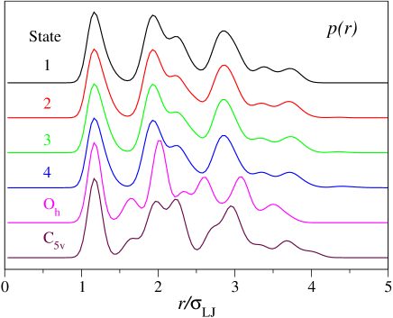
Figure 4: Radial pair correlation functions $p(r)$ for the six FC-VGW states from Table 1. For the liquid-like states 1-4 the radial distributions are nearly identical.

In the context of the VGW approach, we found it sufficient and convenient to characterize the structure of a stationary state by its radial pair correlation function,

$$p(r):=\sum_{i>j}\frac{\langle q_{0};\tau|\delta(|r_{ij}|-r)|q_{0};\tau\rangle}{\langle q_{0};\tau|q_{0};\tau\rangle},$$ (20)

which is computable with little numerical effort Neon13 . The use of angular-dependent distribution functions may be more appropriate but is more complicated. In Fig. 4 we present $p(r)$ for the six stationary states from Table 1. Quite interestingly, for the liquid-like states 1-4, they are nearly identical. Moreover, most stationary VGW states found in our calculations had the radial distribution very similar to that of state 1, while only a few states had $p(r)$ similar to that of the icosahedral state ($C_{5v}$). No state with octahedral-like order was ever found.

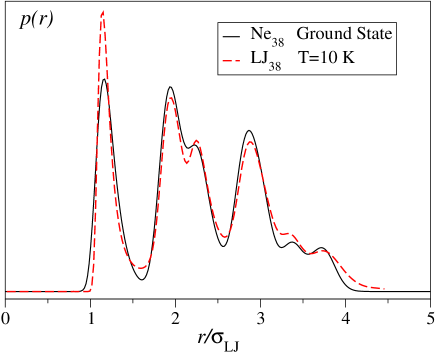
Figure 5: The radial pair correlation function $p(r)$ for the ground state of $\mathrm{Ne}_{38}$ and that for the classical $\mathrm{LJ}_{38}$ cluster at $T=10$ K. The latter was scaled according to $p_{\rm scaled}(r)=\alpha p(r/\alpha)$ with $\alpha=0.97$ before plotting.

Perhaps a more convincing proof that the ground state of the quantum $\mathrm{Ne}_{38}$ cluster corresponds to a disordered, liquid-like state is the similarity between the radial distribution function of the quantum ground state and the radial distribution function of the classical $\mathrm{LJ}_{38}$ system at the temperature of $10~{}\mathrm{K}$ (see Fig. 5). The latter system is in liquid phase at $10~{}\mathrm{K}$, as apparent from Fig. 2. (Note that the classical radial correlation function was scaled using $p_{\rm scaled}(r)=\alpha p(r/\alpha)$ with $\alpha=0.97$ in order to take into account the inflation of the quantum system relative to the classical one.)

Because it is more flexible than the SP-VGW, the FC-VGW provides a better approximation for the ground state. While both approximations fail to correctly describe the low energy rotation of the cluster, the SP-VGW does not correctly describe the translational motion. These are the obvious sources of the systematic errors in the energy estimates using the Gaussian approximations. We found empirically that, for the FC-VGW, the main contribution to the error in the mean energy estimate E(T) is proportional to the system size $N$ and is nearly temperature-independent. This explains the surprising agreement for the heat capacity estimate $C_{v}(T):=\partial E(T)/\partial T$ computed at the level of the FC-VGW theory and well-converged PIMC results for the Ne₁₃ cluster Neon13 .

Qualitatively, the status of the SP-VGW based approximation is similar to that for the FC-VGW. However, the systematic error is about twice as big. From Tables 1 and 2, we can see that the energies (per particle) of the selected states estimated by SP-VGW are shifted by approximately 3 $k_{\rm B}$K per atom relative to those estimated by the more accurate FC-VGW technique, independent of the state. Also the SP-VGW gives different energy ordering for states 1, 2 and 3.

In order to verify the VGW results, we have also performed low temperature PIMC calculations using the initial conditions defined by the centroids of the corresponding Gaussians. The simulation is explained in the last paragraph of Section III and it has been conducted at the temperature of $T=1.78$ K. For each of the six cases reported in Table 1, during the course of the MC simulation, the path was always localized in the same small region of the configuration space where it started. This was checked by a quenching procedure which consisted in finding the classical potential minimum nearest to the quantum path (see Table 1). Note that each of the two lowest quantum states (1 and 2) have resulted in two close minima upon quenching. For each of these two states we checked that the VGW gave the same stationary state when propagated from either of the two classical minima. For state 1 the two classical minima are separated by a barrier with height by an order of magnitude smaller than the estimated value of the ZPE, implying that the ground state must be delocalized over a region including at least these two classical minima.

For the simulation temperature (1.78 K) utilized in the PIMC calculations, the state energies are systematically overestimated by about $0.1$ k_BK per atom. The latter error estimate was obtained by investigating the temperature dependence of the corresponding VGW energies.

The discrepancy between the PIMC and the FC-VGW energies is about 3 $k_{\rm B}$K, independent of the state, which supports our previous observation. This is clearly seen in Table 2, which gives the energies with respect to the ground state energy. That is, after the subtraction of the systematic errors, the agreement between the two methods is quite remarkable.

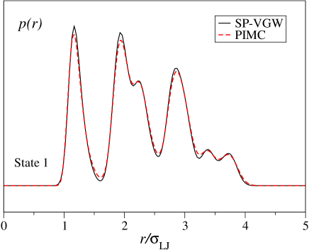
Figure 6: The radial pair correlation function of the ground state computed by the FC-VGW and the PIMC methods.

In Fig. 6, we compare the radial pair correlation function for state 1 computed by FC-VGW and PIMC. The good agreement between the two results is another demonstration of the reliability of the FC-VGW method.

VI Heat capacities for the quantum Ne₃₈ Lennard-Jones cluster.

For the heat capacity calculations, we employed the less expensive SP-VGW version of the method, which proved to be sufficiently accurate for this purpose Neon13 . As for the classical simulations, the same confining radius of $R_{c}=3.612\sigma_{\rm LJ}$ is used here.

The results for the entire temperature range (1 K $<T<$ 11.5 K) were obtained within a single MC calculation using $T_{\rm MC}=11.5$ K. The standard Metropolis algorithm was implemented using 25% acceptance rate. Every new Gaussian was sampled by randomly shifting one of the atoms. Then this Gaussian, with the initial conditions defined by Eq. 11 at the initial inverse temperature $\tau_{0}=10^{-4}(k_{\rm B}\rm K)^{-1}$, was propagated up to $\tau=1/2k_{\rm B}T_{\rm MC}$, where its acceptance probability was evaluated and realized according to the Metropolis procedure. Once a Gaussian wavepacket is accepted, it is further propagated up to $\tau=0.5(k_{\rm B}\rm K)^{-1}$, in order to cover the remaining temperature range of interest. The total number of accepted Gaussian wavepackets was $3\times 10^{7}$. The calculations were performed on a 12-processor 1.4 GHz Opteron cluster. The cpu time on a single processor was about 0.5 seconds per accepted Gaussian wavepacket.

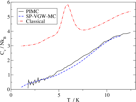
Figure 7: Heat capacity for the Ne₃₈ Lennard-Jones cluster computed by two different methods. The result for a classical LJ₃₈ cluster is also shown.

The results for both the SP-VGW and PIMC simulations are shown in Figs. 7 and 8. The results for the latter technique are for the interval $[1.78~{}\mathrm{K},12.46~{}\mathrm{K}]$. At $1~{}\mathrm{K}$, the PIMC technique would have required $512$ path variables and more parallel tempering replicas, which we found rather expensive. The statistical errors for the SP-VGW heat capacity were estimated by breaking the whole calculation into two independent pieces consisting of $1.5\times 10^{7}$ MC steps each (see Fig. 8). Given the extreme complexity of the system, the agreement between the two methods is remarkable. Within statistical errors, one may safely conclude that there are no peaks in the caloric curve of the quantum Ne₃₈ Lennard-Jones cluster for the temperature regime considered. Less clear is whether or not there is a shoulder in the low-temperature portion of the heat capacity curve, shoulder that could be assigned to a transition between configurations 1 and 2.

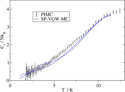
Figure 8: Error bars for the results shown in Fig. 7. The two solid curves correspond to two independent VGW-MC calculations each using $1.5\times 10^{7}$ MC steps.

Finally, in Fig. 9, we show the radial pair correlation functions computed by PIMC for several temperatures, including that of state 1. As opposed to what happens for the classical simulation (see Fig. 3), the quantum results clearly indicate that there is no abrupt change in the equilibrium structure of Ne₃₈, for the entire temperature interval considered. For all temperatures considered, the quantum canonical ensemble for $\mathrm{Ne}_{38}$ consists mainly of configurations that Neirotti and coworkers Neirotti_Ne38 have identified as pertaining to the liquid phase.

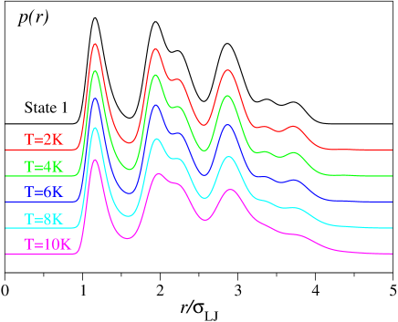
Figure 9: The radial pair correlation functions computed by the PIMC at various temperatures. The result for the ground state is also shown.

VII Summary and conclusions

We have investigated several thermodynamic and structural properties of the quantum $\mathrm{Ne}_{38}$ cluster using two Monte Carlo techniques: the variational Gaussian-wavepacket method and the path integral method. As demonstrated by the results presented in the preceding sections, the effective topology of the potential energy surface is strongly affected by the quantum effects. For example, the highly-symmetric octahedral and icosahedral configurations that dominate the low-temperature classical canonical ensemble have negligible contribution to the quantum canonical ensemble. The $\mathrm{Ne}_{38}$ cluster is found to be essentially liquified for all temperatures investigated.

The configurations of lowest quantum energy are delocalized over basins associated with at least two classical local minima. This strong delocalization explains why the Harmonic Approximation does not provide adequate estimates for quantum energies. Moreover, perturbation theory based on inclusion of the unharmonic terms would not improve the results of the latter. For these techniques to be even applicable, the quantum states must be well localized around one classical minimum. The strong delocalization is actually expected, given that $38$ is not a magic number. The incomplete layer over the icosahedral core has high mobility and is strongly affected by the quantum effects. As previous simulations for $N=7,13$ have shown, for magic numbers, the quantum effects, although strong, do not essentially change the shape of the heat capacity curve.

An important conclusion of the present investigation is that the quantum simulation techniques have matured enough that rather complex system may be directly investigated. For the path integral technique utilized, further work is necessary in order to provide better estimates or criteria relating the quantum effects to the number of path variables. Such criteria are important, for example, in the context of parallel tempering. The present simulation has utilized a number of $256$ path variables for the whole interval $[1.78~{}\mathrm{K},12.46~{}\mathrm{K}]$. However, a number of $32$ path variables would have been enough for the largest temperatures. The computational resources saved would find a better utilization in increasing the number of Monte Carlo steps for the higher temperatures (at least by a factor of $8$). Criteria that could ensure a smooth as well as adequate transition of the number of path variables with the temperature are highly desirable.

The variational Gaussian wavepacket technique has demonstrated again its reliability, providing results consistent with those obtained by path integral simulations. Still, further work is necessary in order to improve the convergence of the underlying Monte Carlo simulation. Thus, the method must be adapted for use with parallel tempering simulation techniques. Such an improvement would avoid having to rely on the configurations generated by a single-temperature Monte Carlo walk.

It is worth mentioning that the two quantum simulation techniques can be used together as complementary tools, each having its particular strengths. The path integral technique has the advantage of being essentially exact, provided enough computational resources are available. In the form it has been implemented in the present application, it can be applied to the most general, many-body potentials, for which the requirement of having analytic expressions for the Gaussian integrals may not be practical. The VGW technique is generally faster and provides results that are more amenable to interpretation. It has also the advantage that it can be more easily adapted for the study of quantum-dynamical properties, if imaginary-time propagation of wavepackets is followed by real-time propagation. As illustrated in the present application, the VGW technique can be used to further quench high-temperature path integral configurations to temperatures so low that a direct path integral simulation is not feasible.