Comment on “Scientific collaboration networks. II. Shortest paths, weighted networks, and centrality”

Abstract

In this comment, we investigate a common used algorithm proposed by Newman [M. E. J. Newman, Phys. Rev. E 64, 016132(2001)] to calculate the betweenness centrality for all vertices. The inaccurateness of Newman’s algorithm is pointed out and a corrected algorithm, also with O($MN$) time complexity, is given. In addition, the comparison of calculating results for these two algorithm aiming the protein interaction network of Yeast is shown.

Betweenness centrality, also called load or betweenness for simplicity, is a quite useful measure in the network analysis. This conception is firstly proposed by AnthonisseAnthonisse1971 and FreemanFreeman1977 and introduced to physics community by NewmanNewman2001 . The betweenness of a node $v$ is defined as

$$B(v):=\sum_{s\neq t,s\neq v}\frac{\sigma_{st}(v)}{\sigma_{st}},$$ (1)

where $\sigma_{st}(v)$ is the number of shortest paths going from $s$ to $t$ passing through $v$ and $\sigma_{st}$ is the total number of shortest paths going from $s$ to $t$. The end points of each path is counted as part of the pathNewman2001 . Newman proposed a very fast algorithm taking only O($MN$) time to calculate the betweenness of all verticesNewman2001 , where $M$ and $N$ denote the number of edges and vertices, respectively. The whole algorithm processes are as follows.

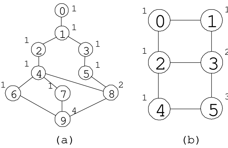
Figure 1: The two examples used to illuminate the difference between Newman’s and the corrected algorithms. (a) The copy from Ref. [2], also bas been used as a sketch map for Newman’s algorithm. (b) The minimal network that can illuminate the difference. The hollow circles represent the vertices and the solid lines represent the edges. Each vertex is marked with a natural number inside the corresponding circle, and the number beside each vertex $v$ is $\sigma_{0v}$.

(1) Calculate the distance from a vertex $s$ to every other vertex by using breadth-first search.

(2) A variable $b_{v}^{s}$, taking the initial value 1, is assigned to each vertex $v$.

(3) Going through the vertices $v$ in order of their distance from $s$, starting from the farthest, the value of $b_{v}^{s}$ is added to corresponding variable on the predecessor vertex of $v$. If $v$ has more than one predecessor, then $b_{v}^{s}$ is divided equally between them.

(4) Go through all vertices in this fashion and records the value $b_{v}^{s}$ for each $v$. Repeat the entire calculation for every vertex $s$, the betweenness for each vertex $v$ is obtained as

$$B(v)=\sum_{s}b_{v}^{s}.$$ (2)

Table 1: Calculation results of figure 1(a)

Vertices	0	1	2	3	4	5	6	7	8	9
Newman’s	9	34$\frac{5}{6}$	28$\frac{1}{6}$	22$\frac{1}{2}$	29$\frac{1}{3}$	21$\frac{2}{3}$	14$\frac{1}{4}$	14$\frac{1}{4}$	21$\frac{5}{6}$	24$\frac{1}{6}$
Corrected	9	34$\frac{1}{3}$	28$\frac{1}{3}$	21$\frac{2}{3}$	30	21	14$\frac{2}{3}$	14$\frac{2}{3}$	21$\frac{2}{3}$	24

Table 2: Calculation results of figure 1(b)

Vertices	0	1	2	3	4	5
Newman’s	6$\frac{3}{4}$	6$\frac{3}{4}$	11$\frac{1}{2}$	11$\frac{1}{2}$	6$\frac{3}{4}$	6$\frac{3}{4}$
Corrected	6$\frac{2}{3}$	6$\frac{2}{3}$	11$\frac{2}{3}$	11$\frac{2}{3}$	6$\frac{2}{3}$	6$\frac{2}{3}$

Since to a vertex $v$’s betweenness $B(v)$, the contributions of its predecessors are not equal, it is not proper to divide $b_{v}^{s}$ equally between them. Clearly, if the vertex $v$ has $n$ predecessors labelled as $u_{1},u_{2},\cdots,u_{n}$ and $\sigma_{sv}$ different shortest paths to vertex $s$, then we have

$$\sigma_{sv}=\sum^{n}_{i=1}\sigma_{su_{i}}.$$ (3)

The different shortest paths from $s$ to $v$ are divided into $n$ sets $G_{1},G_{2},\cdots,G_{n}$. The number of elements in $G_{i}$, that is also the number of different shortest paths from $s$ to $u_{i}$ , gives expression to the contribution of the predecessor $u_{i}$ to $v$’s betweenness. Therefore, the vertex $v$’s betweenness, induced by the given source $s$, should be divided proportionally to $\sigma_{su_{i}}$ rather than equally between its predecessors. The corrected algorithm is as follows.

(1) Calculate the distance from a vertex $s$ to every other vertex by using breadth-first search, taking time O($M$).

(2) Calculate the number of shortest paths from vertex $s$ to every other vertex by using dynamic programmingBellman1962 , taking time O($M$) too. The processes are as follows. (2.1) Assign $\sigma_{ss}=0$. (2.2) If all the vertices of distance $d(d\geq 0)$ is assigned (Note that the distance from $s$ to $s$ is zero), then for each vertex $v$ whose distance is $d+1$, assign $\sigma_{sv}=\sum_{u}\sigma_{su}$ where $u$ runs over all $v$’s predecessors. (2.3) Repeat from step (2.1) until there are no unassigned vertices left.

(3) A variable $\beta_{v}^{s}$, taking the initial value 1, is assigned to each vertex $v$.

(4) Going through the vertices $v$ in order of their distance from $s$, starting from the farthest, the value of $\beta_{v}^{s}$ is added to corresponding variable on the predecessor vertex of $v$. If $v$ has more than one predecessor $u_{1},u_{2},\cdots,u_{n}$, $\beta_{v}^{s}$ is multiplied by $\sigma_{su_{i}}/\sigma_{sv}$ and then added to $\sigma_{su_{i}}$.

(5) Go through all vertices in this fashion and records the value $\beta_{v}^{s}$ for each $v$. Repeat the entire calculation for every vertex $s$, the betweenness for each vertex $v$ is obtained as

$$B(v)=\sum_{s}\beta_{v}^{s}.$$ (4)

Clearly, the time complexity of the corrected algorithm is O($MN$) too. Besides, one should pay attention to a more universal algorithm proposed by BrandesBrandes2001 , which can be used to calculate all kinds of centrality based on shortest-paths counting for both unweighted and weighted networks.

These two algorithms, Newman’s and the corrected one, will give the same result if the network has a tree structure. However, when the loops appear in the networks, the diversity between them can be observed. Figure (1) exhibits two examples, the first one is copied from the Ref. [2], and the second is the minimal network that can illuminate the difference between Newman’s and the corrected algorithms. The comparisons between these two algorithms are shown in table (1) and (2). The two algorithms produce different results even for networks of very few vertices.

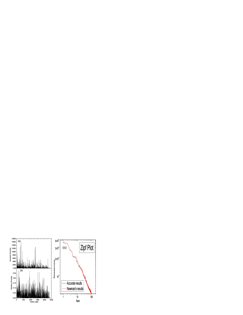
Figure 2: The comparisons between Newman’s and the corrected algorithms on the protein interaction network of Yeast. (a) and (b) shown the absolute diversity and relative diversity between Newman’s and the accurate results, respectively. (c) is the Zipf plot of the 100 vertices with highest betweenness.

In addition, we compare with the performances of these two algorithms on the protein interaction network of YeastJeong2001 . This network has 2617 vertices, but only its maximal component containing 2375 vertices is taken into account. Figure 2(a) and 2(b) report the absolute diversity and relative diversity between Newman’s and the accurate (obtained from the corrected algorithm) results, respectively. The departure is distinct and can not be neglected. Fortunately, the statistical features may be similar. Although the details of the Zipf plotZipf1949 of the top-100 vertices are not the same, both the two curves obey power-law form with almost the same exponent. We also have checked that the scaling lawGoh2001 ; Goh2002 of betweenness distribution in Barabási-Albert networksBarabasi1999 is kept, while the power-law exponents are slightly changed.

The measure of betweenness is now widely used to detect communities/modules structuresGirvan2002 ; Newman2004 and to analysis dynamics upon networks. Since the statistical characters of betweenness distributions obtained by Newman’s and the corrected algorithm are almost the same, some researchers may have found the difference between these two algorithm but have not paid attention to it. However, many previous works have demonstrated that a few nodes’ betweennesses rather than the overall betweenness distribution, may sometimes, determine the key features of dynamic behaviors on networks. Examples are numerous: these include the network trafficsGuimera2002 ; Zhao2005 ; Yan2005 , the synchronizationNishikawa2003 ; Hong2004 ; ZhaoM2005 , the cascading dynamicsMotter2004 , and so on. In figure 2(b), one can find that for many nodes the relative diversities betweenness those two algorithms exceed $10\%$, and even nearly $30\%$ for a few nodes. Therefore, the difference can not be neglected especially in analyzing the networks dynamics.

Although Newman’s algorithm does not agree with the definition of betweennessNewman2001 , it may be more practical especially for the large-scale communication systems wherein the routers do not know how many shortest paths there are to the destination. Even if they can save the information of all the successors’ weights, to implement the biased choices may bring additional costs in economy and technique. Hence just to choose with equal probability at each branch point may be more natural, which is in accordance with Newman’s algorithm.

References

- (1) J. M. Anthonisse, Technical Report BN 9/71, Stichting Mathematisch Centrum, Amsterdam.
- (2) L. C. Freeman, Sociometry 40, 35 (1977).
- (3) M. E. J. Newman, Phys. Rev. E 64, 016132 (2001).
- (4) R. E. Bellman, and S. E. Dreyfus, Applied Dynamic Programming (Princeton University Press, New Jersy, 1962).
- (5) U. Brandes, Journal of Mathematical Sociology 25, 163(2001).
- (6) H. Jeong, S. Mason, A. -L. Barabási, and Z. N. Oltvai, Nature 411, 41 (2001).
- (7) G. K. Zipf, Human Behavior and the Principal of Least Effort (Addison-Wesley, Cambridge, MA, 1949).
- (8) K. -I. Goh, B. Kahng, and D. Kim, Phys. Rev. Lett. 87, 278701 (2001).
- (9) K. -I. Goh, E. Oh, H. Jeong, B. Kahng, and D. Kim, Proc. Natl. Acad. Sci. USA 99, 12583 (2002).
- (10) A. -L. Barabási, and R. Albert, Science 286, 509 (1999).
- (11) M. Girvan, and M. E. J. Newman, Proc. Natl. Acad. Sci. U.S.A. 99, 7821 (2002).
- (12) M. E. J. Newman, and M. Girvan, Phys. Rev. E 69, 026113(2004).
- (13) R. Guimerá, A. Díaz-Guilera, F. Vega-Redondo, A. Cabrales, and A. Arenas, Phys. Rev. Lett. 89, 248701 (2002).
- (14) L. Zhao, Y.-C. Lai, K. Park, and N. Ye, Phys. Rev. E 71, 026125 (2005).
- (15) G. Yan, T. Zhou, B. Hu, Z. -Q. Fu, and B. -H. Wang, arXiv: cond-mat/0505366.
- (16) T. Nishikawa, A. E. Motter, Y. -C. Lai, and F. C. Hoppensteadt, Phys. Rev. Lett. 91 014101 (2003).
- (17) H. Hong, B. J. Kim, M. Y. Choi, and H. Park, Phys. Rev. E 69, 067105(2004).
- (18) M. Zhao, T. Zhou, B. -H. Wang, and W. -X. Wang, Phys. Rev. E 72, 057102(2005).
- (19) A. E. Motter, Phys. Rev. Lett. 93, 098701 (2004).