Description of ⁴He tetramer bound and scattering states

Abstract

Faddeev-Yakubovski equations are solved numerically for ⁴He tetramer and trimer states using realistic helium-helium interaction models. We describe the properties of ground and excited states, and we discuss with a special emphasis the ⁴He-⁴He₃ low energy scattering.

I Introduction

Helium atom is one of the simplest few-body systems. Nowadays, its structure can be described theoretically with an accuracy better than the spectroscopy one Atoms . In spite of this simplicity, the compounds of Helium atoms display a series of unique microscopic and macroscopic physical phenomena.

The closed shell electronic structure, as well as the compactness of the Helium atom, makes it the most chemically inert noble gas. Nevertheless, the very weak van der Waals attraction between two distant He atoms is responsible for the fact that at very low temperatures, both bosonic ⁴He and fermionic ³He liquify. In addition, the extreme weakness of the He-He interaction is decisive in explaining why liquid Helium is the only known superfluid.

As much exciting is the physics of the atomic Helium nanoscopic structures (He multimers). Recent inspiring experiments Spuch ; Toennies have demonstrated the existence of bound diatomic ⁴He systems (dimers) - the ground state with the weakest binding energy of all naturally existing diatomic molecules. Moreover, diffraction experiment projecting a molecular beam of small He clusters on nanostructured transmission gratings, allowed a direct measurement of the dimer average bond length value $<R>=52\pm 4$ $\AA$. Such a large bond, compared to the effective range of the He-He potential, enables one to estimate its binding energy $E\approx\frac{\hbar^{2}<R>^{2}}{4m}=1.1+0.3/-0.2$ mK, as well as the ⁴He-⁴He scattering length $a_{0}=104+8/-18$ $\AA$.

The extreme weakness of the ⁴He dimer binding energy requires a precise theoretical description of the ab initio He-He potential, which results from subtracting the huge energies of separated atoms. Nevertheless, several very accurate theoretical models Aziz ; Aziz1 ; Aziz2 ; Aziz3 ; Tang_toennies ; Aziz4 were recently constructed, predicting Helium properties in full agreement with experiments. These effective He-He potentials are dominated by the strong repulsion (hard-core) at distances $R_{He-He}\lesssim 2$ $\AA$, where the two He atoms are ”overlapping”. At larger He-He distances, the weak van-der-Waals attraction takes over, creating a shallow attractive pocket with a maximal depth of $V_{0}\approx 10.9$ K, centered at $R_{He-He}\approx 3\AA$. The strong repulsion of the He-He potential at short distance, allows to treat accurately atomic He systems without having to take into account the internal structure of single He atoms.

The physics of small He clusters is an outstanding laboratory for testing different quantum mechanical phenomena. The bound state of ⁴He dimer, at practically zero energy, suggests the possibility of observing an Efimov-like state in the triatomic compound Efimov . The existence of this ⁴He dimer bound state very close to threshold, is also responsible for a resonant ⁴He-⁴He S-wave scattering length $a_{0}\approx$104 $\AA$, which is more than 30 times larger than the typical length scale given by the Van der Waals interaction $l\sim 3\AA$. The small He clusters low energy scattering observables should therefore be little sensitive to the details of He-He interaction and should thus exhibit some universal behavior. This sharp separation of different scales can be exploited, making He multimers a perfect testground for Effective Field Theory (EFT) approaches  EFT_intro1 ; EFT_intro2 ; Hammer ; Platter .

We present in this work a rigorous theoretical study of the smallest ⁴He clusters. There exist in the literature a large number of theoretical calculations on triatomic ⁴He (trimer) Gloeckle ; Sandhas ; Barletta . However the four-atomic ⁴He system (tetramer), being by an order of magnitude more complex in its numerical treatment, remains practically unexplored. Our study tries to fill up this gap, by providing original calculations for tetramer bound and scattering states. In addition, some existing ambiguities in triatomic ⁴He calculations Roudnev_ss are discussed.

To describe ⁴He tetramer, Faddeev-Yakubovski (FY) equations in configuration space are solved. In some cases, this method may be cumbersome and numerically expensive. It constitutes nevertheless a very general and mathematically rigorous tool, with the big advantage over many other techniques, that it enables a systematic treatment of bound and continuum states.

The paper is structured as follows: in section II we present the theoretical framework used; in section III we highlight our ⁴He trimer results. Section IV deals with four-atomic helium systems and in section V, we discuss the possible existence of the rotational states in three-atomic and four-atomic⁴He systems. Section VI concludes this work with the final remarks.

To describe the interaction between the helium atoms, we have used the potential developed by Aziz and Slaman Aziz , popularly referred to as LM2M2 potential. There exists several equivalent interaction models. However, they all have similar structure and quantitatively provide very close results Barletta ; Sandhas_last .

All results presented in this paper are restricted to the bosonic ⁴He isotope; therefore in the following, we omit the mass number 4 and refer to ⁴He as He. All calculations use $\frac{\hbar^{2}}{m}=12.12$ K$\cdot$Ų as the input mass of He atoms.

II Theoretical framework

II.1 Faddeev-Yakubovski equations

The Schrödinger equation is the paradigm of non-relativistic quantum mechanics. However this equation is not able to separate different rearrangement channels in the asymptote of multiparticle wave function (w.f.). Thus it does not provide explicitly a way to implement the physical boundary conditions for scattering w.f., which are necessary to obtain a unique solution. Faddeev Faddeev have succeeded to show that these equations can be reformulated by introducing some additional physical constraints, what leads to mathematically rigorous and unique solution of the three-body scattering problem. Faddeev’s pioneering work was followed by Yakubovsky. In Yakubovski , the systematic generalization of Faddeev equations for any number of particles was presented.

One should mention that Schrödinger equation may still be applied when solving few-particle bound state problem. However then one must deal directly with total systems w.f., which is fully (anti)symmetric and has quite complicated structure. Exploiting the knowledge of systems symmetry one often tries to decompose this w.f. into only partially (anti)symmetrized components, which had simpler structure and are more tractable numerically. One practical way is to decompose systems w.f. into so called FY components. Then FY equations often have obvious advantage over Schrödinger one, since it deals directly only with FY components by avoiding construction of full system wave function.

In that follows, we describe only four-particle FY equations; three-particle Faddeev equations are self-contained in four-particle ones.

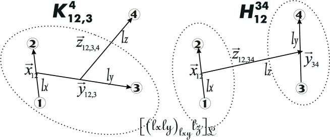
Figure 1: Faddeev-Yakubovsky components $K$ and $H$. Asymptotically, as $z\rightarrow\infty$, components $K$ describe 3+1 particle channels, whereas components $H$ contain asymptotic states of 2+2 channels.

The calculations presented in this work were performed using the framework of differential FY equations developed by S.P. Merkuriev and S.L. Yakovlev Yakovlev ; Merkuriev . The major step in these equations is the representation of the systems w.f. as a sum of 18 components: 12 of type K, describing the asymptotic behavior of different 3+1 particle channels, and 6 of type H, describing the systems decomposition into two clusters of two particles:

$$\Psi=\sum\limits_{i<j}K_{ij,k}^{l}+\sum\limits_{i<j,k<l}H_{ij,kl}.$$ (1)

Here $\left(ijkl\right)$ indicates cyclic permutation of particle indices $(1234)$. These FY components are coupled by 18 FY equations. Since all particles are identical, several straightforward symmetry relations can be established between different FY components. Using these relations, the number of independent FY equations and components reduces to two:

$$\left(E-\hat{H}_{0}-\hat{V}\right)K_{12,3}^{4} = \hat{V}(P^{+}+P^{-})\left[(1+\varepsilon P_{34})K_{12,3}^{4}+H_{12,34}\right]\vskip 3.0pt plus 1.0pt minus 1.0pt$$ (2)

$$\left(E-\hat{H}_{0}-\hat{V}\right)H_{12,34} = \hat{V}\tilde{P}\left[(1+\varepsilon P_{34})K_{12,3}^{4}+H_{12,34}\right].$$

Here $P^{+}=P_{12}P_{23}$, $P^{-}=P_{23}P_{12}$ and $\tilde{P}=P_{13}P_{24}$ are particle permutation operators. $\hat{H}_{0}$ is the kinetic energy operator of the system and $\hat{V}$ is the potential energy operator for the particle pair (12). The coefficient $\varepsilon$ is a Pauli factor: $\varepsilon=1$ for bosonic systems and $\varepsilon=-1$ for systems of identical fermions.

By applying combination of permutation operators to the FY components of Eq. (1), one can express the w.f. of the system by means of two non-reducible FY components:

$$\Psi=\left[1+(1+P^{+}+P^{-})\varepsilon P_{34}\right](1+P^{+}+P^{-})K_{12,3}^{4}+(1+P^{+}+P^{-})(1+\tilde{P})H_{12,34}$$ (3)

It is convenient to treat Eq. (2) using relative reduced coordinates. These coordinates are proportional to well known Jacobi coordinates, which are simply scaled by the appropriate mass factors. We use two different sets of relative reduced coordinates, defined as follows:

$$\overrightarrow{x_{ij}}$$

(4)

for $K-$type FY components. $m_{i}$ and $\overrightarrow{r}_{i}$ are respectively the $i$-th particle mass and position vector. To describe $H-$type components, another set of coordinates is more appropriate:

$$\overrightarrow{x_{ij}}$$

(5)

Using these coordinates, the kinetic energy operator is expressed as a simple sum of Laplace operators:

$$H_{0}=-\frac{\hbar^{2}}{2m}\Delta_{R}-\frac{\hbar^{2}}{m}\left(\Delta_{x}+\Delta_{y}+\Delta_{z}\right).$$ (6)

Another big advantage of these coordinate sets is the fact that the degrees of freedom due to the center of mass motion are separated.

The dimension of the problem can be further reduced by using the fact that an isolated system conserves its total angular momentum $\mathcal{J}$ and one of its projections $\mathcal{J}_{z}$. We deal with systems of bosonic He atoms in their ground state, which have a total spin equal to zero. In this case, the system w.f. is independent of the spin and the orbital angular momentum is conserved separately. Using this fact, we expand FY components on a partial-wave basis (PWB) of orbital angular momentum and, omitting the spin:

(9)

In this basis, the kinetic energy operator reads:

$$\hat{H}_{0}=\frac{\hbar^{2}}{m}\left[-\partial_{x}^{2}-\partial_{y}^{2}-\partial_{z}^{2}+\frac{l_{x}(l_{x}+1)}{x^{2}}+\frac{l_{y}(l_{y}+1)}{y^{2}}+\frac{l_{z}(l_{z}+1)}{z^{2}}\right].$$

In Eq. (9), we have introduced the so called FY amplitudes $\mathcal{F}_{\alpha}^{K}(x,y,z)$ and $\mathcal{F}_{\alpha}^{H}(x,y,z)$, which are continuous functions in radial variables $x$,$y$ and $z$. The symmetry properties of the w.f. with respect to the exchange of two He atoms impose additional constraints. One should have amplitudes only with an even value of the angular momentum $l_{x}$, whether these amplitudes are derived from $K$ or $H$ FY components.

In addition, for $H-$type amplitudes $\mathcal{F}_{\alpha}^{H}(x,y,z)$, the angular momentum $l_{y}$ should be even as well. The total parity of the system $\Pi$ is given by $\left(-\right)^{l_{x}+l_{y}+l_{z}}$ independently of the coupling scheme ($K$ or $H$) used.

By projecting each of the Eq. (2) to the PWB of Eq. (9), a system of coupled integro-differential equations is obtained. In general, PWB is infinite and one obtains thus an infinite number of coupled equations. This obliges us, when solving these equations numerically, to make additional truncations by considering only the most relevant amplitudes, namely those which have the smoothest angular dependency (small partial angular momentum values $l_{x},l_{y}$ and $l_{z}$).

II.2 Boundary conditions

Equations (2) are not complete: they should be supplemented with the appropriate boundary conditions for FY components. It is usual to write boundary conditions in the Dirichlet form, which at the origin should mean vanishing FY components. However, the existence of a large strong repulsion region (hard-core) corresponding to the inner part of He-He potential brings additional complications. The relevant matrix elements from the physical interaction region (shallow attractive well) fade away in front of the huge repulsive hard-core terms, thus resulting in severe numerical instabilities.

However, such a strong repulsion at the origin simply indicates that two He atoms cannot get arbitrarily close to each other: for a repulsive region of characteristic size $r_{h}$, the probability that two particles get closer to each other at a certain distance $r=c<r_{h}$ will be vanishingly small. It means that the w.f. of the system vanishes in part of a four-particle space, inside six multidimensional surfaces $r_{ij}=c,$ where $r_{ij}$ is the distance between particle $i$ and $j$. The most straightforward way to improve numerical stability would be to avoid calculating the solution in at least part of the strong repulsion region, and to impose by hand to the wave function to be equal to zero in this region. Nevertheless, due to the complex geometry of this domain in the nine-dimensional space of particle relative coordinates, this method is not easy to put in practice.

A nice way to overcome this difficulty was proposed by Motovilov and Merkuriev Motov . The authors showed that an infinitely repulsive interaction at $r_{ij}\leqslant c$, generates boundary conditions for the FY components which can be ensured by setting:

$$\begin{tabular}[]{l}$\left(E-\hat{H}_{0}-\hat{V}\right)K_{12,3}^{4}=0\vskip 3.0pt plus 1.0pt minus 1.0pt$\\ $\left(E-\hat{H}_{0}-\hat{V}\right)H_{12,34}=0$\end{tabular}\text{ for }x<c$$ (12)

and

$$\begin{tabular}[]{l}$K_{12,3}^{4}+(P^{+}+P^{-})\left[(1+\varepsilon P_{34})K_{12,3}^{4}+H_{12,34}\right]=0$\\ $H_{12,34}+\tilde{P}\left[(1+\varepsilon P_{34})K_{12,3}^{4}+H_{12,34}\right]=0$\end{tabular}\text{ for }x=c$$ (15)

In addition, FY components asymptotic behavior should be conditioned as well. For the bound state problem, the w.f. of the system is compact, therefore the regularity conditions can be completed by forcing the amplitudes $\mathcal{F}_{\alpha}^{K(H)}$ to vanish at the borders of the hypercube $\left[0,X_{\max}\right]\times\left[0,Y_{\max}\right]\times\left[0,Z_{\max}\right]$, i.e.:

$$\mathcal{F}_{\alpha}^{K(H)}(X_{\max},y,z)=\mathcal{F}_{\alpha}^{K(H)}(x,Y_{\max},z)=\mathcal{F}_{\alpha}^{K(H)}(x,y,Z_{\max})=0$$ (16)

In the case of elastic atom-trimer (1+3) scattering, the asymptotic behavior of the w.f. can be matched by simply imposing at the numerical border $z=Z_{\max}$, the solution of the 3N bound state problem for all the quantum numbers, corresponding to the open channel $\alpha_{a}$. It worths reminding that only $K$-type components contribute in describing 3+1 particle channels:

$$\mathcal{F}_{\alpha_{a}}^{K}(x,y,Z_{\max})=f_{\alpha_{a}}(x,y)$$ (17)

Indeed, below the first inelastic threshold, at large values of $z$, the solution of Eq. (2) factorizes into a He trimer ground state w.f. – being solution of 3N Faddeev equations – and a plane wave propagating in $z$ direction with the momentum $k_{\alpha_{a}}=\sqrt{\frac{m}{\hbar^{2}}\left(E_{cm}-E_{He_{3}}\right)}$. One has:

$$\mathcal{F}_{\alpha_{a}}^{K}(x,y,z)\sim f_{\alpha_{a}}^{K}(x,y)\left[\hat{\jmath}_{l_{z}}(k_{\alpha_{a}}z)+\tan(\delta)\hat{n}_{l_{z}}(k_{\alpha_{a}}z)\right]$$

Here the functions $f_{\alpha_{a}}^{K}(x,y)$ are the Faddeev amplitudes obtained after solving the corresponding He trimer bound state problem, whereas $E_{He_{3}}$ is its ground state energy; $\hat{n}_{l_{z}}(k_{\alpha_{a}}z)$ and $\hat{j}_{l_{z}}(k_{\alpha_{a}}z)$ are regularized Riccati-Bessel functions. Equations (2) in conjunction with the appropriate boundary conditions define the set of equations to be solved. The numerical methods employed will be briefly explained in the next subsection.

Once the integro-differential equations of the scattering problem are solved, one has two different ways to obtain the scattering observables. The easier one is to extract the scattering phases directly from the tail of the solution, by calculating logarithmic derivative ($\frac{\partial_{z}\mathcal{F}_{\alpha_{a}}^{K}(x,y,z)}{\mathcal{F}_{\alpha_{a}}^{K}(x,y,z)}$ ) of the open channel’s $K$ amplitude $\alpha_{a}$ in the asymptotic region:

$$\tan\delta=\frac{k_{\alpha_{a}}\hat{\jmath}_{l}^{\prime}(k_{\alpha_{a}}z)-\frac{\partial_{z}\mathcal{F}_{\alpha_{a}}^{K}(x,y,z)}{\mathcal{F}_{\alpha_{a}}^{K}(x,y,z)}\hat{\jmath}_{l}(k_{\alpha_{a}}z)}{\frac{\partial_{z}\mathcal{F}_{\alpha_{a}}^{K}(x,y,z)}{\mathcal{F}_{\alpha_{a}}^{K}(x,y,z)}\hat{n}_{l}(k_{\alpha_{a}}z)-k_{\alpha_{a}}\hat{n}_{l}^{\prime}(k_{\alpha_{a}}z)}$$ (18)

This result can be independently verified by using an integral representation of the phase shifts

$$k_{\alpha_{a}}\tan\delta=-\frac{m}{\hslash^{2}}\int\Phi_{\alpha_{a}}^{(123)}\hat{\jmath}_{l}(k_{\alpha_{a}}z)(V_{14}+V_{24}+V_{34})\Psi dV.$$ (19)

$\Phi_{\alpha_{a}}^{(123)}$ is the trimer – composed from the He atoms indexed by 1,2 and 3 – ground state w.f. normalized to unity and $\Psi$ is normalized according to:

$$\Psi(\vec{x}_{i},\vec{y}_{i},\vec{z}_{i})=\Phi_{\alpha_{a}}^{(123)}\left(\vec{x},\vec{y}\right)\left[\hat{\jmath}_{l_{z}}(k_{\alpha_{a}}z)+\tan(\delta)\hat{n}_{l_{z}}(k_{\alpha_{a}}z)\right].$$ (20)

Detailed discussions on this subject can be found in Fred_97 ; Thesis .

II.3 Numerical methods

In order to solve the set of integro-differential equations – obtained when projecting Eq. (2) and the appropriate boundary conditions Eq. (12-17) into a partial wave basis – the components $\mathcal{F}_{i}^{\alpha}$ are expanded in terms of piecewise Hermite spline basis:

$$\mathcal{F}_{i}^{\alpha}(x,y,z)=\sum c^{\alpha}_{ijkl}S_{j}(x)S_{k}(y)S_{l}(z).$$

We use piecewise Hermite polynomials as a spline basis. In this way, the integro-differential equations are converted into an equivalent linear algebra problem with unknown spline expansion coefficients to be determined. For bound states, the eigenvalue-eigenvector problem reads:

$$Ax=EBx,$$ (21)

where $A$ and $B$ are square matrices, while $E$ and $x$ are respectively the unknown eigenvalue(s) and its eigenvector(s). In the case of the elastic scattering problem, a system of linear algebra equations is obtained:

$$\left[A-E_{cm}B\right]x=b$$ (22)

where $x$ is a vector of unknown spline expansion coefficients and $b$ is an inhomogeneous term, generated when implementing the boundary conditions Eq. (17). For detailed discussions on the equations and method used to solve large scale linear algebra problems, one can refer to Thesis .

III Trimer scattering and bound states

As mentioned in the introduction, trimer states have been broadly explored in many theoretical works. Hyperspherical, variational and Faddeev techniques were used to calculate accurately bound state energies Barletta ; Sandhas ; Roudnev_bs ; Claude_mers ; Sandhas_last ; Fedorov_mers ; Blume_mers as well as to test different He-He interaction models. Nevertheless, we found useful to consider these states as a first step, before the more ambitious analysis of He tetramer states could be undertaken. Special emphasis will be attributed to He-He₂ scattering calculations, which are less studied and for which some discrepancies were pointed out Roudnev_ss ; Sandhas_last . Some arguments will also be developed in favor of considering the first trimer excitation as an Efimov state.

We present in Table 1 the convergence of the He trimer states as a function of the partial-wave basis size. It contains results for the ground ($B_{3}$) and first excited ($B_{3}^{*}$) state binding energies as well as for the He-He₂ scattering length ($a_{0}^{(1+2)}$). The basis truncations were made by limiting partial angular momentum values, applying selection criteria $l_{x}=l_{y}\leq l_{max}$. One can remark that the convergence is monotonic and quite similar for the He₃ bound states and for the He-He₂ scattering length calculations. These results demonstrate that in order to ensure five digit accuracy, the partial wave basis must include FY amplitudes with angular momentum values up to 12. However, for reaching a 1% accuracy, $l_{max}=4$ turns out to be enough.

Table 1: Convergence of He trimer calculations obtained when increasing partial wave basis. In the three columns are respectively presented trimer ground (B₃) and excited(B${}^{*}_{3}$) state energies in mK, as well as atom-dimer scattering length ($a_{0}^{(2+1)}$) in $\AA$.

$l_{max}$	B3 (mK)	B${}^{*}_{3}$ (mK)	$a_{0}^{(1+2)}$ (Å)
0	89.01	2.0093	155.39
2	120.67	2.2298	120.95
4	125.48	2.2622	116.37
6	126.20	2.2669	115.72
8	126.34	2.2677	115.61
10	126.37	2.2679	115.58
12	126.39	2.2680	115.56
14	126.39	2.2680	115.56

In Table 2 are summarized some relevant properties of the trimer ground and excited states. Together with their binding energies ($B$) we give some average quantities like kinetic $<T>$ and potential energy $<V>$ values and moments of interparticle distances $x_{ij}$. Our results are in perfect agreement with other existing calculations Blume_mers ; Barletta ; Roudnev_bs ; the most accurate of them have been included in this Table for comparison.

Table 2: Mean values for He trimer ground and excited states. In this table B, T and V indicates respectively binding, mean kinetic and potential energies calculated in mK; $x_{ij}$ stands for interparticle distance.

	Ground state		Excited state
B (mK)	126.39	126.4 Barletta	2.268	2.265 Barletta
$<T>$ (mK)	1658	1660 Barletta	122.1	121.9 Barletta
$<V>$ (mK)	-1785	-1787 Barletta	-124.5	-124.2 Barletta
$\sqrt{<x_{ij}^{2}>}$ ($\AA$)	10.95	10.96 Barletta	104.3	102.7 Roudnev_bs
$<x_{ij}>$ ($\AA$)	9.612	9.636 Barletta	83.53	83.08 Barletta
$<x_{ij}^{-1}>$ ($\AA^{-1}$)	0.135		0.0267
$<x_{ij}^{-2}>$ ($\AA^{-2}$)	0.0230	0.0233 Kornilov	0.00218

The situation is more ambiguous for the He-He₂ scattering length $a_{0}$. Results obtained by Sandhas et al. Sandhas – solving Faddeev equations – and Blume et al. Blume_mers – using hypherspherical harmonics – agreed with each other on a scattering length value $a_{0}=126$ $\AA$. However Roudnev Roudnev_ss , using also Faddeev equations, found a smaller value $a_{0}=115.4\pm 0.1$ $\AA$. It seems that in Sandhas et al. Sandhas calculation a relatively small grid was employed, which did not allow to disentangle the contribution of virtual dimer break-up component in the asymptotic behavior of the wave function. A more recent study Sandhas_last of the same authors provided a value of $a_{0}=115.5\pm 0.5$ $\AA$, in full agreement with Roudnev’s result.

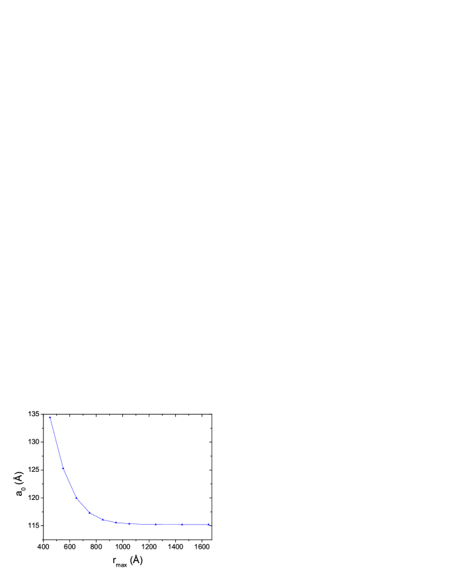
Figure 2: ”(Color online)” Convergence of $He-(He)_{2}$ scattering length obtained when enlarging solution domain of Faddeev equations in $He-(He)_{2}$ separation direction (variable y) with additional discretization points.

Our calculations are also very close to this value. When using a numerical grid limited to $y_{max}=450\;\AA$ we obtain $a_{0}=134\;\AA$, still far from the final result. Note that hyperradial grids employed in Sandhas were limited to $\rho_{\max}=\sqrt{x^{2}+y^{2}}$=460 $\AA$. The results of Table 1 have been obtained using a grid with $y_{max}=950\;\AA$, i.e. He-He₂ distance $r_{max}={\sqrt{3}\over 2}y_{max}=823\;\AA$, which is large enough to reduce the grid-dependent variations to the fourth significant digit. As a function of $r_{max}$, the scattering length varies smoothly (see Figure 2) and converges towards the value $a_{0}(\infty)=115.2$ $\AA$, very close to the one given by Roudnev $a_{0}=115.4\pm 0.1$ $\AA$.

Whether or not the trimer first excitation is an Efimov Efimov state has been an issue of strong polemics Gonsales ; Esry_comm . In fact, when using effective range theory and describing system by zero-range interactions, it is not difficult to show the appearance of an Efimov state. However, the problem becomes complicated in calculations with finite range potentials. Efimov states accumulate according to a logarithmic law

$$N\approx\frac{1}{\pi}\ln\frac{\left|a\right|}{r_{0}}$$

and thus the two body scattering length should be each time increased by a factor $\sim e^{\pi}\approx 23$ (or the dimer binding energy reduced $\sim e^{2\pi}\approx 530$ times) to allow the appearance of an additional Efimov state. To handle this property, the grids employed in calculations should be extremely large and dense, capable on one hand to accommodate extended wave functions, and on the other hand to trace the very weak binding of the third particle to the dimer. Such requirements can not be fulfilled in the calculations with realistic interactions. Thus the basic clue in claiming excited trimer to be an Efimov state is the fact that this state disappears when the interatomic potential is made less attractive Gloeckle ; Esry_init ; Fedorov_non . Actually, if this potential is multiplied by an enhancement factor $\gamma>$ 1 then the following effect is observed: first, the difference between the trimer excited state binding energy ($B_{3}^{*}$) and the dimer one ($B_{2}$) increases with $\gamma$. Then, for larger values of $\gamma$ the difference ($B_{3}^{*}-B_{2}$) monotonously decreases and for $\gamma>$1.2 trimer excited state moves below the dimer threshold and becomes a virtual one.

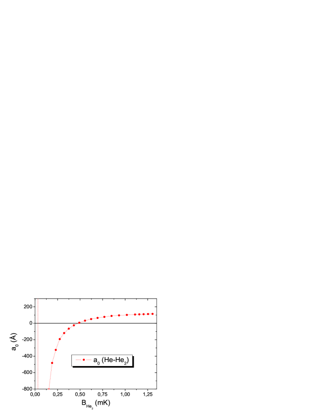
Figure 3: ”(Color online)” The change of the atom-dimer scattering length as a function of the dimer binding energy.

The demonstration of Efimov effect can be accomplished only by showing accumulation of new states when dimer binding energy decreases. Such a demonstration has been given in ref. Kolg_Efim using semi-empirical potential HFD-B Aziz2 . We would like to remark that the formation of new states can be alternatively demonstrated by studying the $\gamma$-dependence of the three-body scattering length, without the necessity of solving the bound state problem. In scattering calculations, the numerical solution of 3-body equations can be reduced to the interaction domain and the wave function extended outside this region using analytical expressions Jaume_dom_meth .

In figure 3 we display the behavior of the He-He₂ scattering lengths, when the He-He potential is multiplied by a scaling factor $\gamma<1$, according to $\tilde{V}=\gamma V$. In this figure, the He-He₂ scattering length is plotted as a function of the fictive dimer binding energy. One can see that, when decreasing $\gamma$ – scattering length decreases. However in absence of Efimov states one should expect them increasing, since reducing $\gamma$, the dimer target becomes larger. Once $\gamma$ is reduced to $\approx 0.990$, the scattering length becomes negative and for values $\gamma\approx 0.979$ it exhibits a singularity going from $a_{0}=-\infty$ to +$\infty$. This singularity corresponds to the appearance of a new trimer bound state (i.e. second excited state in He trimer). This analysis clearly demonstrates that He trimer excited state is an Efimov one. It is worth mentioning that for an enhancement factor $\gamma=0.979$, the He dimer binding energy is only 0.046 $mK$.

IV Tetramer states

The major aim of this article is to provide a comprehensive analysis of the four-atomic He compound (tetramer). The first efforts to describe this system were made already in the late seventies by S. Nakaichi et al. Maeda_var using a variational method. Latter on, variational Montecarlo techniques were used by several authors Blume_mers ; Bresanini ; Lewerenz ; Guardiolla to compute the tetramer ground state. These methods are very powerful in calculating $L^{\Pi}=0^{+}$ bound state properties, but are seldom generalized to describe excited states and are not appropriate for scattering problem.

FY techniques were also used by S. Nakaichi et al. Maeda_FY to calculate the tetramer ground state binding energy and the He-He₃ scattering length. However in order to reduce the – at that time – outmatching numerical costs, some important approximations were made. The He-He potential was restricted to S-wave and written as a one-rank separable expansion and the same expansion was used to represent the FY amplitudes. These approximations led to a tetramer ground state which is underbound by 40% with respect to their own variational result  Maeda_var . A recent attempt to calculate the He tetramer binding energy using S-wave FY equations was done in Roudnev_He4 , although without separable expansion of FY amplitudes.

Table 3: Convergence of the He tetramer calculations obtained when increasing the partial wave basis of Eq. (9). The two columns represent respectively the tetramer ground state binding energy in mK (B₄) the and the atom-trimer scattering length ($a_{0}^{(3+1)}$) in $\AA$.

$\max(lx,ly,lz)$	B4 (mK)	$a_{0}^{(3+1)}$ (Å)
0	348.8	$\approx$-855
2	505.9	190.6
4	548.6	111.6
6	556.0	105.9
8	557.7	103.7

The FY calculations we present here contain no approximation other than the finite basis set used in the partial wave expansion (9). This basis set included amplitudes with internal angular momentum not exceeding a given fixed value $l_{max}$, i.e. fulfilling the condition $max(l_{x},l_{y},l_{z})\leq l_{max}$. The largest basis we have considered has $l_{max}=$8, and consist of 180 FY amplitudes, a number by two order of magnitude larger than in preceding calculations. Note, that the smallest basis, which is often referred to as S-wave approximation, is obtained by fixing $l_{max}=0$ and requires only 2 amplitudes, one of type K and one of type H. The convergence is displayed in Table 3 for the tetramer ground state binding energy and He-He₃ scattering length.

The corresponding FY K-amplitudes are displayed in Figure 4 as a function of the He-He₃ distance $r=\sqrt{2\over 3}z$. One can see the different scales involved in the bound state and zero energy scattering wave function.

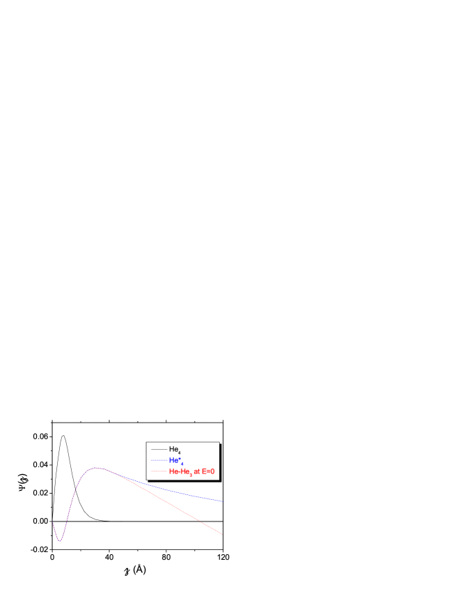
Figure 4: ”(Color online)” Comparison of the functional dependence of K-type FY components in one He atom separation from He₃ core direction. Single, dashed and dot line curves correspond respectively to tetramer ground, excited state and He-He₃ zero energy scattering wave functions.

The convergence of the tetramer calculations is sensibly slower than the one observed for the trimer case (see Table 1). Such a deterioration is due to the complex structure of the involved FY components. Indeed, each He atom pair brings an additional hard-core region; the ensemble of these regions crosses over in the multidimensional configuration space and results into a single domain with non trivial geometry. Inside this multidimensional domain, the total wave function must vanish by cancelling the contributions of the different FY amplitudes, what can be achieved only at the price of increasing its functional complexity.

The convergence of the He-He₃ scattering calculations is also slightly slower than for tetramer ground state. This is a consequence of the scattering wave function, which presents a richer structure than the ground state one, as can be seen in Figure 4. Tetramer ground state has a rather simple geometry: the four He atoms minimize their total energy by forming a tetrahedron. The total energy of the 1+3 scattering state ($E\approx-126$ mK) is considerably larger than the ground state one ($E\approx-558$ mK) and provides more flexibility to each atom. Furthermore, since the scattering length value is much larger than the size of the trimer target, the scattering wave function turns to be strongly asymmetric.

Despite these difficulties, the PW basis we have used enables to reach rather accurate results: the tetramer ground state binding energy is converged up to 0.4%, while the final variation of the scattering length does not exceed 2%. Our best result for the ground state binding energy of He₄, B=558 mK, is in perfect agreement with the B=559(1) mK value, provided by several variational Monte-Carlo techniques Blume_mers ; Bresanini ; Lewerenz .

It is interesting to compare the bound state result with the effective field theory (EFT) predictions. It follows from this approach that systems governed by large scattering lengths should exhibit universal properties. The wave functions of such systems have very large extensions with only a negligible part located inside the interaction region. The detailed form of the short-range potential does not matter, since the system probes it only globally. It should be therefore possible to describe its action using only few independent parameters (physical scales). One scale is obviously required, to fix the two-body binding energy or the scattering length. Keeping fixed the two-boson binding energy, the three bosons system would collapses if the interaction range tends to zero, a collapse known as the Thomas effect Thomas . This indicates that three-body system is sensitive to an additional scale, which can be determined by fixing one three-body observable (for instance the 3-particle binding energy or the 1+2 scattering length) Tobias ; Fedorov .

It seems Platter that the four-boson binding energies remains finite if none of its three-boson subsystems collapse. Furthermore four- and three-body binding energies are found to be correlated Platter . The simplest way to establish such a correlation law is by using contact interactions. In this way, the two-body binding energy is fixed by the parameter strength of zero-range two-body force, whereas the three-body collapse is avoided and its binding energy is fixed by introducing repulsive three-body contact term. Using this model Platter et al. Platter demonstrated that inside quite a large domain of dimer-trimer binding energy ratio ($B_{2}/B_{3}$), the correlation between tetramer and trimer binding energies is almost linear. In the same study, a numerical approximation of this correlation law was obtained.

If we take our dimers ($B_{He_{2}}=1.30348$ mK) and trimers binding energies as the scales for EFT with contact interaction, one obtains a tetramer binding energy of 485 and 491 mK respectively, depending on which trimer energy – ground or excited – is used. This result is only by 13% smaller than our most accurate result.

One should remark that the EFT scaling laws are derived using contact interactions, which act only in S-wave. Therefore it would be more consistent to compare our values obtained using S-wave approximation ($l_{max}=0$). In this case, the EFT formulas give respectively $B_{He_{4}}=330$ mK and 325 mK depending on which trimer fixes the scale. These values must be compared with our result $B_{He_{4}}=348.8$ mK, i.e. EFT is only by 6% off.

The good agreement between exact and EFT results, proves the great prediction power of the last approach. EFT works surprisingly well even beyond its natural limit of applicability: systems with a size significantly exceeding the range of interaction. Note, indeed, that the He tetramer and trimer ground states are rather compact objects, in which the interatomic separation is about $\approx 10\;\AA$, and therefore comparable with He-He interaction range $\sim 3\;\AA$.

Table 4: Mean values for He tetramer ground and excited states. In this table B, T and V indicates respectively binding, mean kinetic and potential energies calculated in mK; $x_{ij}$ stands for interparticle distance.

	Ground state		Excited state
B (mK)	557.7	559 Lewerenz	127.5	128-130 Platter
T (mK)	4107		1900
V (mK)	-4665	-4850 Lewerenz	-1913
$\sqrt{<x_{ij}^{2}>}$ ($\AA$)	8.40		34.4
$<x_{ij}>$ ($\AA$)	7.69	7.76 Lewerenz	24.8
$<x_{ij}^{-1}>$ ($\AA^{-1}$)	0.156		0.088
$<x_{ij}^{-2}>$ ($\AA^{-2}$)	0.0286	0.0251 Kornilov	0.013

Let us discuss now the He-He₃ scattering results. Nakaichi et al. Maeda_FY , using S-wave separable expansion of the outdated HFDHE2 potential, obtained a large and negative scattering length a${}_{0}=-$116 $\AA$. Using the same HFDHE2 potential and restricting to $l_{max}$=0 amplitudes we have got also a negative, although much larger, scattering length value a${}_{0}\approx$-5600 $\AA$. This result is however very unstable, as a consequence of the $l_{max}$=0 basis inability to describe the non-trivial behavior of the FY components in the hard-core region. If we add $\max(l_{y},l_{z})\leq$4 amplitudes, the scattering length reduces to $\approx$-898 $\AA$ for the same HFDHE2 interaction model limited to S-wave. Similar calculations with the LM2M2 potential give a${}_{0}\approx$-450 $\AA$. As one can see in Table 3, the full potential must be used in order to obtain converged results. The presence of He-He interaction in higher partial waves cardinally changes the physics of He tetramer: not only the size but also the sign of the resonant scattering length changes, thus indicating the emergence of a new excited state in this compound.

Another effort to evaluate He-He₃ scattering length was made by Blume et al. Blume_mers . In their work, effective $He-He_{n}$ potentials were constructed starting from the same LM2M2 He-He interaction model. Without taking into account the particle correlations, Blume et al. provided a positive He-He₃ scattering length a₀=56.1 $\AA$.

As already mentioned, the large positive scattering length indicates the presence of a tetramer excitation close to the trimer ground state threshold. Much physics about this tetramer state can be learned by studying the behavior of the zero energy 1+3 scattering w.f., or what is even more practical, its FY components. These components are only partially symmetrized and have a more transparent asymptotic behavior Merkuriev ; Yak_Merk_assympt . The structure of K-type FY component displayed in Figure 4, proves that this state is the first tetramer excited state: the corresponding open channel FY amplitudes have two nodes in z, the He-He₃ separation direction. The first node is situated at $\approx$10 $\AA$, i.e. inside the He₃ cluster, indicating the presence of a compact ground state. The second node is situated at $\approx$103.7 $\AA$, which coincides with the scattering length value. This coincidence is not accidental: at such He-He₃ separations, the single He atom is already out of the interaction domain of the He₃ cluster. Close to this node, the FY components reach the well known linear behavior:

$$\mathcal{F}_{\alpha_{a}}^{K}(x,y,z)\sim\phi_{He_{3}}(x,y)(\sqrt{\frac{2}{3}}z-a_{0})$$ (23)

The factor $\sqrt{\frac{2}{3}}$ in front of the z-coordinate is due to mass scaling of Jacobi variables Eq. (4).

A direct calculation of the He₄ excited state represents nowadays a hardly realizable numerical task. This state is very weakly bound and its wave function very extended. In order to numerically reproduce it, one is obliged to use a very large and dense grid. On the other hand, one should be able to ensure a high accuracy to trace a small binding energy difference. For the time being, it constitutes an insurmountable obstacle in the context of the large computing power demanding four-body calculations.

Nevertheless the vicinity of tetramers excited state to the He-He₃ continuum makes possible the extraction of its binding energy from the scattering results. A bound state is identified with a S-matrix $S_{l}(k)$ pole on the positive imaginary axis of the complex momentum plane. Since $S_{l}(k)$ is unitary, its general form close to the pole $k=ik_{0}$ is:

$$S_{l}(k)=\frac{k+ik_{0}}{k-ik_{0}}=e^{2i\delta}.$$ (24)

The momentum $k_{0}$ is related to the tetramer binding energy measured with respect to trimer ground state threshold by $\Delta B_{0}=\frac{\hbar^{2}k_{0}^{2}}{2\mu_{3+1}}$, where $\mu_{3+1}=3m/4$ is the reduced atom-trimer mass.

On the other hand, the well known effective range expansion can be used to approximate the low energy phase shifts:

$$k^{2l+1}\cdot{\rm ctg}\delta=-\frac{1}{a_{l}}+\frac{1}{2}r_{l}k^{2}+o(k^{2})$$ (25)

Combining relations (24) and (25), one obtains an expression for the bound state momentum $k_{0}$ in terms of the low energy parameters. For the He-He₃ scattering states with $l_{z}=0$, it reads:

$$\frac{1}{2}r_{0}k_{0}^{2}-k_{0}+\frac{1}{a_{0}}=0$$ (26)

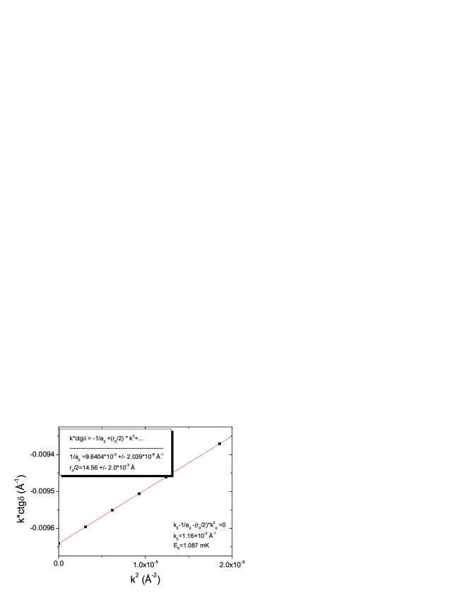
Figure 5: ”(Color online)” Extrapolation of He tetramer excited state binding energy from the He-He₃ scattering calculations. Low energy phase shift fit is made for k*ctg$\delta$ values as a linear function of momentum squared (k²).

It follows from Eq. (26) that in order to obtain the unknown binding energy it is sufficient to know the low energy coefficients $a_{0}$ and $r_{0}$. The scattering length value $a_{0}$ has been already determined and the effective range $r_{0}$ can be extracted by fitting with Eq. (25) the He-He₃ low energies phase shifts. The corresponding extrapolation procedure is illustrated in Fig. 5. One can see that inside the considered momentum region, close to $k=|k_{0}|$, the effective range expansion works perfectly well. The obtained binding energy, $\Delta B_{0}=1.087mK$, should not suffer much from higher order momentum terms in the expansion (25). Nevertheless, the He-He₃ effective range is pretty large $r_{0}$=29.1 $\AA$ and influences significantly the extrapolated binding energy value. By ignoring this term, one would get

$$\Delta B^{(0)}_{0}=\frac{\hbar^{2}}{2\mu_{3+1}a_{0}^{2}},$$ (27)

and a binding energy of only $\Delta B^{(0)}_{0}=0.751mK$ will be obtained, i.e. a value by 30% smaller.

We finally predict the existence of a $L^{\Pi}=0^{+}$ tetramer excited state with binding energy $B^{*}_{He_{4}}=\Delta B_{0}+B_{He_{3}}=127.5$ mK. This value compares well with the EFT prediction Platter discussed above, which gives the range $B^{*}_{He_{4}}\in[128-130]$ mK, a dispersion due to the fact that the interpolation was done for the total binding energy and not the sensibly smaller relative value $\Delta B_{0}$.

The validity of the procedure we use to obtain the binding energy of the excited tetramer can be verified in the dimer case, for which direct bound state calculations causes no difficulty. The procedure is illustrated in Fig. 6. The accurate dimer binding energy is $B_{He_{2}}=1.30348$ mK, a value very close to $\Delta B_{0}=1.087$ mK, and allows to control the inaccuracy made when disregarding higher order terms in expansion (25). By considering only two terms in the expansion (25) we have got $B_{He_{2}}=1.3036$ mK, only differing in the fifth significant digit from the directly calculated value. In addition, the He-He potential effective range extracted by fitting the low energy phase shift is $r_{0}$=7.337 $\AA$. This value can be independently calculated applying the Wigner formulae from zero-energy scattering wave function, which gives $r_{0}$=7.326 $\AA$, in nice agreement with the extrapolated one. Such an agreement demonstrates the validity of our approach.

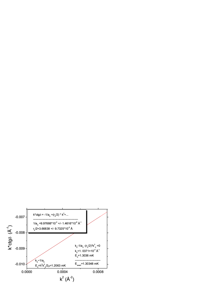
Figure 6: ”(Color online)” He dimer binding energy extrapolated from He-He scattering calculations. Low energy phase shift k*ctg$\delta$ is fitted with a linear function of $k^{2}$. Exact k*ctg$\delta$(k²) values are indistinguishable from the linear fit.

One should however mention that the very same procedure is not applicable to the trimer excited state calculation. If done, it would lead to a complex momentum $k_{0}=(1.3\pm 0.8i)\cdot 10^{-2}$ $\AA^{-1}$. This is a consequence of a dimer binding energy almost as small as $\Delta B^{*}_{He_{3}}=B^{*}_{He_{3}}-B_{He_{2}}$. In this case, the scattering phase shifts are affected by two open thresholds and thus a single channel S-matrix theory is not appropriate. In He-He₃ scattering, the nearest threshold He₂-He₂ opens only for scattering energies E${}_{cm}\approx$124 mK and thus is well separated from the energy region of interest ($\sim$ 1 mK).

It is interesting to compare the effective ranges for He-He, He-He₂ and He-He₃ systems. They are respectively $r_{0}$=7.33, 79.0 and 29.1 $\AA$. It is not surprising that the atom-dimer effective range is the largest one: this is a consequence of a dimer ground state which is the most extended of the three considered targets. The atom-trimer effective range is more than a third of the atom-dimer one and is significantly larger than the range of the He-He potential. This suggest that the trimer ground state has a structure with a sizeable probability to find a single He atoms separated by 20-30 $\AA$ apart from its center.

We can still use the He-He₃ scattering w.f. to obtain a relatively good description of the tetramer excited state. In fact, the left hand side of FY equations 2 for the bound and zero-energy He-He₃ state differ only by a small energy term, which has a little effect on the w.f. inside the interaction region, dominated by large kinetic and potential terms. These functions sensibly differ only in the He-He₃ asymptotes, where they can be described analytically Merkuriev ; Yak_Merk_assympt as a tensor product of a strongly bound trimer in its ground state and a plane wave of the remaining He atom with energy E-E${}_{He_{3}}$. In practice, the two w.f. differ only by FY amplitudes contributing to the open channels. For zero-energy scattering, one has a linearly diverging open channel FY amplitude as described in Eq. (23). For bound state these amplitudes converge very slowly with a small exponential factor:

$$\mathcal{F}_{\alpha_{a}}^{K}(x,y,z)\sim\phi_{He_{3}}(x,y)e^{-\sqrt{\frac{2}{3}}k_{0}*z}$$ (28)

The closed channel FY amplitudes rapidly vanish being shrunken by a relatively large $e^{-\sqrt{\frac{m*B_{He_{3}}}{\hbar^{2}}}*\rho}$ exponent, with $\rho=\sqrt{x^{2}+y^{2}+z^{2}}$.

Using this approximation for the tetramer excited state wave function, we have calculated some of its properties, which are summarized in Table 2.

V Tetramer and trimer rotational states

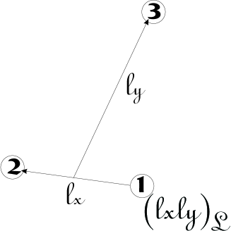
Figure 7: Coupling scheme for three-particle FY component.

Considering that ⁴He is a spinless atom, the rotational states of ⁴He-multimers can be classified according to their parity ($\Pi$) and total orbital angular momentum ($L$). FY components are very useful to classify these states as well as to analyse their properties. As we have mentioned in section II, the $l_{x}$ quantum number must be even (see Fig. 7). It follows that for He trimer, the $L^{\Pi}=0^{-}$ states are forbidden. Further we classify the He trimer states into those which can break into dimer and a freely propagating He atom, and those in which dimer states are forbidden by symmetry requirements. In the first group, we have states with $L^{\Pi}=(1^{-},2^{+},3^{-},...)$. To be decay stable, these states should be more bound than dimer. The other group is formed by the $L^{\Pi}=(1^{+},2^{-},3^{+},...)$ states, which can only break into three helium atoms.

Clearly, the $1^{-}$ is the most promising candidate for a trimer stable rotational state. This state is realized with the smallest partial angular momentum, i.e. $l_{x}+l_{y}\geq 1$, and consequently contains the smaller centrifugal terms in the Hamiltonian. The non-existence of this state would imply the non-existence of other states of the same decay group – i.e. $L^{\Pi}=(1^{-},2^{+},3^{-},...$) – since they involve larger centrifugal energies: $l_{x}+l_{y}\geq 2$. The existence of stable trimers in the second group is very doubtful; the most favorable would be the $2^{-}$ one, for which one has already $l_{x}+l_{y}\geq 3$.

In a similar way, we can classify the rotational states of He tetramer (see Fig. 1). In the first group, we have states $L^{\Pi}=(1^{-},2^{+},3^{-},..)$ for which the first decay threshold is the trimer ground state. The most promising state inside this group is the $1^{-}$ one. For this state, the condition $l_{x}+l_{y}+l_{z}\geq 1$ must be satisfied.

In the second group, we have trimer decay stable states $L^{\Pi}=(1^{+},2^{-},3^{+},..).$ These states can neither break into trimer-atom pair nor into two dimers: their reference threshold is dimer plus two free atoms. $L^{\Pi}=0^{-}$ state represents a special case: it can be broken only into four free atoms.

The FY formalism we are using allows to calculate multiparticle rotational states with the same ease as zero angular momentum ones. However, none of trimer or tetramer rotational states have been found stable. The non-existence of weakly bound states can be easily verified using low energy scattering techniques for trimer and tetramer states in the first decay groups (two cluster). In addition, the calculated scattering length turns out to be an indicator for the strength of the interaction between the scattered clusters and thus tests if nearthreshold bound or resonant states are present.

For atom-dimer scattering in 1^-, one obtains a large positive scattering length $(a_{1})^{\frac{1}{3}}$=114.2 $\AA$. If He-He interaction is changed, this length scales with the dimer size. If we add a small attractive three-body interaction to force a trimer binding without affecting dimer, this scattering length becomes smaller. In fact, when the attractive three-body force is weak, this scattering length reduces very slowly. Only when this additional force becomes rather strong, close to the critical value binding 1^- trimer, the scattering length falls down to -$\infty$. It crosses a singularity, passing from -$\infty$ to +$\infty$ at the value where 1^- trimer bound state appears, and then again stabilizes to large positive value. This clearly indicates that no trimer rotational state exist with quantum numbers $L^{\Pi}=(1^{-},2^{+},3^{-}...)$. An even much stronger attractive three-body force is required to bind the second group $L^{\Pi}=(1^{+},2^{-},3^{+},...)$ states, thus excluding the possible existence of bound or even nearthreshold resonant He trimer states.

The case of rotational tetramers is identical to the trimers one. A positive scattering length $(a_{1})^{\frac{1}{3}}\approx$12.28 $\AA$ is also obtained for He-He₃ scattering with $L^{\Pi}=1^{-}$. This value is sensibly smaller than the one for $1^{-}$ atom-dimer scattering, which simply results from the scaling with the target size. As in trimers case, one has to apply a strong additional attractive force to reduce this scattering length to -$\infty$, i.e. to force the $1^{-}$ tetramers binding. Tetramers in the second decay group, as well as $L^{\Pi}=0^{-}$, seem to be even less favorable: they require an even stronger additional force to be bound. We conclude therefore that no bound or even nearthreshold resonant states should exist for tetramers with $L^{\Pi}\neq 0^{+}$.

VI Summary

In this paper, we have outlined Faddeev-Yakubovski equation formalism in configuration space. It enables a consistent description of bound and scattering states in multiparticle systems. This formalism was applied to study the lightest ($N=2,3,4$) systems of He atoms using realistic He-He interaction. We have presented accurate calculations for bound He trimer and tetramer states, as well as for low energy atom-dimer and atom-trimer scattering.

Our main results concern the He tetramer states. We have obtained a tetramer ground state binding energy of $B=558$ mK, in perfect agreement with the most accurate variational results.

The first realistic calculation of He-He₃ scattering length has been achieved, with the prediction $a_{0}$=104 $\AA$. Such a large value indicates the existence of a tetramer excited state close to the trimer ground state threshold.

Its binding energy can hardly be determined in a direct bound state calculation, due to the difficulties in accommodating a very extended wave function. We have shown that this energy can be obtained by applying an effective range expansion to low energy 1+3 scattering states. We predict the existence of a $L^{\Pi}=0^{+}$ He tetramer excited state with a binding energy of 127.5 mK, situated 1.09 mK below the trimer ground state.

Finally, we have studied the possible existence of rotational states in three and four atomic He compounds. It has been shown that neither the He trimer nor the tetramer have bound rotational ($L^{\Pi}\neq 0^{+}$) states. The existence of corresponding nearthreshold resonances is also doubtful.

Acknowledgements: Numerical calculations were performed at Institut du Développement et des Ressources en Informatique Scientifique (IDRIS) from CNRS and at Centre de Calcul Recherche et Technologie (CCRT) from CEA Bruyères le Châtel. We are grateful to the staff members of these two organizations for their kind hospitality and useful advices.

References

- (1) S. Datz, G. W. F. Drake, T. F. Gallagher, H. Kleinpoppen, and G. zu Putlitz: Rev. Mod. Phys. 71 (1999) S223.
- (2) F. Luo, G.C. McBane, G. Kim, C.F. Giese and W.R. Gentry: J. Chem. Phys. 98 (1993) 3564.
- (3) W. Schollkopf and J.P. Toennies: Science 266 (1994) 1345.
- (4) R.A. Aziz, M. J. Slaman: J. Chem. Phys 94 (1991) 12:8047.
- (5) A. R. Janzen and R. A. Aziz: J. Chem. Phys. 103 (1995) 9626.
- (6) R. A. Aziz, F. R. W. McCourt and C. C. K. Wong: Molecular Physics 61 (1987) 1487.
- (7) R. A. Aziz and M. J. Slaman: J. Chem. Phys. 94 (1991) 8047.
- (8) K. T. Tang, J. P. Toennies and C. L. Yiu: Phys. Rev. Lett. 74 (1995) 1546.
- (9) A. R. Janzen and R. A. Aziz: J. Chem. Phys. 107 (1997) 914.
- (10) V. Efimov: Phys. Lett. B 33 (1970) 563; Nucl. Phys. A 210 (1973) 157.
- (11) D.B. Kaplan: arXiv:nucl-th/9506035
- (12) G.P. Lepage: arXiv:nucl-th/9706029.
- (13) E. Braaten, H.W. Hammer: cond-mat/0410417 and refferences therein.
- (14) L. Platter, H.W. Hammer and Ulf-G. Meißner: Phys. Rev. A 70 (2004) 052101
- (15) T. Cornelius and W. Glöckle: J. Chem. Phys. 85 (1986) 3906.
- (16) A.K. Motovilov, W. Sandhas, S.A. Sofianos and E.A. Kolganova: Eur. Phys. J. D 13 (2001) 33.
- (17) P. Barletta, A. Kievsky: Phys. Rev. A 64 (2001) 042514.
- (18) V. Roudnev: Chem. Phys. Lett. 367 (2003) 95 .
- (19) E. A. Kolganova, A. K. Motovilov, and W. Sandhas: Phys. Rev. A 70 (2004) 052711.
- (20) L.D. Faddeev: Zh. Eksp. Teor. Fiz. 39, (1960) 1459 [Sov. Phys. JETP 12, (1961) 1014].
- (21) O.A. Yakubowsky: Sov. J. Nucl. Phys. 5 (1967) 937.
- (22) S.P. Merkuriev and S.D. Yakovlev: Teor. Math. Phys. 56 (1983) 60.
- (23) S.P. Merkuriev, L.D. Faddeev: Quantum Scattering Theory for systems of several particles, Doderecht, Boston: Kluwer Academic Publishers (1993)
- (24) S.P. Merkuriev, A.K. Motovilov and S.D. Yakovlev: Teor. Math. Phys. 94 (1993) 435.
- (25) F. Ciesielski, Thèse Univ. J. Fourier (Grenoble) (1997).
- (26) R. Lazauskas: PhD Thesis, Université Joseph Fourier, Grenoble (2003); http://tel.ccsd.cnrs.fr/documents/archives0/00/00/41/78/.
- (27) J. Carbonell, C. Gignoux, and S. P. Merkuriev: Few-Body Syst. 15 (1993) 15.
- (28) E. Nielsen, D. V. Fedorov, and A. S. Jensen: J. Phys. B 31 (1998) 4085.
- (29) D. Blume and Chris.H. Greene: J. Chem. Phys. 112 (2000) 18:8053.
- (30) V. Roudnev and S. Yakovlev: Chem. Phys. Lett. 328 (2000) 97.
- (31) A. Kalinin, O. Kornilov, L. Rusin, J.P. Toennies and G.Vladimirov: Phys. Rev. Lett.93 (2004) 163402
- (32) T. Gonz’alez-Lezana, J. Rubayo-Soneira et al.: Phys. Rev. Lett. 82 (1999) 1648.
- (33) B.D. Esry, C.D. Lin, C.H. Greene, and D. Blume: Phys. Rev. Lett. 86 (2001) 4189.
- (34) B.D. Esry, C.D. Lin and C.H. Greene: Phys. Rev. A 54 (1996) 394.
- (35) E. Nielsen, D.V. Fedorov, A.S. Jensen: Phys.Rev.Lett.82 (1999) 2844.
- (36) E.A. Kolganova and A.K. Motovilov: Phys. Atom. Nucl.62, No.7 (1999), 1179 [arXiv: physics/9808027].
- (37) J. Carbonell and C. Gignoux: Few-Body Syst. Suppl. 7 (1994) 270.
- (38) S. Nakaichi, Y. Akaishi, H. Tanaka, T. K. Lim. Phys. Lett. A 68 (1978) 36.
- (39) D. Bressanini, M. Zavaglia, M. Mellab and G. Morosic: J. Chem. Phys.112 (2000) 2:717
- (40) M. Lewerenz: J. Chem. Phys. 106 (1997) 11:4596.
- (41) R. Guardiola, M. Portesi and J. Navarroa: Phys. Rvev. B 60 (1999) 6288.
- (42) S. Nakaichi, T. K. Lim, Y. Akaishi, and H. Tanaka: Phys. Rev. A 26, (1982) 32; S. Nakaichi-Maeda and T.K. Lim: Phys. Rev. A 28 (1983) 692.
- (43) I.N. Filikhin1, S.L. Yakovlev, V.A. Roudnev and B. Vlahovic: J. Phys. B 35 (2002) 501.
- (44) L.H. Thomas: Phys. Rev. 47 (1935) 903.
- (45) A.E.A. Amorim, T. Frederico and L. Tomio: Phys. Rev. C56 (1997) R2378.
- (46) E. Nielsen, D. V. Fedorov, A. S. Jensen, E. Garrido: Phys. Rep. 347 (2001) 373.
- (47) A.A. Kvitsinskii, Yu.A. Kuperin, S.P. Merkuriev: Sov. J. Part. Nucl. 17 (1986) 113.