Scale invariant distribution and multifractality of volatility multipliers in stock markets

Abstract

The statistical properties of the multipliers of the absolute returns are investigated using one-minute high-frequency data of financial time series. The multiplier distribution is found to be independent of the box size $s$ when $s$ is larger than some crossover scale, providing direct evidence of the existence of scale invariance in financial data. The multipliers with base $a=2$ are well approximated by a normal distribution and the most probable multiplier scales as a power law with respect to the base $a$. We unravel that the volatility multipliers possess multifractal nature which is independent of construction of the multipliers, that is, the values of $s$ and $a$.

,

1 Introduction

It has been a long history that physicists show interests on financial markets, which can be at least traced back to 1900 when Bachelier modeled stock prices with Brownian motions [1]. In the middle of last century, Mandelbrot proposed to characterize the tail distributions of income and cotton price fluctuations with the Pareto-Lévy law and applied R/S analysis to investigate the temporal correlations in the evolution of stock prices [2]. In recent years since the seminal work of Mantegna and Stanley [3], Econophysics has attracted extensive interest in the physics community.

As an analogue to turbulence, many time series observed in the financial markets are reported to possess multifractal properties [4, 5], such as the foreign exchange rate [4, 5, 6, 7, 8, 9, 10, 11], gold price [8], commodity price [12], stock price [12, 13, 14, 15, 16, 17], stock market index [18, 19, 20, 21, 22, 23, 24, 25, 26, 27, 28], to list a few. Extensive methods have been adopted to extract the empirical multifractal properties in financial data sets, for instance, the wavelet transform module maxima (WTMM) [29, 30, 31] and the multifractal detrended fluctuation analysis (MF-DFA) [32]. A time series of the price fluctuations possessing multifractal nature usually has either fat tails in the distribution or long-range temporal correlation or both [32]. However, possessing long memory is not sufficient for the precence of multifractality and one has to have a nonlinear process with long-memory in order to have multifractality [33]. In many cases, the null hypothesis that the reported multifractal nature is stemmed from the large fluctuations of prices can not be rejected [34].

Here, we propose to investigate the multifractal nature of absolute returns of stocks based on the multiplier method, again, borrowed from turbulence [35, 36, 37, 38]. Our goal is to provide direct evidence of scale invariance in the distribution of the multipliers. The concept of multiplier was originally introduced by Novikov to describe the intermittency and scale self-similarity in turbulent flows [39]. The scale-invariant multiplier distribution is argued to be more basic than the standard $f(\alpha)$ curve [35, 36]. In addition, it allows us to extract both positive and negative parts of the $f(\alpha)$ function with exponentially less computational time and is more accurate than conventional box-counting methods [35, 36].

2 Description of the data set

We adopt a nice high-frequency data set recording the S&P 500 index to ensure better statistics in our analysis. The record contains quoted prices $I(t)$ of the index, covering eighteen years from Jan. 1, 1982 to Dec. 31, 1999. The sampling interval is one minute. As usual, the nontrading time periods are treated as frozen such that we count merely the time during trading hours and remove closing hours, weekends, and holidays from the data. The size of the data set is about 1.7 million.

The return $r(t)$ over a time scale $\Delta t$ is defined as follows

$$r(t)=\ln[I(t)]-\ln[I(t-\Delta t)]~{},$$ (1)

whose absolute is a measure of the volatility. In this letter, the time scale is $\Delta t=1$ min. We can construct an additive measure in the time interval $[t_{1},t_{2}]$, which is the sum of absolute returns:

$$\mu([t_{1},t_{2}])=\sum_{t=t_{1}}^{t_{2}}|r(t)|~{}.$$ (2)

The quantity $\mu([t_{1},t_{2}])$ is actually a measure of the volatility on the time interval $[t_{1},t_{2}]$ [40]. The time series $|r(t)|$ is partitioned into boxes of identical size $s$. Each of these mother boxes is further divided into $a$ daughter boxes. The multiplier $m$ is determined by the ratio of the measure on a daughter box to that on her mother box [36]. Therefore, the multiplier is dependent of $a$ and $s$ and can be denoted as $m_{a,s}$ when necessary.

3 Scale invariant distribution

Figure 1(a) presents the probability densities $p_{a,s}(m)$ of the multiplier $m$ for four different box sizes $s=30$, $60$, $120$, and $180$ with the same base $a=2$. All curves are symmetric with respect to $m=0.5$ such that $p_{2,s}(m)=p_{2,s}(1-m)$ by definition and close to Gaussian. The solid lines are the best fits to normal distributions, whose fitted standard deviations are $\widehat{\sigma}=0.089$ for $s=30$, $\widehat{\sigma}=0.073$ for $s=60$, $\widehat{\sigma}=0.068$ for $s=120$, and $\widehat{\sigma}=0.069$ for $s=180$, respectively. The corresponding r.m.s. of the fit residuals are $0.050$, $0.068$, $0.050$, and $0.068$. Note that the mean $\mu=1/2$ is fixed in the fitting procedure. It is evident that $\widehat{\sigma}$ decreases in regard to $s$ and tends to a constant for large $s$. This phenomenon is further manifested by Fig. 1(b), which plots the sample standard deviation $\sigma$ of the multipliers as a function of the box size $s$ for different base $a$. The inset shows the loglog plots of $\sigma$ against $s$.

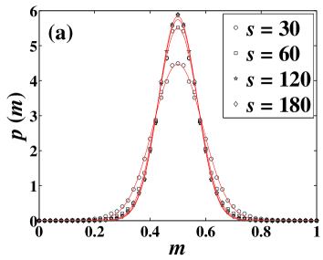
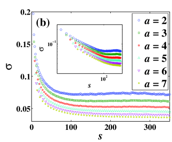
Figure 1: (color online). (a) Empirical probability density functions of the volatility multipliers with the base $a=2$ for different box sizes. The solid lines are fitted normal distributions. (b) Dependence of the sample standard deviation $\sigma$ as a function of $s$ for different bases. The inset shows the loglog plots of $\sigma$ against $s$.

One can see that there are two regimes in the $\sigma$ versus $s$ relation: $\sigma$ decays as a power law for small $s$ and saturates to a constant for large $s$. Roughly speaking, the crossover values of $s$ are the following: $s_{\times}\approx 80$ for $a=2$, $s_{\times}\approx 100$ for $a=3$, $s_{\times}\approx 120$ for $a=4$, $s_{\times}\approx 140$ for $a=5$, $s_{\times}\approx 150$ for $a=6$, and $s_{\times}\approx 150$ for $a=7$, respectively. In other words, the sample variance $\sigma^{2}$ in the case of $a=2$ has the fastest convergence rate to a constant.

Figure 2(a) shows the empirical probability density functions $p_{a,s}(m)$ of the multipliers for different bases $a=2$, $3$, and $5$ and different box sizes $s=150$, $210$, and $300$. For each $a$, $p_{a,s}(m)$ remains invariant in respect to $s$ when $s>s_{\times}$. In other words, there is a scaling range in which the volatility multiplier is scale invariant, whose distribution is independent of $s$. We shuffled the return series and found that the multiplier distributions are not scale invariant and the scaling range of $s$ disappears, as illustrated in Fig. 2(b). Therefore, $p_{a,s}(m)$ can be reduced to $p_{a}(m)$ in the scaling range. The shuffling test shows that long memory in the volatility plays an essential role in the appearance of scale invariance.

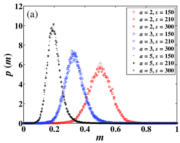
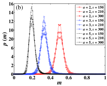
Figure 2: (color online). (a) Scale invariant distributions of volatility multiplier $m_{a,s}$ for different bases $a=2$, $3$, and $5$ and different box sizes $m=150$, $210$, and $300$. (b) Scale invariant distributions of volatility multiplier $m_{a,s}$ for the shuffled time series.

The most probable multipliers are also investigated in this work. For a given $s$, the most probable multiplier $m_{\max}$ with base $a$ is estimated such that $p_{a,s}(m_{\max})=\max[p_{a,s}(m)]$. Figure 3(a) presents the loglog plots of $m_{\max}$ versus $a$ for different values of $s$. One can observe that the data points for different $s$ collapse on a single line, showing a power-law dependence

$$m_{\max}\approx a^{-\beta}~{},$$ (3)

where $\beta=1.10\pm 0.02$ for $s=150$, $\beta=1.10\pm 0.01$ for $s=210$, and $\beta=1.09\pm 0.01$ for $s=300$, respectively. Intuitively, since a mother box is divided into $a$ daughter boxes, the sum of the $a$ multipliers is one and the multipliers is expected to aggregate around $1/a$. However, it is noteworthy that this power-law dependence is nontrivial, which does not hold in turbulence [36, 41, 42]. In Fig. 3(b) is shown $p_{a,s}(m_{\max})$ as a function of $s$ for different $a$. It is evident that $p(m_{\max})$ increases with $s$ and then approaches a plateau when $s>s_{\times}$. Figure 3 further verifies the scale-invariant nature of the volatility multiplier.

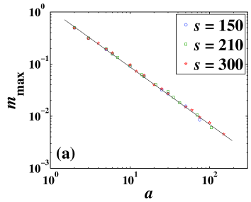
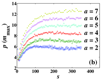
Figure 3: (color online). (a) Power law dependence of $m_{\max}$ versus $a$ for $s=150$, $210$, and $300$. (b) The saturation behavior of $p(m_{\max})$ in regards to $s$ for different $a$.

4 Multifractal analysis

It is shown that, for any two bases $a$ and $b$, the density functions are related through Mellin transform in the following form [36]

$$[\mathbb{M}\{p_{a}(m_{a})\}]^{1/\ln a}=[\mathbb{M}\{p_{b}(m_{b})\}]^{1/\ln b}~{},$$ (4)

where $\mathbb{M}$ stands for Mellin transform. Equivalently, we have

$$\frac{\ln\int_{0}^{1}m_{a}^{q}p_{a}(m_{a})dm_{a}}{\ln a}=\frac{\ln\int_{0}^{1}m_{b}^{q}p_{b}(m_{b})dm_{b}}{\ln b}~{}.$$ (5)

The scaling exponent $\tau(q)$ of the moment of $m_{a}$ can be obtained as follows [35, 36]

$$\tau(q)=-D_{0}-\frac{\ln\langle m_{a}^{q}\rangle}{\ln a}~{},$$ (6)

where $D_{0}$ is the fractal dimension of the support of the measure. In the current case, we have $D_{0}=1$. Note that the use of the Mellin transform may indeed appear natural in the framework of scaling and power-like functions, for instance, in the analysis of Weierstrass-type functions [43].

The local singularity exponent $\alpha$ and its spectrum $f(\alpha)$ are related to $\tau(q)$ through Legendre transforms: $\alpha(q)=\tau^{\prime}(q)$ and $f(\alpha)=q\alpha(q)-\tau(q)$. It follows that [35, 36, 44, 45, 46]

$$\alpha(q)=-\frac{\langle m_{a}^{q}\ln m_{a}\rangle}{\langle m_{a}^{q}\rangle\ln a}$$ (7)

and

$$f(\alpha)=\frac{\langle m_{a}^{q}\rangle\ln\langle m_{a}^{q}\rangle-\langle m_{a}^{q}\ln m_{a}^{q}\rangle}{\langle m_{a}^{q}\rangle\ln a}~{}.$$ (8)

Equations (5-8) predict that each of these characteristic multifractal arguments for fixed $q$ converges to constant in the scaling range and are independent of the base $a$ as well.

In order to test this prediction, we have to calculate first the scaling function $\tau(q)$ which requires that the integrand $m_{a}^{q}p_{a}(m_{a})$ converges for a given $q$ [47, 48]. We have investigated $m_{a}^{q}p_{a}(m_{a})$ for different values of $q$, $s$, and $a$. A typical dependence of $m_{a}^{q}p_{a}(m_{a})$ as a function of $m_{a}$ is shown in Fig. 4 for different values of $q$ with fixed box size $s=210$ and base $a=2$. The integrand diverges for large $m_{a}$ when $q$ is larger than 6. We shall nevertheless investigate scaling functions for $q\leqslant 8$ for comparison. Moreover, Fig. 4 indicates that the integrand diverges when $q\leqslant-1$ and the associated negative moments do not exist. This is a direct consequence of the fact that $p_{a}(0)\neq 0$. Indeed, there are time moments when the local returns are zero so that the probability density at $m_{a}=0$ is apart from zero, i.e., $p_{a}(0)\neq 0$. Approximately, for a small number $\delta$, $p(m)=p(0)$ is a constant for $m<\delta$. Posing $\int_{\delta}^{1}m^{q}p(m)dm=C$, we have $\int_{0}^{1}m^{q}p(m)dm=\int_{0}^{\delta}m^{q}p(m)dm+C=p(0)\frac{1}{q+1}m^{q+1}\left|\right._{0}^{\delta}+C$. Therefore, we have $q>-1$, which is quite analogous to the situation in turbulence [49].

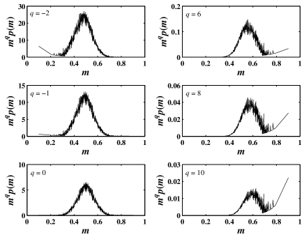
Figure 4: Numerical integrand $m^{q}p(m)$ as a function of $m$ for different values of $q$ with $s=210$ and $a=2$.

We now present in Fig. 5 the results of the multifractal analysis for $q$ varying from $-1$ to $8$. In Fig. 5(a) is shown the dependence of the scaling function $\tau(q)$ upon the box size $s$ for different values of $q$ and $a$. It is evident that, for large $s$, $\tau(q)$ is independent of $s$ for every $q$ under investigation. The $\tau(q)$ function reaches constant faster for small $a$. These results are in excellent agreement with the theoretical predictions. Figure 5(b) shows the dependence of the singularity spectrum $f(\alpha)$ on the box size $s$ for different values of $q$ and $a$. Again, we witness a range of scale invariance in which $f(\alpha)$ is independent of $s$. What needs to be emphasized is that, for $q=8$, the three $f(\alpha)$ curves with different $a$ do not converge due to bad statistics as shown by the left-middle panel of Fig. 4. We plot the three scaling functions $\tau(q)$ for $a=2$, $3$, and $5$ with respect to $q$ in Fig. 5(c). The error bars are estimated as the standard deviation over different $s$. Except for large $q$, the three $\tau(q)$ curves collapse on a single nonlinear curve. In addition, Fig. 5(d) shows the three singularity spectra $f(\alpha)$ in respect to the local singularity exponent $\alpha$ for the three bases. Again, the three curves collapse remarkably on a single curve when $q$ is not too large. Both Fig. 5(c) and Fig. 5(d) strongly indicate that the volatility multiplier possesses multifractal nature.

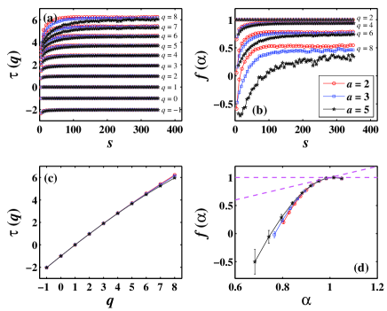
Figure 5: (color online). Multifractal analysis of absolute returns. (a) Dependence of $\tau(q)$ with respect to $s$ for different values of $q$ and different bases $a=2$, $3$, and $5$. (b) Dependence of $f(\alpha)$ with respect to $s$ for different values of $q$ and different bases $a=2$, $3$, and $5$. (c) Scaling function $\tau(q)$ obtained from Eq. (6) for different bases $a=2$, $3$, and $5$. (d) Singularity spectrum $f(\alpha)$ obtained from Eq. (7) and Eq. (8) for different bases $a=2$, $3$, and $5$.

An important feature of multifractals is the possible existence of negative dimensions in the multifractal spectrum, that is, $f(\alpha)<0$ for large or small $\alpha$ [50]. Negative dimensions are more common if the multiplier distribution is continuous [36, 44, 45, 46]. Figure 5(d) also shows that there are negative dimensions for large $q$ especially when $a$ is large. However, we should be cautious that the part of $f(\alpha)<0$ might be an artifact of bad statistics for large $q$ and $a$, as shown by the right panel of Fig. 4 and Fig. 5(b) as well. Since the multifractal functions are more reliable statistically for $a=2$, we argue that there is no negative dimension for $q\leqslant 8$. More data are required to investigate higher order moments and the issue of the existence of negative dimensions is still open.

In the development of Econophysics, the literature has witnessed increasing analogues between turbulence and finance. Multiplier analysis is a well-established method in the description of conservative quantities in turbulence [39, 35, 36, 37, 38]. Novikov predicted that the multiplier distribution $p(m)$ is independent of the scale $s$ as long as $s$ is well inside the inertial subrange [39]. Our finding provides further evidence of the analogue between turbulence and finance, except that the existence of negative dimensions that was reported in turbulence is not confirmed in our financial data. Moreover, the energy dissipation multiplier with $a=2$ follows approximately a triangular distribution, which is much flatter than the normal distribution of volatility multiplier in this work.

5 Conclusion

In summary, we have employed the multiplier method to investigate the volatility of high-frequency data of the S&P 500 index. The distribution of volatility multiplier is found to be independent of the time scale $s$ for different $a$ when $s$ is larger than some crossover scale $s_{\times}$. We unraveled that the volatility multipliers are scale invariant and have multifractal nature, which is independent of the construction of the multipliers (characterized by $s$ and $a$) in the scaling range.

Acknowledgments:

This work was partially supported by the National Natural Science Foundation of China (Grant No. 70501011) and the Fok Ying Tong Education Foundation (Grant No. 101086).

References

- [1] L. Bachelier, Théorie de la Spéculation, Ph.D. thesis, University of Paris, Paris (March 29 1900).
- [2] B. B. Mandelbrot, Fractals and Scaling in Finance, Springer, New York, 1997.
- [3] R. N. Mantegna, H. E. Stanley, Scaling behaviour in the dynamics of an economic index, Nature 376 (1995) 46–49.
- [4] S. Ghashghaie, W. Breymann, J. Peinke, P. Talkner, Y. Dodge, Turbulent cascades in foreign exchange markets, Nature 381 (1996) 767–770.
- [5] R. N. Mantegna, H. E. Stanley, Turbulence and financial markets, Nature 383 (1996) 587–588.
- [6] N. Vandewalle, M. Ausloos, Sparseness and roughness of foreign exchange rates, Int. J. Mod. Phys. C 9 (1998) 711–719.
- [7] F. Schmitt, D. Schertzer, S. Lovejoy, Multifractal analysis of foreign exchange data, Appl. Stoch. Models Data Analysis 15 (1999) 29–53.
- [8] K. Ivanova, M. Ausloos, Low -moment multifractal analysis of Gold price, Dow Jones Industrial Average and BGL-USD exchange rate, Eur. Phys. J. B 8 (1999) 665–669.
- [9] R. Baviera, M. Pasquini, M. Serva, D. Vergni, A. Vulpiani, Correlations and multi-affinity in high frequency financial datasets, Physica A 300 (2001) 551–557.
- [10] S. V. Muniandy, S. C. Lim, R. Murugan, Inhomogeneous scaling behaviors in Malaysian foreign currency exchange rates, Physica A 301 (2001) 407–428.
- [11] R. Xu, Z.-X. Gençay, Scaling, self-similarity and multifractality in FX markets, Physica A 323 (2003) 578–590.
- [12] K. Matia, Y. Ashkenazy, H. E. Stanley, Multifractal properties of price fluctuations of stock and commodities, Europhys. Lett. 61 (2003) 422–428.
- [13] A. Turiel, C. J. Pérez-Vicente, Multifractal geometry in stock market time series, Physica A 322 (2003) 629–649.
- [14] P. Oświȩcimka, J. Kwapień, S. Drożdż, R. Rak, Investigating multifractality of stock market fluctuations using wavelet and detrending fluctuation methods, Acta Physica Polonica B 36 (2005) 2447–2457.
- [15] L. Olsen, Multifractal geometry, Progress in Probability 46 (2000) 3–37.
- [16] A. Turiel, C. J. Pérez-Vicente, Role of multifractal sources in the analysis of stock market time series, Physica A 355 (2005) 475–496.
- [17] P. Norouzzadeh, G. R. Jafari, Application of multifractal measures to Tehran price index, Physica A 356 (2005) 609–627.
- [18] A. Bershadskii, Multifractal diffusion in NASDAQ, J. Phys. A 34 (2001) L127–130.
- [19] X. Sun, H.-P. Chen, Z.-Q. Wu, Y.-Z. Yuan, Multifractal analysis of Hang Seng index in Hong Kong stock market, Physica A 291 (2001) 553–562.
- [20] X. Sun, H.-P. Chen, Y.-Z. Yuan, Z.-Q. Wu, Predictability of multifractal analysis of Hang Seng stock index in Hong Kong, Physica A 301 (2001) 473–482.
- [21] I. Andreadis, A. Serletis, Evidence of a random multifractal turbulent structure in the Dow Jones Industrial Average, Chaos Solitons & Fractals 13 (2002) 1309–1315.
- [22] A. Z. Górski, S. Drożdż, J. Speth, Financial multifractality and its subtleties: An example of DAX, Physica A 316 (2002) 496–510.
- [23] M. Ausloos, K. Ivanova, Multifractal nature of stock exchange prices, Computer Physics Communications 147 (2002) 582–585.
- [24] M. Balcilar, Multifractality of the Istanbul and Moscow stock market returns, Emerging Markets Finance and Trade 39 (2) (2003) 5–46.
- [25] K. E. Lee, J. W. Lee, Multifractality of the KOSPI in Korean stock market, J. Korean Phys. Soc. 46 (2005) 726–729.
- [26] K. E. Lee, J. W. Lee, Origin of the multifractality of the Korean stock-market index, J. Korean Phys. Soc. 47 (2005) 185–188.
- [27] J. W. Lee, K. E. Lee, P. A. Pikvold, Multifractal behavior of the Korean stock-market index KOSPI, Physica A 364 (2006) 355–361.
- [28] Y. Wei, D.-S. Huang, Multifractal analysis of SSEC in Chinese stock market: A different empirical result from Heng Seng, Physica A 355 (2005) 497–508.
- [29] M. Holschneider, On the wavelet transformation of fractal objects, J. Stat. Phys. 50 (1988) 953–993.
- [30] J.-F. Muzy, E. Bacry, A. Arnéodo, Wavelets and multifractal formalism for singular signals: Application to turbulence data, Phys. Rev. Lett. 67 (1991) 3515–3518.
- [31] J.-F. Muzy, E. Bacry, A. Arnéodo, Multifractal formalism for fractal signals: The structure-function approach versus the wavelet-transform modulus-maxima method, Phys. Rev. E 47 (1993) 875–884.
- [32] J. W. Kantelhardt, S. A. Zschiegner, E. Koscielny-Bunde, S. Havlin, A. Bunde, H. E. Stanley, Multifractal detrended fluctuation analysis of nonstationary time series, Physica A 316 (2002) 87–114.
- [33] A. Saichev, D. Sornette, Generic multifractality in exponentials of long memory processes, Phys. Rev. E 74 (2006) 011111.
- [34] T. Lux, Detecting multifractal properties in asset returns: The failure of the “scaling estimator”, Int. J. Mod. Phys. C 15 (2004) 481–491.
- [35] A. B. Chhabra, K. R. Sreenivasan, Negative dimensions: Theory, computation and experiment, Phys. Rev. A 43 (1991) 1114–1117.
- [36] A. B. Chhabra, K. R. Sreenivasan, Scale-invariant multiplier distribution in turbulence, Phys. Rev. Lett. 68 (1992) 2762–2765.
- [37] B. Jouault, P. Lipa, M. Greiner, Multiplier phenomenology in random multiplicative cascade processses, Phys. Rev. E 59 (1999) 2451–2454.
- [38] B. Jouault, M. Greiner, P. Lipa, Fix-point multiplier distributions in discrete turbulent cascade models, Physica D 136 (2000) 125–144.
- [39] E. A. Novikov, Intermittency and scale similarity in the structure of a turbulent flow, J. Appl. Math. Mech. 35 (1971) 231–241.
- [40] B. Bollen, B. Inder, Estimating daily volatility in financial markets utilizing intraday data, J. Emp. Fin. 9 (2002) 551–562.
- [41] J. Molenaar, J. Herweijer, W. van de Water, Negative dimensions of the turbulent dissipation field, Phys. Rev. E 52 (1995) 496–509.
- [42] R. Kluiving, R. A. Pasmanter, Stochastic selfsimilar branching and turbulence, Physica A 228 (1996) 273–294.
- [43] S. Gluzman, D. Sornette, Log-periodic route to fractal functions, Phys. Rev. E 65 (2002) 036142.
- [44] W.-X. Zhou, Z.-H. Yu, On the properties of random multiplicative measures with the multipliers exponentially distributed, Physica A 294 (2001) 273–282.
- [45] W.-X. Zhou, H.-F. Liu, Z.-H. Yu, Anormalous features arising from random multifractals, Fractals 9 (2001) 317–328.
- [46] W.-X. Zhou, Z.-H. Yu, Multifractality of drop breakup in the air-blast nozzle atomization process, Phys. Rev. E 63 (2001) 016302.
- [47] V. S. L’vov, E. Podivilov, A. Pomyalov, I. Procaccia, D. Vandembroucq, Improved shell model of turbulence, Phys. Rev. E 58 (1998) 1811–1822.
- [48] W.-X. Zhou, D. Sornette, W.-K. Yuan, Inverse statistics and multifractality of exit distances in 3D fully developed turbulence, Physica D 214 (2006) 55–62.
- [49] B. R. Pearson, W. van de Water, Inverse structure functions, Phys. Rev. E 71 (2005) 036303.
- [50] B. B. Mandelbrot, Negative fractal dimensions and multifractals, Physica A 163 (1990) 306–315.