[Fortieth Hawaii International Conference on System Sciences, January 3-6, 2007, Big Island, Hawaii]
Stochastic Model for Power Grid Dynamics

Abstract

We introduce a stochastic model that describes the quasi-static dynamics of an electric transmission network under perturbations introduced by random load fluctuations, random removing of system components from service, random repair times for the failed components, and random response times to implement optimal system corrections for removing line overloads in a damaged or stressed transmission network. We use a linear approximation to the network flow equations and apply linear programming techniques that optimize the dispatching of generators and loads in order to eliminate the network overloads associated with a damaged system. We also provide a simple model for the operator’s response to various contingency events that is not always optimal due to either failure of the state estimation system or due to the incorrect subjective assessment of the severity associated with these events. This further allows us to use a game theoretic framework for casting the optimization of the operator’s response into the choice of the optimal strategy which minimizes the operating cost. We use a simple strategy space which is the degree of tolerance to line overloads and which is an automatic control (optimization) parameter that can be adjusted to trade off automatic load shed without propagating cascades versus reduced load shed and an increased risk of propagating cascades. The tolerance parameter is chosen to describes a smooth transition from a risk averse to a risk taken strategy. We present numerical results comparing the responses of two power grid systems to optimization approaches with different factors of risk and select the best blackout controlling parameter.

PACS: 89.75.-k, 05.10.-a, 02.50.-r

I Introduction

It is well-known that power grids are among the largest and most complex technological systems ever developed. These systems suffer periodic disturbances at various scales and some times these disturbances are so large to affect a considerable fraction of the power grid and induce considerable economic and social costs. For this reason, the vulnerability of power grids and more generally of interconnected transportation and communication networks has been recently studied extensively. In order to understand the global dynamics of power system blackouts a computationally efficient global system analysis approach is required in order to capture the overall response of the system to such events [4, 11]. Moreover, because this approach should be able to describe the random sequences of rare events that trigger large blackouts, it should have a stochastic character. On the other hand, any probabilistic risk assessment requires a large number of long simulations in order to determine the thought after risk indexes. Unfortunately, because the probability of these events is very low, it is very difficult to model the full complexity of the network’s dynamics over the very long time scales that are necessary for describing these rare events. One way to approach this difficult problem is to include simple, but representative, models for each component of this large and complex system as required in order to understand the global dynamics of power system blackouts. This is the approach followed by Dobson and coworkers [10, 4, 2, 3], who introduced a model that does not attempt to simulate the complex details of each blackout event, which may be comprised of complicated processes involving protection systems, dynamics, and human factors. Instead, the blackout cascades in this model are essentially instantaneous events due to dynamical redistribution of power flows and are triggered by probabilistic failures of overloaded lines. The size of blackouts is determined by solving a standard LP optimization of the generation dispatch, consistent with the power flow equations and operational constraints, and the redistribution of power flows is calculated using a linear load flow approximation.

Thorp and his collaborators  [31, 1, 8] perform a reliability study of transmission system protection devices using linear load flow approximation and linear programing optimization of generation dispatch and load shedding operations. Their approach uses a probabilistic model to simulate the incorrect tripping (sympathetic tripping) of lines and generators due to hidden failures of line or generator protection systems. The distribution of power system blackout size is obtained using importance sampling and blackout risk assessment and mitigation methods are also studied.

In another model, Rios et. al.  [26] propose a probabilistic cost/benefit analysis and calculate the expected blackout cost, which they equate with the value of grid security, using Monte Carlo simulations of a power system model that represents the effects of cascading line overloads, hidden failures of the protection system, and power system dynamic instabilities. In this approach the authors replace the complex time-dependent modeling of transient instability with a sophisticated probabilistic modeling using off-line computation of conditional probabilities based on the fault type and its location with respect to the vulnerability region of each generator.

Another example of advanced analysis of cascading failures and high-consequence contingencies, performed using TRELSS software, is described by Hardiman et. al. [14]. In its simulation approach mode, TRELSS simulates system vulnerability to cascading failures which are initiated by outages of lines, transformers, and generators due to overloads and voltage violations. The nodal voltages are monitored and if any load bus voltage magnitude becomes less than a specified “voltage collapse” threshold, the corresponding load is dropped. Similarly, voltages are controlled at generator buses as well and if they become less than a specified threshold, the corresponding generators are also tripped. Note though, the different conceptual approach to estimating voltage dependent effects, compared to the probabilistic approach of Rios et. al.  [26].

Ni et. al. [22] provide on-line risk-based security assessment (OL-RBSA) for rapid quantification of the security level associated with an existing or forecasted operating condition. Their probabilistic approach condenses contingency likelihood and severity functions into indexes that reflect probability risks. These indexes include overload security (flow violations and cascading overloads) and voltage security (voltage magnitude violations and voltage instability), while the risk assessment involves both the modeling of uncertainty as well as the modeling of severity functions assuming no operator’s action (such as redispatch) occurs. The goal is to reflect the consequence of the contingency and loading conditions, rather than the consequences of an operator’s decision.

These studies emphasize the importance of building representative stochastic models for the global system analysis of network reliability and of cascading failure risk. It is surprising that in most previous works, the modeling of the operator’s response to these complex and often unpredictable contingencies is very simple and, paradoxically, predictable. Because it is difficult to manage the technical difficulties associated with low-probability, high-impact events, modeling the often imperfect operator’s response should be an important component of the network reliability and blackout risk assessment. To emphasize this fact, we point out that the systematic control of large power systems in response to major contingency events is effectively nonexistent. The methods used are expert-based and are by rule not automated. Therefore, the inclusion of a human decision maker is critical [17]. Moreover, because most models generate only abstract blackouts, as sequences of technical failures propagating in space but instantaneous in time, they lack a faithful representation of the evolution of these events in time. This is unfortunate because it prevents us from using the sequence of system fluctuations, produced during the often slow, initiating phase that precedes large cascading events, to perform sophisticated pattern analyses aimed at predicting a developing blackout event as an anomaly detection problem.

Here we describe our first steps into the implementation of a power grid dynamic model that incorporates simple stochastic rules for the reliability of each grid component and offers a better description of line outages and line restoration events using a simple time-dependent approach. Unlike previous models, this model describes the utility response to various disturbances in an attempt to include a description of the human response to contingency events that is not always optimal due to either failure of the state estimation system or due to the incorrect subjective assessment of the severity associated with these events. In particular, this model is expected to serve as a general framework for a realist system-level analysis of the power grid from the viewpoint of the theory of complex networks [18, 29, 7, 20, 19, 12, 16, 32].

II Stochastic Grid Model

Our approach, inspired by the model introduced in [10, 4, 2, 3], computes the distribution of power flows using a linear load flow approximation, includes optimal generator dispatch and load shedding operations in order to alleviate operating contingencies, and models blackouts by overloads and outages of transmission lines. Disturbances in the grid are introduced by line outages due to unforeseen stochastic events. In order to describe the evolution of cascading events in their slow initiating stages, transmission lines failures in our model are due to line overheating due to excessive power flows. To describe this effect we monitor the evolution of the line temperature, and its slow dependence on flow redistributions, using as a model the conduction of heat in rods of small cross-section in which an electric current of constant strength is flowing. Further contributing to the slow evolution of cascades, is a line restoration model which prevents a damaged line from being put back in service before a random restoration time has passed. The model also has the ability to follow daily and seasonal changes in demand, although these features have not been used in the simple optimization experiments presented in this paper. We also provide a bounded rationality model for the operator’s response that is some times suboptimal due to either failure of the data acquisition equipment or due to the incorrect subjective assessment of the severity associated with cascading overloads. This further allows us to use a game theoretic framework for casting the operator’s response optimization into the choice of the optimal strategy which minimizes the operating cost. In the stochastic model introduced here the strategy space is defined by a line overload parameter which describes a smooth transition from a risk averse to a risk taken response.

The model and simulations were performed within the framework offered by the Power System Analyzer (PSA) [33], which is a suite of numerical tools developed at Los Alamos National Laboratory to permit model building, simulation, analysis, and graphical display of electric power transmission networks. Before presenting the details of the simulation algorithm we describe in detail each of the components of the stochastic model.

II-A Formulation of the DC power flow

We assume that the electrical transmission system operates in steady-state conditions and that this assumption holds even during the evolution of major disturbances in the system. This is obviously an approximation which is violated during the late stages of major disturbance events, but the model can be modified to better describe these events by modeling voltage-dependent phenomena.

In order to determine the steady-state operating conditions of the power grid, we should solve the full nonlinear power flow equations that provide information about the voltage magnitudes and phases and the active and reactive power flows along each transmission line. Unfortunately, since our simulations involve numerous power flow solutions for a power grid system that evolves in time under various random perturbations, solving repeatedly the full nonlinear power flow equations becomes computationally prohibitive. Moreover, we are interested in estimating the statistical properties of various quantities that characterize the system’s response to these perturbations, like the frequency distribution of blackout sizes, their duration, the distribution of inter-event times, etc., which also require the simulation of tens of thousands of blackout events. In addition, we are interested in estimating the optimal strategy necessary to mitigate the impact of blackout events. To address this problem, the full nonlinear equations pose very difficult nonlinear optimization problems. For all these reasons, we have chosen to linearize the power-flow equations and to solve instead the so called “DC” power flow equations that connect the flow of real power to the voltage phases of the system’s buses, which results in a completely linear, non-iterative power flow algorithm [34].

The DC power flow can only calculate real (MW) flows on transmission lines and gives no answers to what happens to voltage magnitudes or reactive (MVAR) flows. Assuming that all bus voltages phasors are 1.0 per unit in magnitude, and defining the matrix $\mathbf{B}$ by $B_{ij}=-b_{ij}$ if $i\neq j$ and $B_{ii}=\sum_{j\neq i}b_{ij}$, where $b_{ij}$ is the susceptance of the transmission line joining buses $i$ and $j$, the voltage phases $\theta_{i}$ are the solution of the linear power flow equation $\mathbf{P}=\mathbf{B}\mathbf{\Theta}$. Here, $\mathbf{P}$ is the vector whose $N-1$ components are the real powers injected at each node, except for a reference node (slack node) for which the injected real power is computed from the power balance between total generation and total load. The vector $\mathbf{\Theta}$ is the vector whose components are the voltage phases at each node in the network except the slack node which has phase zero. After solving the power flow equation for the vector $\mathbf{\Theta}$, the flow of real power along each transmission line is computed from $P_{ij}=b_{ij}(\theta_{i}-\theta_{j})$.

II-B Random line failure model

We assume that cascades in the grid are triggered by random line failure events and that lines fail independently of each other. For a line $l$, its random failure events are described by a Poisson process of constant rate $\lambda_{fl}$ such that the number of events in any interval of length $t$ follows a Poisson distribution with mean $\lambda_{fl}t$. Hence, the number of events which have occurred along line $l$ up to time $t$, $N_{l}(t)$, has the following probability distribution:

$$P_{l}\{N_{l}(t)=n\}=e^{-\lambda_{fl}t}\frac{(\lambda_{fl}t)^{n}}{n!}\,,\hskip 14.22636ptn\geq 0\,,$$ (1)

while its expectation is given by

$$E_{P_{l}}[N_{l}(t)]=\lambda_{fl}t\,,$$ (2)

which shows that $\lambda_{fl}$ is the average density of failure points. Assuming a constant reference rate per unit length, $\lambda_{f}$, for all lines in the network, the failure rate $\lambda_{fl}$ scales proportionally with the line length $L_{l}$ and is given by $\lambda_{fl}=\lambda_{f}L_{l}$.

In order to generate the random failure points $t_{n}$, $n=1,2,\ldots$, we sample from the stochastic process of rate $\lambda_{fl}$. The sampling process is very simple because the interval $x=t_{n}-t_{n-1}$ between two consecutive failure points has an exponential distribution of density [23],

$$f_{l}(x)=\lambda_{fl}e^{-\lambda_{fl}x}\,.$$ (3)

The first point in the sequence, $t_{1}$, is sampled using the fact that its random distance from the starting point of our simulation, $t_{0}$, is described by the same exponential distribution given by Eq. (3). Therefore, if $\xi_{0}$ is sampled from distribution (3) then $t_{1}=t_{0}+\xi_{0}$, and if $\xi_{1}$ is another number sampled from the same distribution then $t_{2}=t_{1}+\xi_{1}$, and so on. Sampling from an exponential distribution is numerically efficient, and is described in [25].

The failure rate used in our simulations, $\lambda=0.0001$, has not been benchmarked to utility experience. Our model assumes that failure events are independent in space and time but these are approximations that can be relaxed. For example, as we have already pointed out, hidden failures in the protection system can cause intact equipment to be unnecessarily removed from service (sympathetic tripping) following a fault on a neighboring component. Moreover, a component that failed yesterday is more likely to fail in a similar way the next day. One way to include these temporal correlations is to introduce a “hidden failure” (HF) state to each protection device and a Markov model describing the transition between the “ON”, “OFF” and “HF” states of the device as suggested in [24]. Similarly, weather effects (storms, hot weather, winds, etc) can induce correlated failures in space. These effects can be easily included in our model due to the dependence of the overloaded-line failure model on the ambient temperature and wind velocity. Depending on the weather conditions to which they are exposed, changes in the failure rates $\lambda_{fl}$ can also be introduced as described in  [26].

II-C Overloaded-line failure model

In order to model the failure of transmission lines due to loading over their transmission capacity, we consider the problem of conduction of heat in rods of small cross-section [6] in which an electric current of constant strength is flowing. We assume for simplicity that the transmission line is so thin that the temperature at all points of its cross-section is the same. We suppose that the transmission line has constant area of cross-section $\omega$, perimeter $p$, thermal conductivity $K$, electrical conductivity $\sigma$, density $\rho$, specific heat $c$, and diffusivity $\kappa$. We further assume that the heat flux across the surface of the line is proportional to the temperature difference between the surface and the surrounding medium and is given by $H(T-T_{0})$, where $T$ is the temperature of the line, $T_{0}$ is the temperature of the medium, and $H$ is the surface conductance. The problem of heat conduction then becomes one of linear heat flow in which the temperature is specified by the time $t$ and the position $x$ measured along the transmission line. Indeed, balancing the total rate of gain of heat in an element of volume bounded by the cross-sections at $x$ and $x+dx$ to the rate at which it gains heat across these faces minus the heat lost at the surface, we find the following heat equation,

$$\frac{\partial T(x,t)}{\partial t}=\kappa\frac{\partial^{2}T(x,t)}{\partial x^{2}}+\alpha I^{2}-\nu(T(x,t)-T_{0})\,,$$ (4)

where $\nu=Hp/(\rho c\omega)$, $\alpha=0.239/(\rho c\omega^{2}\sigma)$, $\kappa=K/(\rho c)$ and $I=P/V$ is the current in the line measured in amperes.

In order to estimate the surface conductance $H$ we will assume that the loss of heat across the surface of the line is due to forced convection. When fluid (gas or liquid) at temperature $T_{0}$ is forced rapidly past the surface of the line, it is found experimentally that the rate of loss of heat from the surface is given by $H(T-T_{0})$, with a value of the coefficient $H$ that depends on the velocity and the nature of the fluid and the shape of the surface [6]. For turbulent flow of air with velocity $u$ perpendicular to a circular cylinder of diameter $d$, $H=8\times 10^{-5}(u/d)^{1/2}$ $\textstyle{cal/(cm^{2}s\,K)}$.

Assuming that fluctuations in power flows along the transmission lines propagates much faster than any heat flow transients, and since the heat source is equally distributed along the line, we can neglect the spatial variation in temperature along the line in order to get a simple equation describing the time evolution in the temperature of the line in term of the power flowing through the line:

$$\frac{\partial T(x,t)}{\partial t}=\alpha I^{2}-\nu(T-T_{0})\,.$$ (5)

If the line is initially at temperature $T(0)$ and the power flowing through the line has the constant value $P$, the line temperature evolves according to this simple equation:

$$T(t)=e^{-\nu t}(T(0)-T_{e}(P))+T_{e}(P)\,,$$ (6)

where

$$T_{e}(P)=\frac{\alpha}{\nu}\frac{P^{2}}{V^{2}}+T_{0}\,$$ (7)

is the equilibrium temperature that the line will reach when $t\rightarrow\infty$. If at some moment the power flow changes, we reset the clock and the initial temperature and use the same equation to describe the evolution of line temperature starting from this moment on.

A transmission line failure due to excessive heating, followed by line sagging and tripping, will happen if the present power flow through the line exceeds the maximum line rating. For each line $l$, we denote by $T_{cl}$ the equilibrium temperature corresponding to a constant power flow equal to the line rating $P^{max}_{l}$, i. e.  $T_{cl}=T_{e}(P^{max}_{l})$. When the power flow through the line changes such that the new power flow $P_{l}$ exceeds $P^{max}_{l}$, the line will start heating toward the new equilibrium temperature. Since this equilibrium temperature exceeds $T_{cl}$, at some time $t_{cl}$ the line temperature will reach $T_{cl}$ and the line will fail. The failure time $t_{cl}$, measured from the moment when the grid topology and the line flow has changed, can be easily deduced from Eq. (6) and is given by

$$t_{cl}=\frac{1}{\nu}\ln\frac{T_{cl}-T_{e}(P_{l})}{T(0)-T_{e}(P_{l})}\,.$$ (8)

Let us further remark that the line rating, $P^{max}$, and some reference values for $u$ and $T_{0}$ are chosen to determine the critical temperature of the line. This means that on colder days, when $T^{\prime}_{0}<T_{0}$, the line will reach its critical, failure temperature, at a larger power flow $P^{\prime}>P^{max}$. Indeed, from the equation $T_{e}(P^{\prime})=T_{c}$ we get,

$$P^{\prime}=P^{max}\sqrt{1+(T_{0}-T_{0}^{\prime})\frac{\nu}{\alpha}\left(\frac{V}{P^{max}}\right)^{2}}\,.$$ (9)

Similarly, on a windier day, when $u^{\prime}>u$ and therefore $\nu^{\prime}>\nu$, the line fails when the power flow reaches a larger value $P^{\prime}$ given by

$$P^{\prime}=P^{max}\sqrt{\frac{\nu^{\prime}}{\nu}}\,.$$ (10)

It will be interesting to study how these weather effects, and the associated fluctuations in wind and temperature across a very large grid, will impact the risk of large blackout events. As we remarked before, these changes induce spatial correlation in the response of transmission lines to changes in power flows and, when overloaded, in the estimated failure times.

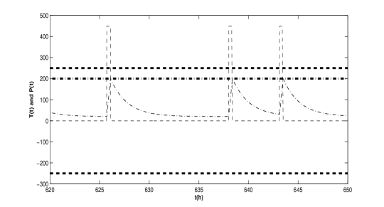
(a) Line I

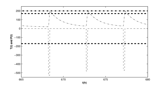
(b) Line II

Figure 1: The evolution of power flow (dashed line) and temperature (dash-dotted line) for two transmission lines in a simulation example. The time is measured in hours. The horizontal dash-dotted lines represents the critical temperatures at which each line failure due to overheating happens and the horizontal dashed lines represent the power line ratings. Both figures show the repeated failure of the lines shortly after a restoration event. Since the network has not fully recovered from the initial failures in other points of the network, each line restoration produces overflows which will shortly induce another overheating failure event. These examples were chosen to show that a suboptimal restoration strategy produces only temporary relief for a stressed system.

Finally, in order to keep the heat equation linear, we have omitted on the right hand side of Eq. (4) a cooling term that takes into account that each element of the surface of the rod loses heat by radiation to the surrounding medium — and provides cooling when the wind is absent. When this term is included, the right hand side of Eq. (5) acquires an additional cooling term $\frac{H^{\prime}p}{\rho c\omega}(T^{4}-T_{0}^{4})$, where $H^{\prime}$ is a constant. When the heating of the line is small and $T\approx T_{0}$, we can linearize this term and recover Eq. (5) with a corrected constant $\nu$ due to the fact that $H$ is now replaced with $H+4H^{\prime}$. When the heating of the line is large, we cannot make this approximation, the equation becomes nonlinear, and has to be integrated numerically. We have chosen not to do this, but we can easily include this effect at a reasonable computational cost.

Figure 1 shows a fragment from the evolution of the power flows and temperatures for two transmission lines during the evolution of a power grid subjected to random failure events. The dash-dotted lines represent the critical temperatures and the dashed lines the line ratings. The time segments were taken after increased line flows due to random component failures somewhere else in the network have induced the failure of each line due to overheating. Both figures show the repeated failure of the lines shortly after a restoration period. Since the network has not fully recovered from the initial failures, each line restoration produces overflows which will shortly induce another overheating failure event. In Figure 1 also we notice that due to thermal inertia effects the temperature evolution smoothes out the rapid power flow fluctuations.

II-D Line restoration model

We choose a very simple line restoration model that assumes that the restoration time $t_{r}$ has a constant component, $c$, plus a random variable $w$ that has an exponential distribution with parameter $\lambda_{r}$, i. e.

$$t_{r}=c+w\,,$$ (11)

where $w$ is sampled from the following exponential distribution:

$$f(w)=\lambda_{r}e^{-\lambda_{r}w}\,.$$ (12)

We further assume that $\lambda_{r}$ is the same for all lines in the system. The constant $c$ introduces a minimum restoration time that reflects the time to estimate which line was damaged and to ensemble and dispatch a restoration crew, before the restoration itself can take place. This model is not intended to be accurate, its parameters were not fit to any utility time-to-repair data, and was chosen for its simple parametrization. A more sophisticated estimated repair time, with a large number of parameters describing the type of component, its voltage, and environmental, temporal, and utility stress conditions is also an option implemented in our model, but which was not used for the present simulations. At the end of the restoration period for a damaged line the utility has a number of options for reconnecting the line to the power grid. These options are described in detail in the next subsection.

II-E Utility response model

One of the goals of this modeling approach is to describe the operator’s response to different contingencies, to estimate the optimal operator’s response, and to evaluate how a suboptimal response impacts the risk of large blackout events. The operator tries to minimize this risk by optimizing his response in a game against “nature” which performs random line failures or, more generally, random component failures, that can induce one or multiple line overloads. The random line (component) failure events are called type 3 events. When such an event happens, the operator has the option to respond with either deterministic or chance moves. For example, when a line overload is produced the operator has the option to either:

1. With probability $p_{1}$ shut down the line and protect it against failure and damage. We call this response a type 1 event.

2. With probability $p_{2}$, reflecting an erroneous estimation of the transmission line state, do nothing and let the line reach its critical temperature. We call this “response” a type 2 event.

3. With probability $p_{3}$ perform a partial generation dispatch and load shedding that can alleviate the overload.

Here the probabilities are such that $p_{1}+p_{2}+p_{3}=1$.

Unlike type 1 events, in which the line is not damaged, for type 2 events the line is damaged and a random restoration time necessary to fix the line must pass before it can be restored in service. The restoration event is called a type 0 event. When reconnecting lines, the operator first determines if there are islands in the system, which may be produced as lines are severed during the evolution of the event. If this is the case, it further determines if the reconnected lines join together two, or more, islands in the system. When this happens, we virtually restore the load demand to its initial value before the start of the reconnecting event. Here, the idea is that line restoration can fully recover the normal operating state of the system and, therefore, fully serve the loads. This reflects the fact that operator’s actions before the present restoration time might have shed loads in order to alleviate some overloaded lines observed in the system. It is also possible that, due to insufficient generation capacity, load shed was required by the constraint of power balance within an island.

After these virtual restorations and after solving for new power flows, the operator checks for the presence of overloaded lines. If there are no overloads, the line and load reconnection was successful and the operator proceeds with performing these operations by turning the virtual restorations into real events. If there are overloads the operator has a couple of options, for which we assign different probabilities ($p_{4}+p_{5}=1$):

1. with probability $p_{4}$, reconnects lines even though this process can induce overloads, of the lines themselves (most probably) or somewhere else in the system;

2. with probability $p_{5}$, performs another partial generation dispatch and load shedding that can alleviate the overload.

In order to implement the partial generation dispatch and load shed algorithm we have followed reference [2] and formulated the operator’s response as an optimization problem in which we solve the DC power flow equations while minimizing the following cost function:

$$C=\sum_{i\in\mathcal{G}}|P_{i}-P_{i0}|+W\sum_{j\in\mathcal{L}}(P_{j}-P_{j0})\,.$$ (13)

In this equation $P_{i0}$ and $P_{j0}$ are generator and load values, respectively, before turning on generator dispatch and load shed, while $P_{i}$ and $P_{j}$ are generator and load values after the overloads are removed. The cost function was chosen to minimize a trade-off between the change in generation (first summation over generator nodes $\mathcal{G}$) and the load shed (second summation over load nodes $\mathcal{L}$) necessary to eliminate the overloads. We assume that the cost of adjusting generators is the same and that loads share the same priority to be served. In order to force generator dispatch first, and simultaneously minimize the load shed in a contingency, we set a high price for load shed by choosing $W=100$ as in [2]. While restoring the loads after each contingency seems natural, generation restoration reflects the idea that the generation distribution is optimal from an economic view point and, for this reason, we would like to also restore the state of the generators. Even though the absolute value of the generation shift appears in the optimization problem, this optimization problem can be solved using linear programing techniques, following the method introduced in [10].

The minimization of the cost function is performed subject to the following constraints:

1. forcing an upper limit on the generator power: $0\leq P_{i}\leq P_{i}^{max},i\in\mathcal{G}$;

2. forcing the loads not to generate power: $P_{j0}\leq P_{j}\leq 0,j\in\mathcal{L}$;

3. forcing the power flow through the line within a $\alpha$ fraction of the line ratings: $-\alpha P_{l}^{max}\leq P_{l}\leq\alpha P_{l}^{max}$;

4. forcing the total power generated to exactly balance the total load demand: $\sum_{i\in\mathcal{G}\cup\mathcal{L}}P_{i}=0$.

We have introduced here a line overload parameter $\alpha$ which allows us to further represent either a risk averse response, when $\alpha<1$, or a risk taking response $\alpha>1$.

It is obvious that different choices for these probabilities can implement a large variety of operator’s actions. For example, by choosing $p_{3}=1$, we dispatch with probability one and we optimize the operator’s response by completely eliminating line overloading events, assuming that this is our goal. Because we can never eliminate the random line failure events, it is possible that this response will not guarantee a long term optimal response in reducing the average cost of cascading events. By always shedding loads to eliminate overloads, this response might produce numerous small cascades, whose added cost could be quite large. Therefore, it may be possible, as we discuss in Section V, to trade off the cost of small events versus an increased probability of generating larger, but less frequent, cascades, by not removing some line overloads.

III Simulation algorithm

The model is rich and complex in its possible behavior. In order to deal with the large variety of events we have time-ordered all events in an event list. There are a number of different event types that can be generated during the evolution of the system. The simulation begins by determining the time of the first type 3 event for each transmission line. The first type 3 event is initiating the event list. We have the possibility to introduce random load perturbations which happen on a time scale that is much smaller than the characteristic time scale for random failure events. After each new random load configuration we solve the power flow equations in order to determine the new state of the system. If these fluctuations introduce overloads, one of the utility response actions described in Section II is chosen according to its a priori probability.

When a failure event (type 3) is encountered, the line is damaged and a random restoration time $t_{r}$ is drawn from the probability distribution defined in the restoration model. A restoration event (type 0) for this line is introduced into the event list at time $t+t_{r}$ and a new random failure time for this failed line is generated. The next type 3 event is determined by finding the first type 3 event over all transmission lines and is introduced into the event list. To keep this list small, we always keep a single type 3 event in the event list, but the type 3 event times for all lines in the network are stored in a separate vector.

When an overloaded line is present in the system, there is a probability $p_{2}$ that the overloaded state of the line will be missed by the utility operator, due to an erroneous estimation of the state of the transmission line. As we know, this defines a type 2 event. In this case, there is a time delay, $t_{c}$, until the line reaches the critical temperature, that corresponds to its rating power, and fails. If the failure time $t+t_{c}$ happens before any other event in the event list, we include this event into the event list and remove any other events of type 1 or 2 that follow. Because this event damages the line, a random restoration time to fix the line must pass before it can be put back in service. Therefore, we also compute a restoration time $t_{r}$, sampled according to Eq. (11), and a restoration event corresponding to this line will be also included in the event list at time $t+t_{c}+t_{r}$. As we have just remarked, restoration events define type 0 events. The line can be restored only after time $t+t_{c}+t_{r}$, where $t$ is the present simulation time.

If $t+t_{c}$ comes after any other event, then we do not include this type 2 event in the event list, because a grid alteration will happen before it reaches its critical temperature. Indeed, earlier events may either modify its time of reaching the critical temperature, or may remove completely the overload and the line will cool down toward an equilibrium temperature below the critical temperature. For this reason, we also remove any other events of type 1 or 2 that follow an earlier type 2 event. We never remove type 3 and type 0 events from the event list.

Alternatively, with probability $p_{1}$, the operator shuts down the line in order to prevent its tripping due to overheating. As we have seen this defines a type 1 event. In this case, it is not necessary to repair the line, which can be set back in service according to the reconnection strategy described below at any time after the present time $t$.

No line can be reconnected until a restoration event happens because, as described in Section II, we assume that without a line reconnection the state of the system has not improved in order to prevent overloads in the reconnected lines or, possibly, somewhere else in the system.

After each restoration (type 0) event, we choose to reconnect all type 1 lines according to one of the reconnection strategies presented in detail in Section II. Sometimes reconnections result in overloads and, as a result, the utility may choose to remove the reconnected lines in order to remove these overloads and to restore the system to its old status before reconnections were attempted. In this case, each restoration event is written back into the event list as type 1 event and can be reconnected again at a later time when another reconnection events is encountered. For this reason, the event list will contain many type 1 events before the present simulation time $t$, for which reconnection attempts have failed.

Finally, at the beginning of a new event at event time $t$, the line temperatures are determined based on the known temperatures at the previous event (time step), $t-dt$, and the $dt$ time elapsed since the previous event. Thus, according to Eq. (6), we update the temperature of line $l$ to

$$T_{l}(t)=e^{-\nu dt}(T_{l}(t-dt)-T_{el}(P_{l}(t-dt)))+T_{el}(P_{l}(t-dt))\,.$$ (14)

Note that the power flow $P_{l}(t-dt)$ remains unchanged since the previous event time $t-dt$.

IV Sample Results for Cascading Failures

The first application of our time-event simulator is to look at overloaded-line cascading failures. This section illustrates a cascade simulation for a typical choice of the parameters of the model. In order to simulate this cascade event we only follow the evolution of real power flows and neglect the hourly load demand variations during the evolution of the event. Our goal is to compare the cost, in terms of load loss, of various mitigating responses in addressing the emerging system problems. The operator’s response ranges from choosing not to respond to eliminate overloads, to implement suboptimal generation dispatch, to respond with optimized system correction, i.e. generation dispatch and load shedding, to eliminate overloads. The critical algorithms of the cascade simulation include estimating restoration time of damaged components, estimating the time to disconnect for overloaded lines, recovering (when possible) load previously lost during contingency and islanding events, and attempting to reconnect previously disconnected lines.

Figure 2 shows the undamaged initial electrical power model. This transmission system consists of 100 nodes, 133 lines, 24 generators, and 5 interties (boundary conditions representing external networks not included within the transmission system). Small arrows indicate the direction of flow of the real power. The model features a high-voltage (230-kV) ring (light blue) that carries power to the lower voltage (138-kV, pink) and (69-kV, dark blue) lines that deliver power to the distribution network. The system is quite robust in that it generates more power than it uses, so it is a net exporter of power, and it does not depend upon external sources of power. About 2 GW of power are supplied to local customers.

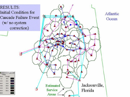
Figure 2: Undamaged initial electrical power model.

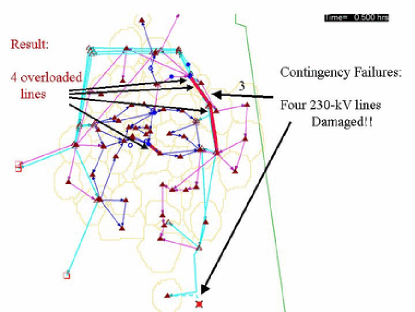
Figure 3: Starting contingency for electrical power model.

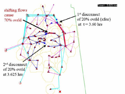
Figure 4: Two higher loaded lines are disconnected.

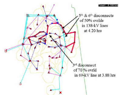
Figure 5: Three overloaded lines are disconnected.

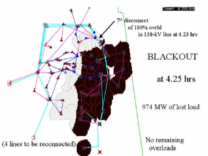
Figure 6: Estimated outage area.

Figure 3 shows the starting contingency where four 230-kV lines are damaged and lost from service. This contingency was chosen to sever the high capacity transmission paths between the largest generators in the northern section of the model from the southeast section of the model that has loads and no generation. This contingency creates four overloaded lines, two at about 120% loading and two at 108%. The two higher loaded lines are disconnected 3.6 hrs after the initial failures (see Figure 4). This shifts the power to create larger overload of 70% and 50% that are disconnected at 3.8 and 4.2 hrs (see Figure 5). This creates a situation where only one (overloaded) path remains to supply power to the southeast part of the model. This last line is disconnected (to protect it) at t = 4.23 hrs. This disconnection creates a black electrical island (i.e., no power can reach it). The estimated outage area is shown in Figure 6. The electrical company loses 974 MW of customer load at this time.

After the blackout begins, there are no overloads in the system. Also several of the previously disconnected lines are returned to service, but none of those lines connect the black island to the working island. It is not until hour 25.5, when the first one of the originally damaged 230-kV lines is replaced and restored to service, that the black island gets reconnected to the working network and all loads are recovered (with no overloads in the network). This ends the effect of the cascade event.

The result of this cascade example is summarized in Table I. In the discussion above, if the utility opts to do nothing after the initial four-line contingency, the relatively small overloads that result are eventually automatically disconnected to prevent them from being damaged, and the event cascades to cause a blackout affecting almost a GW of customer load. If, instead, the utility immediately sheds load after the initial event, all overloads are eliminated by shedding 108 MW. If one optimally sheds load and simultaneously adjusts the generation within the utility, then only 73 MW need be shed. The bottom line is that under the assumption of constant demand, choosing not to respond to eliminate overloads in the system can result in cascading failures where much larger loss of customer load can result. If we were also simulating the hourly variation in demand, the quantitative and possibly the qualitative conclusions could vary depending upon whether the initial contingency occurred during a period of demand growth or demand shrinkage. Such load-variation effects can be modeled using the new time-event simulator.

TABLE I: Results Summary of four 230-kV-Line contingency

Approach	Load Cost	Outage Duration	Effect
	(MW)	(hrs)
do nothing	974	21.3	cascade
			blackout
shed load	108	25.0	load shed
for overloads			waiting for repairs
shed load	73	25.0	load shed
and dispatch			waiting for repairs

V Optimal response

In this Section we discuss some of the features of the stochastic model when the utility response to line overloads is represented by the generation dispatch and load shed optimization algorithm. We choose to vary the line overload parameter $\alpha$ in order to describe a smooth transition from a risk averse $\alpha<1$ to a risk taken response for $\alpha>1$.

We want to test here two different optimization strategies against the response $\alpha=1$. The choice $\alpha=1$ defines the normal operating response represented by generation dispatch and load shedding to restore line flows at their critical value (line ratings). This should be compared to $\alpha<1$ case when the operator prevents the lines from even reaching their thermal ratings, or $\alpha>1$ when the operator decides to respond when the line flows reach a threshold higher than the line ratings. In the first case, $\alpha<1$, we trade off an increased load shed versus a smaller risk of generating large cascades. In the second case, $\alpha>1$, we trade off a smaller load shed versus an increased risk of generating large cascades. The question we ask is the following: Are there any model parameters for which one of this choices performs better than the optimization algorithm for $\alpha=1$? While we do not have as yet a complete answer to this question, we present here the results of our numerical experiments for the following model parameters: $\lambda_{f}$ = 0.0001, $c=3h$, $\lambda_{r}=0.2h^{-1}$ and $p_{3}=1$. We have run our experiments for the power grid model of 100 nodes, 24 generators, and 5 interties, that we have already introduced in Section IV. In order to compare the model responses for different $\alpha$ values we have estimated the cost of cascades per unit time, $C_{1}$, and the cost of cascades per event, $C_{2}$. The cost of a cascade, in MW hour, is defined as follows:

$$C=\int_{t_{s}}^{t_{e}}\Delta P(t)dT\,,$$ (15)

where $t_{s}$ is the time when cascade event starts, i. e.  the power served is less than the power demand, $t_{e}$ is the time when the cascade events ends with full service of the power demand, and $\Delta P(t)$ is the power shed at time $t$ during the cascade, $t_{s}\leq t\leq t_{e}$. In fact, the two cost functions we use can be defined as

$$C_{1} = \frac{\int_{t_{i}}^{t_{f}}\Delta P(t)dT}{t_{f}-t_{i}},$$ (16)

$$C_{2} = \frac{\int_{t_{i}}^{t_{f}}\Delta P(t)dT}{N}\,,$$ (17)

where $t_{i}$ is the starting time of the simulation, $t_{f}$ is the ending time of the simulation, while $N$ is the number of cascade events during the simulation time. Of course, $C_{2}$ is also the average cost of a cascade. Even though we call all events that shed power in the system “cascades”, not all events are cascading events in which a triggering failure produces a sequence of secondary failures that lead to blackout of a large area of the grid as presented in Section  IV. An exact characterization of the events, including their scaling properties will be presented elsewhere.

TABLE II: Comparison of utility responses with various optimization risk factors

$\alpha$	0.90	0.95	1.00	1.10	1.20	1.30	1.40
$C_{1}$	10.70	10.93	0.35	1.78	2.02	3.04	7.27
$C_{2}$	4026	4193	178	937	1032	1498	2966

The results of our numerical experiments are summarized in Table II. For the set of model parameters used in our experiments, the best response strategy is to implement the generation dispatch and load shed optimization with parameter $\alpha=1$, but we should remark that a global $\alpha$ parameter is probably not the most efficient implementation of this optimization idea. We expect that choosing a line dependent $\alpha$ value, that takes into account the importance of each line flow to the overall power transport in the system, could provide a more successful optimization strategy. For example, we can choose $\alpha=1$ for lines that carry the backbone of the power flow, and which will probably generate large flow redistributions for either $\alpha<1$ or $\alpha>1$, and a smaller or larger $\alpha$ value for the rest of the lines. A possible objection against this strategy can be the fact that the optimization approach proposed leads to damage to equipment, but it is useful to remember that August $14^{th}$, 2003 blackout cost billions of dollars in in economic losses but caused negligible equipment damage [27]. It is possible then that equipment damage that can significantly decrease the social cost of blackout events is a feasible prevention strategy. Moreover, one could conceivably extended this approach to other parameters or to other optimization strategies that can be used to assess vulnerabilities and to allocate protection devices and preventive maintenance responses, as described in [24]. The model can also be generalized to replace the unique power grid operator with a network of distributed, autonomous agents who share local information in order to coordinate their local responses to finding good global optimization solution as described in [15]. A decentralized approach may also benefit from the information provided by the structure of the underlying network of flows, as proposed in [20].

VI Conclusion

As more vulnerable networks emerge, due to the introduction of deregulated energy markets, the demand for a more reliable representation of the networks in order to correctly assess the operational security level of the transmission system will increase. At the same time, as the complexity of operating the grid grows, modeling the operator’s response to these challenging demands becomes increasingly critical and should match in sophistication the modeling of the grid itself. For these reasons, we have presented a model that attempts to provide a comprehensive representation of the complex behavior of both the grid dynamics under random perturbations and the operator’s response to the contingency events. This response is not always optimal due to either failure of the state estimation system or due to the incorrect subjective assessment of the severity associated with these events.

Furthermore, we have cast the optimization of the operator’s response into the choice of the optimal strategy for mitigating the impact of random component failure events and, possibly, for controlling blackouts. A first example was to test a generation dispatch and load shed algorithm for a range of risk factors that were trying to balance the risk of load shed versus the risk of generating large cascading events. This simple strategy space can be easily extended and we have suggested a few possible generalizations that are already the subject of intense research.

Moreover, the model can be used to test the conjecture that power grids operate close to a “critical” point as suggested by recent analysis of power system disturbance data [9, 5]. If this is confirmed, some aspects of the response of the system to random perturbations may have an universal character. In this case, the dynamics of the stochastic model for different parameters should exhibit the conjectured universal behavior. An analysis of this conjecture is the subject of our current research.

References

- [1] K. Bae and J. S. Thorp, “A stochastic study of hidden failures in power system protection”, Decision Support Systems, vol. 24, pp. 259-268, 1999.
- [2] B. A. Carreras, V. E. Lynch, I. Dobson, and D. E. Newman, “Critical Points and Transitions in an Electric Power Transmission Model for Cascading Failure Blackouts”, Chaos, vol. 12, no. 4, pp. 985-994, 2002.
- [3] B. A. Carreras, V. E. Lynch, I. Dobson, and D. E. Newman, “Complex Dynamics of Blackouts in Power Transmission Systems”, Chaos, vol. 14, no. 3, pp. 643-652, 2004.
- [4] B. A. Carreras, V. E. Lynch, M. L. Sachtjen, I. Dobson, and D. E. Newman, Modeling Blackout Dynamics in Power Transmission Networks, Hawaii International Conference on System Sciences, January 3-6, 2001, Maui, Hawaii.
- [5] B. A. Carreras, D. E. Newman, I. Dobson, and A. B. Poole, “Evidence for Self-Organized Criticality in a Time Series of Electric Power System Blackouts”, IEEE Transactions on Circuits and Systems I, vol. 51, no. 9, pp. 1733-1740, 2004.
- [6] H. S. Carslaw and J. C. Jaeger, Conduction of Heat in Solids, 2nd ed. Clarendon Press, Oxford, 1959.
- [7] D. P. Chassin and C. Posse, “Evaluating North American Electric Grid Reliability Using the Barabási-Albert Network Model”, Physica A, vol. 55, no. 2-4, pp. 667-677, 2005.
- [8] J. Chen and J. S. Thorp, A Reliability Study of Transmission System Protection via a Hidden Failure DC Load Flow Model, IEEE Fifth International Conference on Power System Management and Control, pp. 384-389, April 17-19, 2002.
- [9] J. Chen, J. S. Thorp, and M. Parashar, Analysis of Power System disturbance Data, Hawaii International Conference on System Sciences, January 3-6, 2001, Maui, Hawaii.
- [10] I. Dobson, B. A. Carreras, V. E. Lynch, and D. E. Newman, An Initial Model for Complex Dynamics in Electric Power System Blackouts, Hawaii International Conference on System Sciences, January 3-6, 2001, Maui, Hawaii.
- [11] I. Dobson, B. A. Carreras, V. E. Lynch, and D. E. Newman, Complex System Analysis of Series of Blackouts: Cascading Failure, Criticality, and Self-organization, Bulk Power Systems Dynamics and Control - VI, August 22-27, 2004, Cortina d’Ampezzo, Italy.
- [12] K. I. Goh, D. S. Lee, B. Kahng, and D. Kim, “Sandpile on Scale-Free Networks”, Physical Review Letters, vol. 91, no. 14, art. no. 148701, 2003.
- [13] J. J. Grainger and W. D. Stevenson, Jr. , Power System Analysis, 2nd ed. McGraw-Hill, New York, 1994.
- [14] R. C. Hardiman, M. Kumbale, and Y. V. Makarov, Multiscenario Cascading Failure Analysis Using TRELSS, Quality and Security of Electric Power Delivery Systems, CIGRE/IEEE PES International Symposium, pp. 176-180, October 8-10, 2003.
- [15] P. Hines, H. Liao, D. Jia, and S. Talukdar, Autonomous Agents and Cooperation for the Control of Cascading Failures in Electric Grids, Proceedings of the IEEE Conference on Networking, Sensing, and Control, March 2005, Tucson, Arizona.
- [16] P. Holme, and B. J. Kim, “Vertex Overload Breakdown in Evolving Networks”, Physical Review E, vol. 65, no. 6, art. no. 066109, 2002.
- [17] M. Ilic and P. Skantze, “Electric Power Systems Operation by Decision and Control”, IEEE Control Systems Magazine, vol. 20, no. 4, pp. 25-39, 2000.
- [18] R. Kinney, P. Crucitti, R. Albert, and V. Latora, “Modeling Cascading Failures in the North American Power Grid”, European Physical Journal B, vol. 46, no. 1, pp. 101-107, 2005.
- [19] Y. Moreno, R. Pastor-Satorras, A. Vazquez, and A. Vespignani, “Critical Load and Congestion Instabilities in Scale-Free Networks”, Europhysics Letters, vol. 62, no. 2, pp. 292-298, 2003.
- [20] A. E. Motter, “Cascade Control and Defense in Complex Networks”, Physical Review Letters, vol. 93, no. 9, art. no. 098701, 2004.
- [21] NERC (North American Electric Reliability council), 1996 system disturbances, (Available from NERC, Princeton Forrestal Village, 116-390 Village Boulevard, Princeton, New Jersey 08540-5731), 2002.
- [22] M. Ni,J. D. McCalley, V. Vittal, and T. Tayyib, “On-line Risk-Based Security Assessment”, IEEE Transactions on Power Systems, vol. 18, no. 1, pp. 258-265, 2003.
- [23] A. Papoulis, Probability, Random Variables, and Stochastic Processes, 2nd ed. McGraw-Hill, New York, 1984.
- [24] D. L. Pepyne, C. G. Panayiotou, C. G.Cassandras, and Y.-C. Ho, Vulnerability Assessment and Allocation of Protection Resources in Power Systems, Proceedings of the American Control Conference, June 25-27, 2001, Arlington, Virginia.
- [25] W. H. Press, S. A. Teukolsky, W. T. Vetterling, and B. P. Flannery, Numerical Recipes in C, 2nd ed. Cambridge University Press, 1992.
- [26] M. A. Rios, D. S. Kirschen, D. Jayaweera, D. P. Nedic, and R. N.Allan, “Value of Security: Modeling Time-Dependent Phenomena and Weather Conditions”, IEEE Transactions on Power Systems, vol. 17, no. 3, pp. 543-548, 2002.
- [27] U. S.-Canada Power System Outage Task Force, Final Report on the August 14th Blackout in the United States and Canada. United States Department of Energy and National Resources Canada, April 2004.
- [28] M. L. Sachtjen, B. A. Carreras, and V. E. Lynch, “Disturbances in Power Transmission System”, Physical Review E, vol. 61, no. 5, pp. 4877-4882, 2000.
- [29] A. Scire, I. Tuval, and V. M. Eguiluz, “Dynamic Modeling of the Electric Transportation Network”, Europhysics Letters, vol. 71, no. 2, pp. 318-324, 2005.
- [30] I. Steinwart, D. Hush, and C. Scovel, “A Classification Framework for Anomaly Detection”, Journal of Machine Learning Research, vol. 6, pp. 211-232, 2005.
- [31] J. S. Thorp, A. G. Phadke, S. H. Horowitz, and S. Tamronglak, “Anatomy of Power System Disturbances: Importance Sampling”, Electric Power and Energy Systems, vol. 20, no. 2, pp. 147-152, 1998.
- [32] D. J. Watts, “A Simple Model of Global Cascades on Random Networks”, Proceedings of the National Academy of Sciences U. S. A, vol. 99, no. 9, pp. 5766-5771, 2002.
- [33] K. A. Werley, The Power System Analyzer (PSA) Suite of Numerical Tools, Los Alamos National Laboratory report LA-UR-03-8268, pp. 1-61, July 2005.
- [34] A. J. Wood and B. F. Wollenberg, Power Generation, Operation, and Control, 2nd ed. John Wiley & Sons, New York, 1996.